Conditions for anti-Zeno-effect observation in free-space atomic radiative decay

Abstract

Frequent measurements can modify the decay of an unstable quantum state with respect to the free dynamics given by Fermi’s golden rule. In a landmark article [A. G. Kofman and G. Kurizki, Nature (London) $\mathbf{405}$, 546 (2000)], Kofman and Kurizki concluded that in quantum decay processes, acceleration of the decay by frequent measurements, called the quantum anti-Zeno effect (AZE), appears to be ubiquitous, while its counterpart, the quantum Zeno effect, is unattainable. However, up to now there have been no experimental observations of the AZE for atomic radiative decay (spontaneous emission) in free space. In this work, making use of analytical results available for hydrogen-like atoms, we find that in free space, only non-electric-dipolar transitions should present an observable AZE, revealing that this effect is consequently much less ubiquitous than first predicted. We then propose an experimental scheme for AZE observation, involving the electric quadrupole transition between $D_{5/2}$ and $S_{1/2}$ in the alkali-earth ions Ca⁺ and Sr⁺. The proposed protocol is based on the stimulated Raman adiabatic passage technique which acts like a dephasing quasi-measurement.

I Introduction

One of the more peculiar features of quantum mechanics is that the measurement process can modify the evolution of a quantum system. The archetypes of this phenomenon are the quantum Zeno effect (QZE) and the quantum anti-Zeno effect (AZE) Kofman and Kurizki (2000); Facchi et al. (2001). The QZE refers to the inhibition of the decay of an unstable quantum system due to frequent measurements Misra and Sudarshan (1977), and was observed experimentally for the first time with trapped ions Cook (1988); Itano et al. (1990) and more recently in cold neutral atoms Patil et al. (2015). The opposite effect, where the decay is accelerated by frequent measurements, was first called the AZE in Ref. Kaulakys and Gontis (1997), and was discovered theoretically for spontaneous emission in cavities Kofman and Kurizki (1996); Lewenstein and Rza̧żewski (2000), and first observed in a tunneling experiment with cold atoms (along with the QZE) Fischer et al. (2001), and recently with a single superconducting qubit coupled to a waveguide cavity Harrington et al. (2017). However, despite predictions that the AZE should be much more ubiquitous than the QZE in radiative decay processes Kofman and Kurizki (2000), it has never been observed to our knowledge for atomic radiative decay (spontaneous emission) in free space.

Here, we investigate the case of hydrogen-like atoms, for which the exact expression of the coupling between the atom and the free radiative field (cf. Moses (1973); Seke (1994)) allows us to derive an analytical expression for the measurement-modified decay rate. From this, we find that only non-electric-dipole transitions can exhibit the AZE in free space (i.e. non-dipole electric transitions and magnetic transitions of any multipolar order), which drastically limits the experimental possibilities to observe this effect. We start with a brief review of the general formal results about the measurement-modified decay rate in Sec. II, and we then apply, in Sec. III, this general framework to the case of electronic transitions in hydrogen-like atoms to derive an analytical expression of the measurement-modified decay rate in free space. Then, we discuss the experimental realizability of the described phenomenon in Sec. IV, and we identify a potential candidate: the electric quadrupole transition between $D_{5/2}$ and $S_{1/2}$ in Ca⁺ or Sr⁺. Conclusions are finally given in Sec. V.

II Monitored spontaneous emission: general analysis

We consider a two-level atom in free space, consisting of a ground state $\ket{\mathrm{g}}$ and an excited state $\ket{\mathrm{e}}$ separated by the Bohr energy $\hbar\omega_{0}$, and initially prepared in $\ket{\mathrm{e}}$. Due to the coupling with the modes of the electromagnetic (EM) reservoir, the atom will naturally decay to the ground state $\ket{\mathrm{g}}$, with a survival probability to stay in the excited state $\ket{\mathrm{e}}$ given by $P(t)=\text{exp}(-\Gamma t)$ (Wigner-Weisskopf decay Cohen-Tannoudji et al. (1989)). For the free dynamics (i.e. without measurements), the decay rate $\Gamma$ is given by the Fermi’s golden rule (FGR) Cohen-Tannoudji et al. (1989), and will be denoted by $\Gamma_{0}$ in the following.

In Ref. Kofman and Kurizki (2000), Kofman and Kurizki showed that frequent measurements on an excited two-level atom, i.e. repeated instantaneous projections onto the state $\ket{\mathrm{e}}$, lead to a broadening of its energy level, analogous to collisional broadening. Therefore, the atom probes a larger range of EM modes in the reservoir spectrum, and these new decay channels might modify the dynamics. Specifically, it was shown, within the rotating-wave approximation (RWA), that if frequent measurements are performed at short intervals $\tau$, the dynamics still follows an exponential decay, but with a measurement-modified decay rate given by Kofman and Kurizki (2000)

$$\Gamma=2\pi\int_{0}^{\infty}\mathrm{d}\omega\,F_{\tau}\left(\omega-\omega_{0}\right)R\left(\omega\right)\;.$$ (1)

The effects of the RWA on the QZE and AZE have been discussed in Refs. Zheng et al. (2008); Ai et al. (2010), showing no essential differences between the predictions made with and without the RWA in the case of the reservoir that we shall consider here. Moreover, for a discussion about a non-exponential decay, see Ref. Zhou et al. (2017).

In Eq. (1), the function $R(\omega)$ represents the reservoir coupling spectrum and is written

$$R(\omega)=\hbar^{-2}\sum_{k}|\bra{\mathrm{e},0}\hat{H}_{I}\ket{\mathrm{g},1_{k}}|^{2}\delta(\omega-\omega_{k})$$ (2)

where $\ket{\mathrm{g},1_{k}}=\ket{\mathrm{g}}\otimes\ket{1_{k}}$ is the outer product between the atomic state $\ket{\mathrm{g}}$ and the state of the EM field $\ket{1_{k}}$ containing one photon in the mode labelled by $k$, $\ket{\mathrm{e},0}=\ket{\mathrm{e}}\otimes\ket{0}$ is the outer product between the atomic state $\ket{\mathrm{e}}$ and the vacuum state of the EM field $\ket{0}$, and $\hat{H}_{I}$ is the interaction Hamiltonian. The function $F_{\tau}(\omega-\omega_{0})$, on the other hand, corresponds to the broadened spectral profile of the atom due to the frequent measurements at a rate $\nu=1/\tau$, and takes the form

$$F_{\tau}\left(\omega-\omega_{0}\right)=\frac{\tau}{2\pi}\text{sinc}^{2}\left((\omega-\omega_{0})\frac{\tau}{2}\right)$$ (3)

with $\text{sinc}(x)\equiv\text{sin}(x)/x$. Note that the spectral profile function can be generalized to the case where no assumption is made beforehand about the state that is being repeatedly prepared Chaudhry (2016). In Fig. 1 (a) (orange line), the function $F_{\tau}\left(\omega-\omega_{0}\right)$ is shown, centered on $\omega_{0}$ and with a width of about $2\pi\nu$. When $\nu\rightarrow 0$, $F_{\tau}\left(\omega-\omega_{0}\right)\rightarrow\delta\left(\omega-\omega_{0}\right)$ and Eq. (1) gives: $\Gamma\rightarrow 2\pi R(\omega_{0})$, which is the natural decay rate given by the FGR $\Gamma_{0}\equiv 2\pi R(\omega_{0})$, where only the single photon states of frequency $\omega_{0}$ contribute to the decay.

From Eq. (1), we can see that the measurement-modified decay rate corresponds to the overlap between the functions $R(\omega)$ and $F_{\tau}\left(\omega-\omega_{0}\right)$, and therefore depending on the profile of $R(\omega)$ in the interval around $\omega_{0}$, the system may experience an acceleration ($\Gamma>\Gamma_{0}$, AZE) or a deceleration ($\Gamma<\Gamma_{0}$, QZE) of the decay compared to the measurement-free decay. In the following, we aim at investigating the case of hydrogen-like atoms coupled to the free space EM field, for which the function $R(\omega)$ can be calculated analytically. This will allow us to highlight the conditions for an AZE observation in such systems. Before doing so, however, it is worth mentionning that in the perturbative treatment that we use, Eqs. (1) and (2) are valid to the first order (i.e. only one-photon processes are considered), and do not include higher-order contributions (i.e. two-photon and many-photon processes). For this approximation to be valid, we need to ensure that, compared to the spontaneous single-photon emission of the $\ket{\mathrm{e}}\rightarrow\ket{\mathrm{g}}$ transition considered, two-photon processes, which involve other atomic levels, are negligible. This can only be checked on a case-by-case basis for specific atoms. In Sec. IV, we consider the specific case of the electric quadrupole transition of Ca⁺, and we check that the single-photon emission is the dominant decay channel from the relevant excited state (in Sec. IV.1).

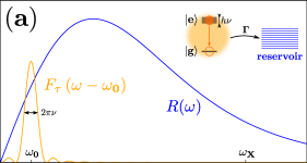
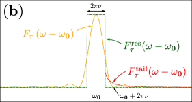
Figure 1: (a) Scheme of the broadened spectral profile $F_{\tau}(\omega-\omega_{0})$ (orange line) of an atom with transition frequency $\omega_{0}$ due to repeated measurements at a rate $\nu=1/\tau$ with $\tau$ the interval between each measurement, and reservoir coupling spectrum $R(\omega)$ (blue line) of the form of Eq. (6) with a cutoff frequency $\omega_{\mathrm{X}}\gg\omega_{0}$. (b) Scheme of the broadened spectral profile $F_{\tau}(\omega-\omega_{0})$ (orange line) and its resonant [$F^{\text{res}}_{\tau}(\omega-\omega_{0})=1/(2\pi\nu)$ for $-\pi\nu<\omega-\omega_{0}<\pi\nu$ (green dashed line)] and tail [$F^{\text{tail}}_{\tau}(\omega-\omega_{0})=\nu/[\pi(\omega-\omega_{0})^{2}]$ for $\omega-\omega_{0}>\pi\nu$ (red dashed line)] approximations. The inset shows that the energy broadening of $\ket{\mathrm{e}}$, induced by the frequent measurements at rate $\nu$, modifies the decay into the EM reservoir.

III Quantum Anti-Zeno effect in hydrogen-like atoms

III.1 Reservoir coupling spectrum for hydrogen-like atoms

For hydrogen-like atoms, it is useful to write the states of the atom in terms of the multipolar modes $\ket{\mathrm{g}}=\ket{n_{\mathrm{g}},l_{\mathrm{g}},m_{\mathrm{g}}}$ and $\ket{\mathrm{e}}=\ket{n_{\mathrm{e}},l_{\mathrm{e}},m_{\mathrm{e}}}$ where each atomic state is described by three discrete quantum numbers $n_{\mathrm{i}}$, $l_{\mathrm{i}}$ and $m_{\mathrm{i}}$ which are respectively the principal, angular momentum and magnetic quantum numbers. Similarly, it is useful to write the one-photon states in the energy-angular-momentum basis Moses (1973); Seke (1994) $\ket{1_{k}}=\ket{J,M,\lambda,\omega}$, where a photon is characterized by its angular momentum and magnetic quantum numbers $J$ and $M$, respectively, and also its helicity $\lambda$ and frequency $\omega$. Based on the exact calculations of the matrix elements in (non-relativistic) hydrogen-like atoms in free space (initiated by Moses Moses (1973) and completed by Seke Seke (1994)), the reservoir (2) can be obtained analytically and depends on the type of the multipole transition $\ket{\mathrm{e}}\rightarrow\ket{\mathrm{g}}$ considered (see Appendix  A for details)

$$R(\omega)=\sum_{J=|l_{\mathrm{e}}-l_{\mathrm{g}}|}^{|l_{\mathrm{e}}+l_{\mathrm{g}}|}\sum_{r=0}^{N_{J}}\frac{D_{Jr}}{\omega_{\mathrm{X}}^{\eta_{J}+2r-1}}\frac{\omega^{\eta_{J}+2r}}{\left[1+\left(\frac{\omega}{\omega_{\mathrm{X}}}\right)^{2}\right]^{\mu}}$$ (4)

where $\eta_{J}=1+2J$ for magnetic transitions, and $\eta_{J}=-1+2J$ for electric transitions with $J$ starts at 1 for a dipole transition ($l_{\mathrm{e}}-l_{\mathrm{g}}=1$), at 2 for a quadrupole transition ($l_{\mathrm{e}}-l_{\mathrm{g}}=2$) and so on; $\mu=2\left(n_{\mathrm{g}}+n_{\mathrm{e}}-1\right)$; $D_{Jr}$ are dimensionless constants involving the Clebsch-Gordan coefficients of the transition under consideration; and $\omega_{\mathrm{X}}$ is the non-relativistic cutoff frequency that emerges naturally from calculations Facchi and Pascazio (1998); Debierre et al. (2015) and reads Seke (1994):

$$\omega_{\mathrm{X}}=\left(\frac{1}{n_{\mathrm{g}}}+\frac{1}{n_{\mathrm{e}}}\right)\frac{c}{a_{0}}Z$$ (5)

with $a_{0}$ the Bohr radius and $Z$ the atomic number. Finally, the index at which the sum is terminated is $N_{J}=2\left(n_{\mathrm{e}}+n_{\mathrm{g}}\right)-4-J-l_{\mathrm{e}}-l_{\mathrm{g}}-\epsilon$ with $\epsilon=0$ for electric transitions and $\epsilon=1$ for magnetic transitions.

For simplicity, we first consider electric transitions ($\epsilon=0$) between an excited state of maximal angular momentum ($l_{\mathrm{e}}=n_{\mathrm{e}}-1$) and the ground state $1S$ ($n_{\mathrm{g}}=1$, $l_{\mathrm{g}}=0$). In that case, $N_{J}=0$ and the two sums disappear in Eq. (4) which reduces to

$$R(\omega)=\frac{D}{\omega_{\mathrm{X}}^{\eta-1}}\frac{\omega^{\eta}}{\left[1+\left(\frac{\omega}{\omega_{\mathrm{X}}}\right)^{2}\right]^{\mu}}$$ (6)

where we defined $D\equiv D_{J0}$ and $\eta\equiv\eta_{J}$. This reservoir coupling spectrum is sketched on Fig. 1 (a). The parameters $\eta$, $\mu$ and $\omega_{\mathrm{X}}$ corresponding to the electric transitions $2P$-$1S$ (dipole), $3D$-$1S$ (quadrupole) or $4F$-$1S$ (octupole) are given in Table 1.

Transitions	$2P$-$1S$	$3D$-$1S$	$4F$-$1S$
$\eta$	$1$	$3$	$5$
$\mu$	$4$	$6$	$8$
$\omega_{\mathrm{X}}/\omega_{0}$	$548.1$	$411.1$	$365.4$

Table 1: Parameters of the reservoir spectrum given by Eq. (6) for the electric transitions $2P$-$1S$ (dipole), $3D$-$1S$ (quadrupole) or $4F$-$1S$ (octupole) in the hydrogen atom.

III.2 Analytical results for $\omega_{0}\ll\omega_{\mathrm{X}}$

In this section, we want to derive an analytical expression of the decay rate (1) to see how it scales with the measurement rate $\nu$ when the reservoir coupling spectrum is of the form of Eq. (6), in the case $\omega_{0}\ll\omega_{\mathrm{X}}$ which is always respected for low-$Z$ atoms. Indeed, using the Bohr formula for $\omega_{0}$, the ratio between $\omega_{0}$ and the cutoff frequency $\omega_{\mathrm{X}}$ can be written from Eq. (5) as

$$\frac{\omega_{0}}{\omega_{\mathrm{X}}}=\frac{1}{2}\left(Z\alpha\right)\left(\frac{1}{n_{\mathrm{g}}}-\frac{1}{n_{\mathrm{e}}}\right),$$ (7)

with $\alpha$ the fine structure constant of electrodynamics of approximate value $\alpha\simeq 1/137$, whence we can see that the assumption $\omega_{0}\ll\omega_{\mathrm{X}}$ makes sense for atoms with $Z$ moderately small.

The details of our derivation are given in Appendix  B, and we present the main ideas here. In the integral $\Gamma$ (Eq. (1)), we start by expanding (to all orders) the numerator $\omega^{\eta}$ of the reservoir function $R(\omega)$ (Eq. (6)) around the transition frequency $\omega_{0}$. This binomial expansion yields a series of terms of the type $\left(\omega-\omega_{0}\right)^{k}$ with $k$ integers between $0$ and $\eta$. We can then consider that the total decay rate in Eq. (1) results from two contributions. (i) A ‘resonant’ contribution $\Gamma^{\text{res}}$ coming from the $k=0$ and $k=1$ terms of the binomial expansion of $\omega^{\eta}$, for which only the part of $F_{\tau}\left(\omega-\omega_{0}\right)$ that probes the reservoir $R\left(\omega\right)$ in a frequency range of width $\sim\nu$ around $\omega_{0}$ contributes. This amounts to making the approximation that $F_{\tau}\left(\omega-\omega_{0}\right)=1/\left(2\pi\nu\right)$ in the interval $-\pi\nu<\omega-\omega_{0}<\pi\nu$ and vanishes elsewhere. With the hierarchy $\omega_{0}\ll\omega_{\mathrm{X}}$ in mind, the resonant contribution can then be calculated (see Appendix  B)

$$\Gamma^{\text{res}}\simeq 2\pi\,\frac{D}{\omega_{\mathrm{X}}^{\eta-1}}\omega_{0}^{\eta}$$ (8)

and is found to be equal to the natural decay rate $\Gamma_{0}=2\pi R(\omega_{0})\simeq 2\pi D\omega_{0}^{\eta}/\omega_{\mathrm{X}}^{\eta-1}$ computed by the FGR. (ii) The ‘tail’ contribution $\Gamma^{\text{tail}}$, which only exists if $\eta>1$, comes from all the terms with order $1<k\leq\eta$, for which $F^{\text{tail}}_{\tau}(\omega-\omega_{0})\propto 1/(\omega-\omega_{0})^{2}$ probes the entire reservoir and has a non-negligible contribution. By approximating the square sine by its mean value $1/2$, we can then compute the tail contribution (see Appendix  B)

$$\Gamma^{\text{tail}}\simeq D\,\nu\,B\left(\frac{1-\eta}{2}+\mu,-\frac{1-\eta}{2}\right)$$ (9)

where $B$ refers to Euler’s Beta function and is a simple numerical prefactor (roughly of the order of unity). Finally, the measurement-modified decay rate $\Gamma=\Gamma^{\text{res}}+\Gamma^{\text{tail}}$ normalized by the natural decay rate $\Gamma_{0}$ yields the result (partially obtained in Ref. Kofman and Kurizki (2000)):

$$\frac{\Gamma}{\Gamma_{0}}\simeq\left\{\begin{array}[]{ll}1\text{ for }\eta=1,\\[5.69054pt] 1+\frac{1}{2\pi}\frac{\nu}{\omega_{0}}\left(\frac{\omega_{\mathrm{X}}}{\omega_{0}}\right)^{\eta-1}B\left(\frac{1-\eta}{2}+\mu,-\frac{1-\eta}{2}\right)\\ \quad\quad\quad\quad\quad\quad\quad\quad\quad\quad\text{ for }\eta>1.\end{array}\right.$$ (10)

In Appendix  C, we show how this expression can be extended to the general form of $R(\omega)$ given by Eq. (4): the result is similar in terms of scaling with the different parameters $\eta$, $\nu$, $\omega_{0}$ and $\omega_{\mathrm{X}}$; and the Beta function is simply replaced by a more complex numerical prefactor (see Eq. (28)).

III.3 Comparison between numerical and analytical calculations and discussion

Before commenting on the scope of this result, we first compare in Fig. 2 the analytical approximation of $\Gamma$ given by Eq. (10) to the numerical computation $\Gamma^{\text{num}}$ of Eq. (1) (using (3) and (6)) for three different reservoir coupling spectra $R(\omega)$ corresponding to the electric dipole ($\eta=1$, in green), quadrupole ($\eta=3$, in red) and octupole ($\eta=5$, in blue) transitions whose parameters are given in Table 1. We can see a very good agreement for the quadrupole and octupole transitions up to $\nu\lesssim 100\,\omega_{0}$, and for the dipolar transition up to $\nu\lesssim\omega_{0}$. Note that in practice, it may not be feasible to reach such high measurement rates as $\nu\sim\omega_{0}$ (particularly for optical transitions, cf. Sec. IV), and moreover, for $\nu\gtrsim\omega_{0}$, the RWA is not valid anymore. Therefore, the analytical results are revealed to be excellent in the regime of interest $\nu\ll\omega_{0}$ with a relative error $(\Gamma^{\text{num}}-\Gamma)/\Gamma^{\text{num}}$ less than $2\%$ for $\nu/\omega_{0}<10^{-2}$ in the three cases represented on the plot.

Concerning the AZE, we can see that in the case of the electric dipole transition, the AZE trend ($\Gamma>\Gamma_{0}$) appears only for $\nu\gtrsim\omega_{0}$ (green curve) — which is not interesting for experimental observations as just discussed, whereas for the other transitions (red and blue curves), the AZE is obtained already for $\nu\ll\omega_{0}$ and can be very strong. This has been overlooked in the past and constitutes our main result: within the natural hierarchy $\omega_{0}\ll\omega_{\mathrm{X}}$, we predict from our general Eq. (10) that electric dipole transitions ($\eta=1$) will not exhibit the AZE, whereas the AZE can be expected for all other types of electronic transitions ($\eta>1$). On the one hand, as electric dipole transitions are arguably the most standard and studied type of electronic transitions in atoms, these predictions make the AZE much less ubiquitous than what had been stated in Ref. Kofman and Kurizki (2000). On the other hand, we see from Eq. (10) that for all other transitions, the ratio $\omega_{\mathrm{X}}/\omega_{0}\gg 1$ may give rise, despite the ratio $\nu/\omega_{0}\ll 1$, to a strong anti-Zeno effect $\Gamma\gg\Gamma_{0}$, particularly for high-order multipolar transitions. The goal of the next section is to identify realistic systems suitable for an AZE observation.

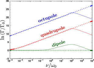
Figure 2: Comparison between numerical (full lines) and analytical (dotted lines) calculations of $\ln(\Gamma/\Gamma_{0})$ as a function of the normalized measurement rate $\nu/\omega_{0}$ for three different electric transitions: dipole ($\eta=1$, in green), quadrupole ($\eta=3$, in red) and octupole ($\eta=5$, in blue). The associated parameters used for the function $R(\omega)$ corresponding to these transitions are displayed in Table 1.

IV Experimental proposal

IV.1 Transition choice

The search for a possible candidate to observe the AZE is framed by experimental constraints. Even if the AZE is expected to be observable on magnetic dipolar transitions and even more effective on electric octupolar transitions, the very long natural lifetime (of the order of one year or more) of the excited states involved in these transitions makes them very inappropriate to lifetime measurement. Therefore, in what follows, we focus on demonstrating the AZE on an electric quadrupolar transition.

The first choice candidate to confirm the predictions derived for hydrogenic atoms is the hydrogen atom itself, by transferring the atomic population to the lowest $D$-state (the $3D$-state would play the role of the excited state $\ket{\mathrm{e}}$), and frequently monitoring the excited state. A major limit lies in the level scheme of hydrogen which allows an atom in the $3D$-state to decay to the $2P$-states by a strong dipolar transition. The lifetime of the $3D$-state is then conditioned by its dipolar coupling to $2P$ and is not limited by its quadrupolar coupling to $1S$. Therefore, no measurable reduction of the lifetime due to the AZE is expected. The same problem arises with Rydberg states, which were originally proposed as promising candidates Kofman and Kurizki (2000) for AZE observation due to their transitions in the microwave domain that favor the scaling in $(1/\omega_{0})^{\eta}$ of Eq. (10) compared to optical frequencies.

To circumvent this problem of unwanted transitions, it is then essential to identify a metastable $D$-state, which has no other decay route to the ground state than the quadrupolar transition. This can be found in the alkali-earth ions like Ca⁺ or Sr⁺, where the lowest $D$ level is lower in energy than any $P$-level. The order of magnitude of the lifetime of these $D$-levels ranges from 1 ms to 1 s. The contribution to the $D$-level spontaneous emission rate of two-photon decay, allowed by second-order perturbation theory based on non-resonant electric-dipole transitions, has been calculated in Safronova et al. (2010, 2017) for Ca⁺ and Sr⁺. The results show that the two-photon decay channel contributes to 0.01% to the lifetime of the lowest $D$-states of Ca⁺ and Sr⁺. As a consequence, the spontaneous emission from the lowest $D$-level in Ca⁺ and Sr⁺ can be considered to be due only to electric quadrupolar transition and we then focus on these two atomic systems in the following.

IV.2 Measurement scheme and read-out

Concerning the measurements of the frequently monitored excited state, ideal instantaneous projections on $\ket{\mathrm{e}}$ are not strictly required. Indeed, they amount in effect to dephasing the level $\ket{\mathrm{e}}$, that is, make the phase of state $\ket{\mathrm{e}}$ completely random Kofman and Kurizki (2000). Different schemes were proposed to emulate projective measurements in Refs. Kofman and Kurizki (2000, 2001); Ai et al. (2013) and performed in Ref. Harrington et al. (2017), for which Eq. (1) still holds. Here, we propose an alternative protocol in the same spirit of the “dephasing-only measurement” of Ref. Harrington et al. (2017). In this scheme, state $\ket{\mathrm{e}}$ is the metastable state $D_{5/2}$ and the dephasing measurement is driven by the transition from $D_{5/2}$ to $D_{3/2}$, by two lasers through the strong electric dipolar transitions to the common excited state $P_{3/2}$ (see Fig. 3) using a stimulated Raman adiabatic passage (STIRAP) process Kuklinski et al. (1989). If the two-photon Raman condition is fulfilled (identical detuning for the two transitions), the intermediate $P_{3/2}$-state is not populated and the population is trapped in a coherent superposition of the two states $D_{5/2}$ and $D_{3/2}$. By changing the laser power on each transition with appropriate time profile and time delay, the atomic population can be transferred between the two metastable $D$-states, like demonstrated in Ref. Sørensen et al. (2006). After one transfer and return, state $\ket{\mathrm{e}}$ thus acquires a phase related to the phase of the two lasers. By applying a random phase jump on one laser between each completed STIRAP transfer, the phase coherence of the excited state $\ket{\mathrm{e}}$ is washed out, and a “dephasing” measurement of the level $\ket{\mathrm{e}}$ is performed.

To measure the effective lifetime of the $D_{5/2}$-state, the read-out of the internal state must be based on electronic states which do not interfere with $D_{5/2}$. For that purpose, the electron-shelving scheme first proposed by Dehmelt can be used Dehmelt (1975). It requires two other lasers, coupling to the $S_{1/2}\to P_{1/2}$ and to the $D_{3/2}\to P_{1/2}$ transitions (see Fig. 3). When shining these two lasers simultaneously, the observation of scattered photons at the $S_{1/2}\to P_{1/2}$ transition frequency is the signature of the decay of the atom to the ground state Kreuter et al. (2005). This read-out scheme is switched on during a short time compared to the lifetime of the $D_{5/2}$-state, at a time when the STIRAP process has brought back the electron to $D_{5/2}$.

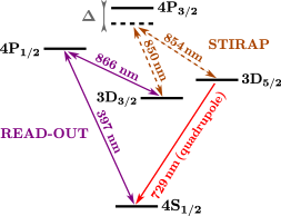
Figure 3: Dephasing measurement and read-out schemes for AZE observation in ⁴⁰Ca⁺. The transition used for the AZE is the electric quadrupole transition at $729\,\text{nm}$ (red solid arrow). The dephasing measurement can be performed using a STIRAP process between the $D_{5/2}$ and $D_{3/2}$ states via two strong electric dipole transitions $D_{5/2}\to P_{3/2}$ at $854\,\text{nm}$ and $D_{3/2}\to P_{3/2}$ at $850\,\text{nm}$, both detuned from resonance (brown dashed arrows) Sørensen et al. (2006). The read-out consists in observation of laser induced fluorescence if the atom has decayed to the ground state Dehmelt (1975) (purple solid arrows).

IV.3 Calculation for ⁴⁰Ca⁺

We now try to see whether the AZE might be observable in Ca⁺, which is not strictly speaking hydrogenic, but is alkali-like in a sense that it has a single valence electron, and can be seen as a single electron orbiting around a core with a net charge $+2e$. Ca⁺ is the lightest of the alkali-earth ions having the appropriate level-scheme required for the proposed experimental protocol (see Fig. 3). Therefore, we assume that it still makes sense to use Eq. (10) (derived for hydrogen-like atoms) and we apply it to the electric quadrupole ($\eta=3$) transition $3D_{5/2}\to 4S_{1/2}$ to find

$$\frac{\Gamma-\Gamma_{0}}{\Gamma_{0}}=A\,\frac{\nu}{\omega_{0}}\left(\frac{\omega_{\mathrm{X}}}{\omega_{0}}\right)^{2}$$ (11)

where the numerical pre-factor $A$ cannot be computed for such an electronic system (see Appendix  C for a calculation of $A$ in the simpler case of hydrogen-like atoms).

To be observable, the AZE must induce a lifetime reduction larger than 1%, the best precision reached in recent $3D_{5/2}$-lifetime measurements in Ca⁺ Kreuter et al. (2005). We evaluate $\omega_{\mathrm{X}}$ using Eq. (5) with $n_{\mathrm{g}}=4$ and $n_{\mathrm{e}}=3$ and by replacing the atomic number $Z$ by the effective number of charges $Z_{\text{eff}}=2$. Using the frequency of this transition $\omega_{0}=2\pi\times 411$ THz, this gives a ratio $(\omega_{\mathrm{X}}/\omega_{0})^{2}\simeq 6.6\cdot 10^{6}$. If the unknown pre-factor $A$ is assumed to be of the order of unity, one would need $\nu\sim 4\,\text{MHz}$ to meet the observation requirement.

The transfer between the states $D_{5/2}$ and $D_{3/2}$ has been demonstrated in ⁴⁰Ca⁺ with a STIRAP process Sørensen et al. (2006), where a complete one-way transfer duration of 5 $\mu$s was observed for 420 mW/mm² on the 850 nm $3D_{3/2}\to 4P_{3/2}$ transition and 640 mW/mm² on the 854 nm $3D_{5/2}\to 4P_{3/2}$ transition, with both lasers detuned by $\Delta=600$ MHz from resonance (see Fig. 3). To reduce the duration of the dephasing measurement to time scale smaller than 1 $\mu$s, one can increase the laser intensity by stronger focusing and/or larger power, but we can also consider that a complete STIRAP transfer is not required to achieve a dephasing of the excited state. Furthermore, a close inspection of Tables i@ and ii@ in Ref. Seke (1994) suggests that the pre-factor $A$ could be much larger than unity, making the constraint on a high measurement rate less stringent for AZE observation.

Even if the experimental requirements for AZE observation on quadrupole transition in Ca⁺ are more demanding than today’s best achievements, realistic arguments show that they can be met in a dedicated experimental set-up. This experimental challenge would benefit from theoretical insight concerning the still unknown pre-factor scaling the lifetime reduction.

V Conclusion

Based on well-established results for hydrogen-like atoms, we derived an analytical expression of the decay rate modified by frequent measurements which allows us to highlight the main condition for an observable AZE in atomic radiative decay in free space: all transitions except electric-dipole transitions will exhibit an AZE under sufficiently rapid repeated measurements. This analytical formula also indicates how the AZE scales with the measurement rate. We then identified a suitable level scheme in the alkali-earth ions Ca⁺ and Sr⁺ for AZE observation, involving the electric quadrupole transition between $D_{5/2}$ and $S_{1/2}$, and using a new “dephasing” measurement protocol based on the STIRAP technique. Other suitable experimental schemes might exist, and we encourage further proposals in this sense.

Appendix A Form of the reservoir coupling spectrum for hydrogen-like atoms in free space

Using the notations introduced in Sec. III.1, the reservoir coupling spectrum (2) is given by

$$R(\omega)=\sum_{J,M,\lambda}\hbar^{-2}\rho\left(\omega\right)\\ \times|\bra{n_{\mathrm{e}},l_{\mathrm{e}},m_{\mathrm{e}};0}\hat{H}_{I}\ket{n_{\mathrm{g}},l_{\mathrm{g}},m_{\mathrm{g}};J,M,\lambda,\omega}|^{2}.$$ (12)

Here, the density of states is $\rho\left(\omega\right)=1$, on account of the normalisation $\braket{J,M,\lambda,\omega\mid J^{\prime},M^{\prime},\lambda^{\prime},\omega^{\prime}}=\delta_{JJ^{\prime}}\delta_{MM^{\prime}}\delta_{\lambda\lambda^{\prime}}\delta\left(\omega-\omega^{\prime}\right)$ (this can be understood by dimensional considerations). In the non-relativistic approximation, Seke calculated in Seke (1994) the exact matrix elements $\bra{n_{\mathrm{e}},l_{\mathrm{e}},m_{\mathrm{e}};0}\hat{H}_{I}\ket{n_{\mathrm{g}},l_{\mathrm{g}},m_{\mathrm{g}};J,M,\lambda,\omega}$ for hydrogen-like atoms in free space, using the interaction Hamiltonian (in SI units)

$$\hat{H}_{I}=\frac{e}{m_{e}}\,\mathbf{\hat{A}}\left(\mathbf{\hat{x}}\right)\cdot\mathbf{\hat{p}}\;,$$ (13)

with $e$ the elementary electric charge, $m_{e}$ the electron mass, $\mathbf{\hat{x}}$ and $\mathbf{\hat{p}}$ the position and the linear momentum operators of the electron respectively and $\mathbf{\hat{A}}$ the vector potential operator of the quantized EM field. By employing these exact matrix elements (Eqs. (17-19) in Seke (1994)) in Eq. (12), one gets the following analytical form for the reservoir coupling spectrum

$$R(\omega)=\sum_{J,M,\lambda}\hbar^{-1}(-\mathrm{i})^{2J+2\epsilon}\alpha^{4}m_{e}c^{3}\\ \times\braket{l_{\mathrm{g}},J,m_{\mathrm{g}},M}{l_{\mathrm{g}},J,l_{\mathrm{e}},m_{e}}^{2}\\ \times\frac{\left(\frac{\omega}{\omega_{\mathrm{X}}}\right)^{2J+2\epsilon-1}}{\left[1+\left(\frac{\omega}{\omega_{\mathrm{X}}}\right)^{2}\right]^{2(n_{\mathrm{g}}+n_{\mathrm{e}}-1)}}\left(\sum_{r=0}^{N_{J}^{\prime}}d_{Jr}^{\prime}\left(\frac{\omega}{\omega_{\mathrm{X}}}\right)^{2r}\right)^{2}$$ (14)

where $c$ the speed of light in vacuum, $\alpha$ is the fine structure constant of electrodynamics, $\braket{l_{\mathrm{g}},J,m_{\mathrm{g}},M}{l_{\mathrm{g}},J,l_{\mathrm{e}},m_{\mathrm{e}}}$ are the Clebsch-Gordan coefficients of the transition of interest, and $\omega_{\mathrm{X}}$ is the non-relativistic cutoff frequency given by Eq. (5). The coefficients $d_{Jr}^{\prime}$ are numerical coefficients that have been calculated for certain transitions in Seke (1994) (note that the coefficients $d_{Jr}^{\prime}$ here correspond to the coefficients $d_{00}d_{r}$ in Eq. (18) in Ref. Seke (1994)). The index at which the sum is terminated is $N_{J}^{\prime}=n_{\mathrm{e}}+n_{\mathrm{g}}-2-(1/2)(J-l_{\mathrm{e}}-l_{\mathrm{g}}-\epsilon)$ with $\epsilon=0$ for electric transitions and $\epsilon=1$ for magnetic transitions. Eq. (14) can be recast in the form

$$R(\omega)=\sum_{J,M,\lambda}\hbar^{-1}(-\mathrm{i})^{2J+2\epsilon}\alpha^{4}m_{\mathrm{e}}c^{3}\\ \times\braket{l_{\mathrm{g}},J,m_{\mathrm{g}},M}{l_{\mathrm{g}},J,l_{\mathrm{e}},m_{\mathrm{e}}}^{2}\\ \times\sum_{r=0}^{N_{J}}d_{Jr}\frac{\left(\frac{\omega}{\omega_{\mathrm{X}}}\right)^{2J+2\epsilon-1+2r}}{\left[1+\left(\frac{\omega}{\omega_{\mathrm{X}}}\right)^{2}\right]^{2(n_{\mathrm{g}}+n_{\mathrm{e}}-1)}}$$ (15)

where $N_{J}=2\left(n_{\mathrm{e}}+n_{\mathrm{g}}\right)-4-J-l_{\mathrm{e}}-l_{\mathrm{g}}-\epsilon$ and $d_{Jr}$ are combinations of the previous $d_{Jr}^{\prime}$ coefficients. Moreover, as a consequence of the conservation of the angular momentum, the values of $J$ and $M$ must verify

$$\left\{\begin{array}[]{ll}J=|l_{\mathrm{e}}-l_{\mathrm{g}}|,|l_{\mathrm{e}}-l_{\mathrm{g}}|+1,...,|l_{\mathrm{e}}+l_{\mathrm{g}}|\\[5.69054pt] M=m_{\mathrm{e}}-m_{\mathrm{g}}\equiv\overline{M}\end{array}\right.$$ (16)

which are the exact selection rules. Therefore, the full reservoir takes the form

$$R(\omega)=\sum_{J=|l_{\mathrm{e}}-l_{\mathrm{g}}|}^{|l_{\mathrm{e}}+l_{\mathrm{g}}|}\sum_{M,\lambda}\hbar^{-1}(-\mathrm{i})^{2J+2\epsilon}\alpha^{4}m_{\mathrm{e}}c^{3}\\ \times\braket{l_{\mathrm{g}},J,m_{\mathrm{g}},M}{l_{\mathrm{g}},J,l_{\mathrm{e}},m_{\mathrm{e}}}^{2}\,\delta_{M\overline{M}}\\ \times\sum_{r=0}^{N_{J}}d_{Jr}\frac{\left(\frac{\omega}{\omega_{\mathrm{X}}}\right)^{2J+2\epsilon-1+2r}}{\left[1+\left(\frac{\omega}{\omega_{\mathrm{X}}}\right)^{2}\right]^{2(n_{\mathrm{g}}+n_{\mathrm{e}}-1)}}$$ (17)

which can be recast in the expression given in the main text by Eq. (4), where we introduced dimensionless coefficients $D_{Jr}$ involving the Clebsch-Gordan coefficients and the other constants and the sums over $M$ and $\lambda$.

Appendix B Derivation of the AZE scaling in the simple case of the reservoir (6)

Here we derive an analytical form of the integral of Eq. (1) with the simplified form of the reservoir (6). Keeping in mind the hierarchy $\omega_{0}\ll\omega_{\mathrm{X}}$, we will proceed to derive an approximate analytical expression of the general integral

$$I_{\eta\mu}\left(\tau\right)=\tau\int_{0}^{+\infty}\mathrm{d}\omega\,\frac{\omega^{\eta}}{\left[1+\left(\frac{\omega}{\omega_{\mathrm{X}}}\right)^{2}\right]^{\mu}}\sin\!\mathrm{c}^{2}\left(\left(\omega-\omega_{0}\right)\frac{\tau}{2}\right)$$ (18)

in terms of which the measurement-modified decay rate (1) is straightforwardly expressed: $\Gamma_{\tau}=DI_{\eta\mu}\left(\tau\right)/\omega_{\mathrm{X}}^{\eta-1}$. Using the binomial expansion of $\omega^{\eta}$, we first rewrite our integral as

$$I_{\eta\mu}\left(\tau\right)=\tau\sum_{k=0}^{\eta}\frac{\eta!}{k!\left(\eta-k\right)!}\omega_{0}^{\eta-k}\\ \times\int_{0}^{+\infty}\mathrm{d}\omega\,\frac{\left(\omega-\omega_{0}\right)^{k}}{\left[1+\left(\frac{\omega}{\omega_{\mathrm{X}}}\right)^{2}\right]^{\mu}}\sin\!\mathrm{c}^{2}\left(\left(\omega-\omega_{0}\right)\frac{\tau}{2}\right).$$ (19)

The $k=0$ and $k=1$ terms in the sum may be treated in a specific way. Namely, we make the following approximation of the square cardinal sine function in $F_{\tau}(\omega)$, that is illustrated in Fig. 1 (b):

$$\mathrm{sinc}^{2}\left(\left(\omega-\omega_{0}\right)\frac{1}{2\nu}\right)\simeq\left\{\begin{array}[]{ll}1\text{ for }\omega_{0}-\pi\nu<\omega<\omega_{0}+\pi\nu\;,\\[5.69054pt] 0\text{ otherwise}.\end{array}\right.$$ (20)

This approximation is sufficient for $k=0$ and $k=1$ only, as the integrand in (19) decays sufficiently fast when one moves away from $\omega_{0}$ so that the frequency ranges outside the door function (20) can be ignored. In addition to this, in the frequency range of interest here (that is, a small range of width $\sim\nu$ centered on $\omega_{0}$), we can consider that $\omega/\omega_{\mathrm{X}}\sim 0$ (which is justified by the hierarchy $\omega_{0}\ll\omega_{\mathrm{X}}$). Using these approximations, we can write the low-$k$ contribution to the integral as

$$\tau\sum_{k=0}^{1}\frac{\eta!}{k!\left(\eta-k\right)!}\omega_{0}^{\eta-k}\\ \times\int_{0}^{+\infty}\mathrm{d}\omega\,\frac{\left(\omega-\omega_{0}\right)^{k}}{\left[1+\left(\frac{\omega}{\omega_{\mathrm{X}}}\right)^{2}\right]^{\mu}}\sin\!\mathrm{c}^{2}\left(\left(\omega-\omega_{0}\right)\frac{\tau}{2}\right)\\ \simeq\tau\sum_{k=0}^{1}\frac{\eta!}{k!\left(\eta-k\right)!}\omega_{0}^{\eta-k}\int_{\omega_{0}-\pi\nu}^{\omega_{0}+\pi\nu}\mathrm{d}\omega\,\left(\omega-\omega_{0}\right)^{k}\\ =2\pi\,\omega_{0}^{\eta}.$$ (21)

Now we turn to the terms for which $k\geq 2$ and that will only exist if $\eta>1$. For these terms, replacing the square cardinal sine by a rectangle function is no longer valid, as the growth of $\left(\omega-\omega_{0}\right)^{k}$ is not overridden by the decrease of $\left(\omega-\omega_{0}\right)^{-2}$ that comes from the square cardinal sine, and therefore we must consider the whole frequency range. We therefore need to find another way to approximate the integral (19), and we may simply replace the square sine by its mean value $1/2$ here to get

$$\sin\!\mathrm{c}^{2}\left(\left(\omega-\omega_{0}\right)\frac{1}{2\nu}\right)\simeq\frac{2\nu^{2}}{(\omega-\omega_{0})^{2}}.$$ (22)

Also note, that we should not have $\omega_{0}/\nu$ excessively large, lest the square cardinal sine converges to the Dirac $\delta$ distribution, and replacing the square sine with its average value is no longer valid. We then compute the resulting integral, which, in the limit $\omega_{0}/\omega_{\mathrm{X}}\rightarrow 0$, acceptable for the transitions that interest us, reads

$$\int_{0}^{+\infty}\mathrm{d}\omega\,\frac{\left(\omega-\omega_{0}\right)^{k-2}}{\left[1+\left(\frac{\omega}{\omega_{\mathrm{X}}}\right)^{2}\right]^{\mu}}\\ \simeq\frac{1}{2}\omega_{\mathrm{X}}^{k-1}\,B\left(\frac{1-k}{2}+\mu,-\frac{1-k}{2}\right)$$ (23)

where $B$ refers to Euler’s Beta function. As can be checked from (19) and (23), of all the contributions for $k\geq 2$, the one for which $k=\eta$ is easily the largest (this is due, again, to the hierarchy $\omega_{0}\ll\omega_{\mathrm{X}}$). As such, we can rewrite (19) as

$$I_{\eta\mu}\left(t\right)\simeq 2\pi\,\omega_{0}^{\eta}+\nu\,\omega_{\mathrm{X}}^{\eta-1}\,B\left(\frac{1-\eta}{2}+\mu,-\frac{1-\eta}{2}\right)$$ (24)

where the second summand on the r.h.s. of (24) will only exist for $\eta>1$. Comparison with the natural decay rate $\Gamma_{0}=2\pi R(\omega_{0})\simeq 2\pi D\omega_{0}^{\eta}/\omega_{\mathrm{X}}^{\eta-1}$ (as $\omega_{0}\ll\omega_{\mathrm{X}}$) yields

$$\frac{\Gamma_{\tau}}{\Gamma_{0}}\simeq 1+\frac{1}{2\pi}\frac{\nu}{\omega_{0}}\\ \times\left(\frac{\omega_{\mathrm{X}}}{\omega_{0}}\right)^{\eta-1}B\left(\frac{1-\eta}{2}+\mu,-\frac{1-\eta}{2}\right).$$ (25)

Note that this result had been (partially) obtained in Kofman and Kurizki (2000), where the authors found that for a reservoir of the form $R(\omega)\propto\omega^{\eta}$ with $\eta>1$: $\Gamma\propto\nu\,\omega^{\eta-1}_{\mathrm{X}}$, in the approximation $\omega^{\eta}_{0}/\omega^{\eta-1}_{\mathrm{X}}\ll\nu\ll\omega_{\mathrm{X}}$ (cf. Eq. (20) in Ref. Kofman and Kurizki (2000)).

Appendix C Derivation of the AZE scaling in the complete case of the reservoir (4)

In this section, we extend the previous result found for a reservoir of the simple form (6) to the general form (4). Let us first sum over $r$, and then over $J$. In the generic case, the FGR decay rate will be, for the reservoir coupling spectrum (4), given by

$$\Gamma_{0J}=D_{J0}2\pi\frac{\omega_{0}^{\eta_{J}}}{\omega_{\mathrm{X}}^{\eta_{J}-1}}.$$ (26)

This is true unless $D_{J0}$ vanishes. This is the case for instance of the electric dipole transitions ($\epsilon=0$, $J=1$) between levels sharing the same principal quantum number (see Table i@ in Ref. Seke (1994)), due to the special properties of these dipolar transitions. That $D_{J0}$ vanishes can be shown rather easily by using the orthogonality properties of the Gegenbauer polynomials (see Ref. Podolsky and Pauling (1929) for a derivation of the momentum-space wave functions of hydrogen in terms of these polynomials). However, we do not focus on this special case here. In the generic case ($D_{J0}\neq 0$), the decay rate under frequent observations for a specific $J$ will be

$$\Gamma_{\tau J}\simeq 2\pi\,D_{J0}\,\frac{\omega_{0}^{\eta_{J}}}{\omega_{\mathrm{X}}^{\eta_{J}-1}}+\nu\times\sum_{r=0}^{N_{J}}D_{Jr}\,\theta\left(\eta_{J}+2r-\frac{3}{2}\right)\\ \times\,B\left(\frac{1-\eta_{J}-2r}{2}+\mu,-\frac{1-\eta_{J}-2r}{2}\right).$$ (27)

with $\theta$ the Heaviside step function. It thus appears that, for given $J$, all terms in the sum over $r$ in (4) have a contribution to the modified decay rate that is of the same order of magnitude. All that remains to be done is to sum over $J$. This sum is resolved quite differently for the free decay rate on the one hand, and the modified decay rate on the other. Namely, for the former, we see from (26) that the hierarchy $\omega_{0}\ll\omega_{\mathrm{X}}$ ensures that the contribution from the smallest possible $J$ is dominant. This value is equal to $\left|\l_{\mathrm{e}}-l_{\mathrm{g}}\right|\equiv J_{\mathrm{min}}$, and we will write $\eta_{\mathrm{min}}\equiv\eta_{J_{\mathrm{min}}}$. For the latter, however, we are forced to keep the double sum over $J$ and $N_{J}$: all (sufficiently large) powers of the frequency in the coupling contribute to the modified decay rate on the same level, with numerical prefactors as the sole difference. Namely, writing $\Gamma_{0}=\sum_{J=\left|l_{\mathrm{e}}-l_{\mathrm{g}}\right|}^{l_{\mathrm{e}}+l_{\mathrm{g}}}\Gamma_{0J}$ and $\Gamma_{\tau}=\sum_{J=\left|l_{\mathrm{e}}-l_{\mathrm{g}}\right|}^{l_{\mathrm{e}}+l_{\mathrm{g}}}\Gamma_{\tau J}$, we have obtained

$$\frac{\Gamma_{\tau}}{\Gamma_{0}}\simeq 1+\frac{1}{2\pi}\frac{\nu}{\omega_{0}}\left(\frac{\omega_{\mathrm{X}}}{\omega_{0}}\right)^{\eta_{\mathrm{min}}-1}\sum_{J=\left|l_{\mathrm{e}}-l_{\mathrm{g}}\right|}^{l_{\mathrm{e}}+l_{\mathrm{g}}}\sum_{r=r_{0}}^{N_{J}}\frac{D_{Jr}}{D_{J_{\mathrm{min}}0}}\\ \times B\left(\frac{1-\eta_{J}-2r}{2}+\mu,-\frac{1-\eta_{J}-2r}{2}\right)$$ (28)

where we have introduced

$$r_{0}\equiv\mathrm{max}\left\{\left\lfloor\frac{3}{4}-\frac{\eta_{J}}{2}\right\rfloor,0\right\}.$$ (29)

Despite the more complicated appearance of this expression, we see that the parametric dependence of the ratio of the decay rates is independent of the details of the matrix elements: the important parameter is $\eta_{\mathrm{min}}-1$. There is a competition between $\nu/\omega_{0}\ll 1$ and $\omega_{\mathrm{X}}/\omega_{0}\gg 1$ but, for $\eta_{\mathrm{min}}\geq 3$, we can expect that the second factor will dominate, especially for low values of $Z$ [see Eq. (7)]. This second factor becomes all the more dominant for higher values of $\eta_{\mathrm{min}}$, that is, for transitions with high difference between the orbital angular momenta of the initial and final levels. Only for transitions where $\left|l_{\mathrm{e}}-l_{\mathrm{g}}\right|=1$ does the second factor $\left(\omega_{\mathrm{X}}/\omega_{0}\right)^{0}=1$ fail to play a role, so that they verify $\Gamma_{\tau}\simeq\Gamma_{0}$. These transitions are often called “electric dipole transitions” (including by us in our Sec. I), although in most cases they are accompanied by emission of photons of angular momentum $J>1$ (as well of course as $J=1$). Indeed, as we have recalled with Eq. (26), it is always the photons with the smallest allowed value $J_{\mathrm{min}}$ of $J$ that dominate the spontaneous emission in an electronic transition.

References

- Kofman and Kurizki (2000) A. G. Kofman and G. Kurizki, Nature 405, 546 (2000).
- Facchi et al. (2001) P. Facchi, H. Nakazato, and S. Pascazio, Phys. Rev. Lett. 86, 2699 (2001).
- Misra and Sudarshan (1977) B. Misra and E. C. G. Sudarshan, J. Math. Phys. 18, 756 (1977).
- Cook (1988) R. Cook, Phys. Scr. 1988, 49 (1988).
- Itano et al. (1990) W. M. Itano, D. J. Heinzen, J. J. Bollinger, and D. J. Wineland, Phys. Rev. A 41, 2295 (1990).
- Patil et al. (2015) Y. S. Patil, S. Chakram, and M. Vengalattore, Phys. Rev. Lett. 115, 140402 (2015).
- Kaulakys and Gontis (1997) B. Kaulakys and V. Gontis, Phys. Rev. A 56, 1131 (1997).
- Kofman and Kurizki (1996) A. G. Kofman and G. Kurizki, Phys. Rev. A 54, R3750 (1996).
- Lewenstein and Rza̧żewski (2000) M. Lewenstein and K. Rza̧żewski, Phys. Rev. A 61, 022105 (2000).
- Fischer et al. (2001) M. C. Fischer, B. Gutiérrez-Medina, and M. G. Raizen, Phys. Rev. Lett. 87, 040402 (2001).
- Harrington et al. (2017) P. M. Harrington, J. T. Monroe, and K. W. Murch, Phys. Rev. Lett. 118, 240401 (2017).
- Moses (1973) H. Moses, Phys. Rev. A 8, 1710 (1973).
- Seke (1994) J. Seke, Phys. A 203, 269 (1994).
- Cohen-Tannoudji et al. (1989) C. Cohen-Tannoudji, J. Dupont-Roc, and G. Grynberg, Photons and atoms: introduction to quantum electrodynamics (Wiley Online Library, 1989).
- Zheng et al. (2008) H. Zheng, S. Y. Zhu, and M. S. Zubairy, Phys. Rev. Lett. 101, 200404 (2008).
- Ai et al. (2010) Q. Ai, Y. Li, H. Zheng, and C. P. Sun, Phys. Rev. A 81, 042116 (2010).
- Zhou et al. (2017) Z. Zhou, Z. Lü, H. Zheng, and H.-S. Goan, Phys. Rev. A 96, 032101 (2017).
- Chaudhry (2016) A. Z. Chaudhry, Sci. Rep. 6, 29597 (2016).
- Facchi and Pascazio (1998) P. Facchi and S. Pascazio, Phys. Lett. A 241, 139 (1998).
- Debierre et al. (2015) V. Debierre, T. Durt, A. Nicolet, and F. Zolla, Phys. Lett. A 379, 2577 (2015).
- Safronova et al. (2010) M. S. Safronova, W. R. Johnson, and U. I. Safronova, Journal of Physics B: Atomic, Molecular and Optical Physics 43, 074014 (2010).
- Safronova et al. (2017) M. S. Safronova, W. R. Johnson, and U. I. Safronova, Journal of Physics B: Atomic, Molecular and Optical Physics 50, 189501 (2017).
- Kofman and Kurizki (2001) A. G. Kofman and G. Kurizki, Phys. Rev. Lett. 87, 270405 (2001).
- Ai et al. (2013) Q. Ai, D. Xu, S. Yi, A. G. Kofman, C. P. Sun, and F. Nori, Sci. Rep. 3 (2013).
- Kuklinski et al. (1989) J. R. Kuklinski, U. Gaubatz, F. T. Hioe, and K. Bergmann, Phys. Rev. A 40, 6741 (1989).
- Sørensen et al. (2006) J. L. Sørensen, D. Møller, T. Iversen, J. B. Thomsen, F. Jensen, P. Staanum, D. Voigt, and M. Drewsen, New J. Phys. 8, 261 (2006).
- Dehmelt (1975) H. Dehmelt, in Bull. Am. Phys. Soc., Vol. 20 (1975) p. 60.
- Kreuter et al. (2005) A. Kreuter, C. Becher, G. P. T. Lancaster, A. B. Mundt, C. Russo, H. Häffner, C. Roos, W. Hänsel, F. Schmidt-Kaler, R. Blatt, and M. S. Safronova, Phys. Rev. A 71, 032504 (2005).
- Podolsky and Pauling (1929) B. Podolsky and L. Pauling, Phys. Rev. 34, 109 (1929).