Fluid simulations of plasma turbulence at ion scales:
comparison with Vlasov-Maxwell simulations

Abstract

Comparisons are presented between a hybrid Vlasov-Maxwell (HVM) simulation of turbulence in a collisionless plasma and fluid reductions. These include Hall-magnetohydrodynamics (HMHD) and Landau fluid (LF) or FLR-Landau fluid (FLR-LF) models that retain pressure anisotropy and low-frequency kinetic effects such as Landau damping and, for the last model, finite Larmor radius (FLR) corrections. The problem is considered in two space dimensions, when initial conditions involve moderate-amplitude perturbations of a homogeneous equilibrium plasma subject to an out-of-plane magnetic field. LF turns out to provide an accurate description of the velocity field up to the ion Larmor radius scale, and even to smaller scales for the magnetic field. Compressibility nevertheless appears significantly larger at the sub-ion scales in the fluid models than in the HVM simulation. High frequency kinetic effects, such as cyclotron resonances, not retained by fluid descriptions, could be at the origin of this discrepancy. A significant temperature anisotropy is generated, with a bias towards the perpendicular component, the more intense fluctuations being rather spread out and located in a broad vicinity of current sheets. Non-gyrotropic pressure tensor components are measured and their fluctuations are shown to reach a significant fraction of the total pressure fluctuation, with intense regions closely correlated with current sheets.

I Introduction

Turbulence represents a complex and fascinating phenomenon ubiquitous in nature. It can be observed from simple fluids to plasmas, with compelling evidence in space plasmas observations, as well as in laboratory devices. The dynamics can be envisioned as a cascade of energy through different scales: energy is injected at large scales through inhomogeneities, and is then transferred self-consistently towards smaller scales, until dissipation processes become relevant. Although in classical fluids this behavior is relatively well understood, in more exotic systems like plasmas, the cascade process is more ‘controversial’ and, even though it has been matter of study for many decades, it is far from being completely understood.

In fluid systems, as described by Kolmogorov, under the assumption of isotropy and time stationarity, turbulence exhibits an universal behavior Kolmogorov (1941). Plasmas, that can be described as a fluid of particles, obey to a similar Kolmogorov description of the dynamics, at least at scales large compared to the ion gyroradius. However, while energy is transferred to small scales, plasmas manifest their kinetic nature. With kinetic we mean here all the processes that cannot be described by usual collisional fluids. Characterizing the limitations of the fluid description of turbulence is of crucial relevance for understanding and modeling plasma dynamics.

Thanks to the contributions from space missions it is possible to benefit from a large amount of data to investigate the dynamics of a natural plasma, the solar wind, which can be used as a real plasma laboratory. In situ observations show that the interplanetary medium is in a state of fully developed turbulence Bruno & Carbone (2013). The energy is injected at large scales, where the turbulent spectrum is dominated by Alfvénic fluctuations, characterized by a high correlation between magnetic and velocity fields and by incompressibility Belcher & Davis (1971). In the inertial range, the turbulence spectra display power laws, reminiscent of the typical behavior of fluids Matthaeus & Goldstein (1982); Tu & Marsch (1995). However, around ion characteristic scales, a break in the spectral slope is observed, with the appearance (beyond a possible narrow transition range Sahraoui et al. (2010)) of steeper spectra extending down to the electron scales Leamon et al. (1998, 2000); Bale et al. (2005); Smith et al. (2006); Bourouaine et al. (2012); Alexandrova et al. (2012); Saharaoui et al. (2013); Matthaeus et al. (2014) and an enhancement of magnetic compressive fluctuations Alexandrova et al. (2007, 2008); Hamilton et al. (2008); Salem et al. (2012); Kiyani et al. (2013); Perrone et al. (2016, 2017). In this short-wavelength range, often named dissipation range, plasma dynamics is sensitive to Hall dispersion and ion finite Larmor radius (FLR) effects, together with Landau damping and cyclotron resonances. Moreover, spacecraft measurements reveal that the solar wind is far from the classical thermodynamical equilibrium, the particle distribution functions being characterized by non-Maxwellian effects. In particular, ion velocity distributions show strong temperature anisotropies, with a preferential perpendicular heating and accelerated particles in the direction parallel to the ambient magnetic field Marsch (2006).

Plasma turbulence appears as a very complex interaction between turbulent electromagnetic fields, macroscopic flows, pressure anisotropy and other non-thermal effects. Although different physical mechanisms, such as ion-cyclotron resonance (e.g., Hollweg & Isenberg (2002)), Landau damping (e.g., Valentini et al. (2005); Schekochihin et al. (2009)), particle energization close to current sheets and reconnection sites Retinò et al. (2007); Sundkvist et al. (2007); Osman et al. (2011); Chasapis et al. (2015, 2017), enhancement of collisions Pezzi et al. (2016); Pezzi (2017) or stochastic heating (e.g., Chandran et al. (2010)), have been proposed to explain in situ observations, the role of dissipation in collisionless plasmas is still not well understood.

Nowadays numerical simulations represent an indispensable tool to understand the nonlinear dynamics of plasma behavior in different environments. Due to the large time scale separation between ion and electron dynamics, simulations that can cover the whole range of scales of a plasma system are very challenging. Such fully kinetic simulations are not really feasible with the available computational resources, and certain sets of approximations are needed.

In the study of solar wind turbulence, different numerical models have been used, with vastly different assumptions and numerical schemes. The simplest fluid-like approach is given by magnetohydrodynamics (MHD) (e.g., Gurnett & Bhattacharjee (2005)) and all the related models that include different corrections and/or asymptotics, such as reduced MHD (e.g., Zank & Matthaeus (1992)), Hall MHD (e.g., Ghosh & Goldstein (1997)), electron MHD (e.g., Kingsep et al. (1987); Gordeev et al. (1994); Cho & Lazarian (2004)), electron reduced MHD (e.g., Schekochihin et al. (2009)). Other fluid-like approaches include Landau fluid (e.g., Snyder et al. (1997)) and FLR-Landau fluids (Sulem & Passot (2015) and references therein). A simplified Vlasov-Maxwell approach, where the gyro-motion of the particles is averaged out from the system, thus restricting the dynamics to low-frequency phenomena, is given by gyrokinetic codes (e.g., Brizard & Hahm (2007); Howes et al. (2006); Numata et al. (2010)). For a more complete kinetic description of the plasma, the most adopted numerical approach is represented by the Particle In Cell (PIC) methods Birdsall & Langdon (1985). Hybrid PIC simulations (e.g., Parashar et al. (2009)) treat ions as particles and electrons as a neutralizing fluid, while full PIC codes (e.g., Karimabadi et al. (2013)) describe both ions and electrons as kinetic particles. An alternative method to the PIC approach is provided by the Eulerian Vlasov model Mangeney et al. (2002); Valentini et al. (2005, 2007). Recently, an hybrid Vlasov-Maxwell (HVM) code has been extensively used for the analysis of the kinetic effects in the solar wind turbulent plasma Valentini et al. (2008); Valentini & Veltri (2009); Valentini et al. (2010, 2011); Perrone et al. (2011); Servidio et al. (2012); Perrone et al. (2013, 2014a, 2014b); Valentini et al. (2014); Servidio et al. (2014a, 2015); Vásconez et al. (2014); Valentini et al. (2016); Pezzi et al. (2017a, b). The main advantage of HVM simulations is that the level of noise is negligible and the small-scale effects can be described with reasonable accuracy.

Even though several studies have been done using various approaches, most of the results are obtained starting with different initial conditions or plasma parameters, thus making the comparison difficult. A comparative analysis of different plasma models and codes, simulating the same initial conditions for turbulence, and under the same plasma parameters, is required to understand the nature of different features recovered in turbulent systems Henri et al. (2013); Parashar et al. (2015). In the present paper we focus on the properties of collisionless plasma turbulence, by a comparative study of three different plasma models, from fluid-like approximations to a self-consistent kinetic treatment of collisionless plasmas. In particular, we use (i) compressible Hall MHD (HMHD), (ii) FLR-Landau fluid (FLR-LF), and (iii) hybrid Vlasov-Maxwell (HVM) simulations, with the same geometry and initial conditions. The conditions of the simulations are constrained by the difficulty of performing kinetic simulations of developed turbulence on the present-day computers. We thus resorted to consider a periodic two-dimensional spatial domain and to assume relatively strong perturbations of a homogeneous equilibrium state in order to limit the size and duration of the simulations, although the considered fluid modeling of kinetic effects assumes weak perturbations.

The paper is organized as follows. In Section II, we briefly describe the three models we have considered, namely HMHD, LF or FLR-LF and HVM. In Section III, comparisons between the predictions of HVM with HMHD and LF are presented for a simulation with cold electrons, focusing on the electromagnetic field, the ion velocity (discriminating in particular between the solenoidal and compressible contribution to the in-plane component) and, beyond the HMHD description, temperature anisotropy, and heat fluxes. Section IV discusses properties of nongyrotropic pressures within HVM and also within a FLR-LF simulation with warm electrons ($\beta_{e}=1$). A few concluding remarks are made in Section V.

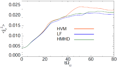
Figure 1: Averaged out-of-plane squared current density $\langle j_{z}^{2}\rangle$ versus time for HMHD (green line), LF (blue line) and HVM (red line) simulations.

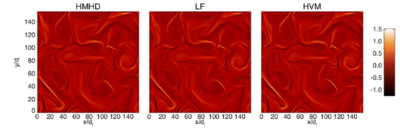
Figure 2: Color scale plot of the out-of-plane current density $j_{z}$ for Hall MHD (left), LF (middle) and HVM (right) simulations at $t=60$.

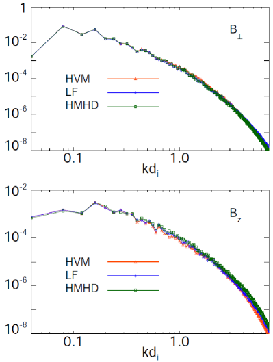
Figure 3: Spectra of the in-plane ${\mathbf{B}}_{\perp}$ (top) and out-of-plane $B_{z}$ magnetic field components, for HMHD (green solid-square line), LF (blue solid-diamond line) and HVM (red solid-triangle line) simulations at $t=60$.

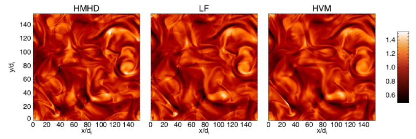
Figure 4: Color scale plot of the out-of-plane magnetic fluctuations for HMHD (left), LF (middle) and HVM (right) simulations at $t=60$.

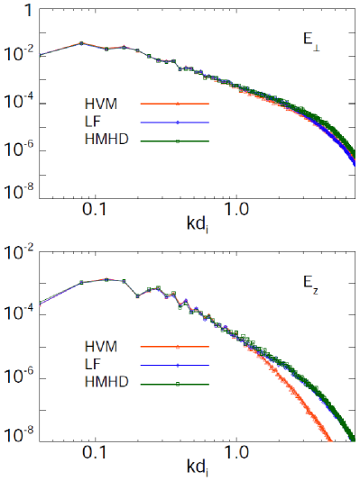
Figure 5: Spectra of in plane and out-of-plane plasma electric field for HMHD (green solid-square line), LF (blue solid-diamond line) and HVM (red solid-triangle line) simulations at $t=60$.

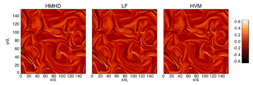
Figure 6: Color scale plot of the out-of-plane vorticity $\omega_{z}$ for HMHD (left), LF (middle) and HVM (right) simulations at $t=60$.

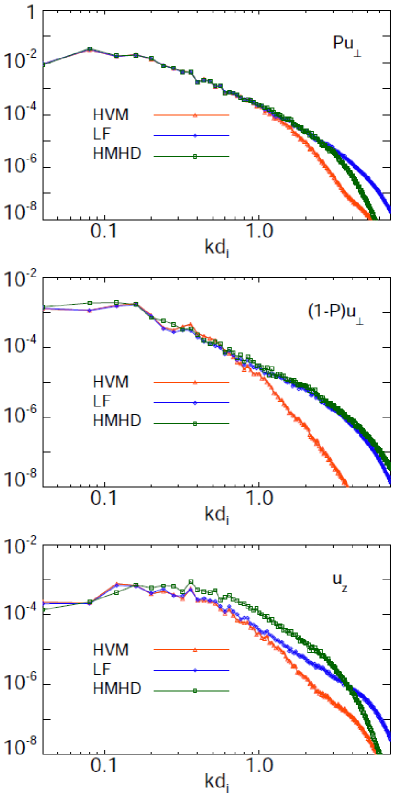
Figure 7: Spectra of the solenoidal $P{\mathbf{u}}_{\perp}$ (top) and compressible $(1-P){\mathbf{u}}_{\perp}$ (middle) components of the in-plane velocity, and of out-of-plane velocity $u_{z}$ (bottom) for HMHD (green solid-square line), LF (blue solid-diamond line) and HVM (red solid-triangle line) simulations at $t=60$.

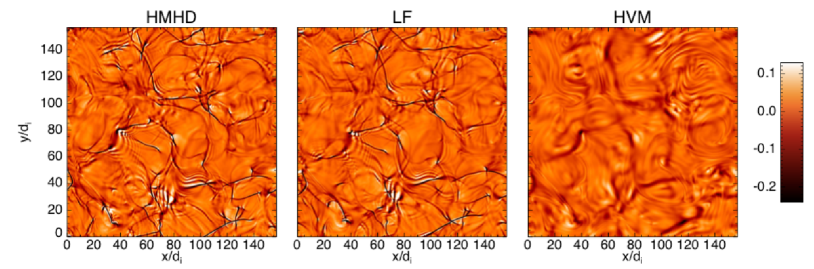
Figure 8: Color scale plot of the ion velocity divergence $\xi={\bf\nabla}\cdot{\mathbf{u}}$ for HMHD (left), LF fluid (middle) and HMV (right) simulations at $t=60$.

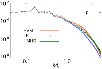
Figure 9: Spectra of plasma density $\rho$ for HMHD (green solid-square line), LF (blue solid-diamond line) and HVM (red solid-triangle line) simulations at $t=60$.

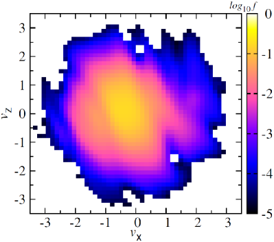
Figure 10: Color scale plot of the proton velocity distribution in the $v_{x}$–$v_{z}$ plane at the end of HVM simulation.

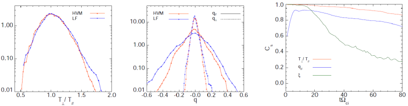
Figure 11: PDFs of the ion temperature anisotropy, $T_{\perp}/T_{\parallel}$ (left), parallel, ${q}_{\parallel}$ (solid lines), and perpendicular, ${q}_{\perp}$ (dashed lines), heat flux in the reference frame of the local magnetic field (middle) for LF (blue-diamond line) and HVM (red-triangle line) simulations at $t=60$. Right panel shows the time evolution of the the Spearman correlation coefficient between LF and HVM results for the proton temperature anisotropy (red line), parallel heat flux (blue line) and compressibility (green line).

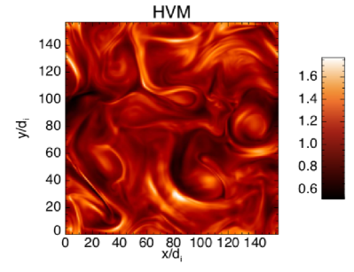
Figure 12: Color scale plot of the temperature anisotropy $T_{\perp}/T_{\|}$ for the HVM run at $t=60$.

II The models

The dynamical behavior of plasma fluctuations depends markedly on their frequencies. At the lowest frequencies, ions and electrons are locked together by electrostatic forces and the plasma behaves like an electrically conducting fluid; this is the MHD. Note that, when collisions are sufficiently weak, pressure anisotropy can also develop. At somewhat higher frequencies, electrons and ions can move relatively to each other, behaving like two separate and interpenetrating fluids; this is the two-fluid regime. At still higher frequencies, a kinetic theory, where the statistical description of the plasma state is provided by the particle distribution functions in phase space, is required.

In this section, we provide a description of the models used in the present paper. The simplest treatment is given by HMHD that retains dispersive effects which become significant at scales comparable to the ion skin depth $d_{i}$. Then, we focus on FLR-LF, that also retains pressure anisotropy and low-frequency kinetic effects such as Landau damping and finite Larmor radius corrections at scale comparable to or smaller than the ion gyroradius. When the latter effect is neglected, we refer to the model as LF. Finally, we describe the HVM approach, where the evolution of the ions is obtained by solving an equation for the ion distribution function. Electron inertial effects have been included in all three cases with a mass ratio $m_{i}/m_{e}=100$. Both in fluid and HVM simulations, electrons are treated as a cold fluid. The case of a FLR-LF simulation with a warm isothermal electron fluid with $\beta_{e}=1$ is also considered since, as discussed below, the cold electron FLR-LF simulation can only be integrated up to an intermediate time after which numerical difficulties in the calculations of the FLR terms are encountered. The results of Section III thus involve a precise comparison between HMHD, HVM and LF simulations. The discussion of FLR corrections in the warm case is presented in Section IV.

In both fluid and kinetic simulations, at t=0, the equilibrium consists of a homogeneous plasma embedded in a uniform background magnetic field, $\bm{B}_{0}$, along the $z$-direction. In the HVM run, ion distribution function is initialized with a Maxwellian with homogeneous density. The system evolution is investigated in a double periodic domain $(x,y)$ perpendicular to $\bm{B}_{0}$. The equilibrium configuration is initially perturbed by velocity and magnetic field fluctuations with wavenumbers in the range $0.08<k<0.24$ in units of $d_{i}^{-1}$, where $k=2\pi m/L$, with $2\leq m\leq 6$ (here $L$ being the box size in each spatial direction). The phases of these perturbations are random. The rms of the magnetic perturbations is $\delta b/B_{0}\sim 0.3$ and neither density disturbances nor parallel variances are imposed at $t=0$. The ion plasma beta is $\beta_{i}=1$, defined as $2v_{th,i}^{2}/v_{A}^{2}$, where $v_{th,i}=\sqrt{T_{i}/m_{i}}$ is the ion thermal speed and $v_{A}=B_{0}/\sqrt{4\pi n_{0}m_{i}}$ the Alfvén speed. The system size in the spatial domain is $L=2\pi\times 25d_{i}$ in both $x$ and $y$ directions, discretized with $1024^{2}$ grid-points in the 2D spatial domain. For the HVM run, the 3D velocity domain, limited by $\pm 5v_{th,i}$ in each directions, is discretized with an uniform grid of $51^{3}$ points.

II.1 Hall-MHD

The compressible HMHD equations including a modeling of electron inertia Valentini et al. (2007) read

$$\frac{\partial\rho}{\partial t}+\nabla\cdot\left(\rho\bm{u}\right)=0,$$ (1)

$$\frac{\partial\bm{u}}{\partial t}+\left(\bm{u}\cdot\nabla\right)\bm{u}=-\frac{{\beta}}{2\rho}\nabla p+\frac{1}{\rho}\left[\left(\nabla\times\bm{B}\right)\times\bm{B}\right],$$ (2)

$$\frac{\partial\bm{B}}{\partial t}=-\nabla\times\bm{E}+\eta\nabla^{2}\bm{B},$$ (3)

$$(1+\alpha\nabla^{2})\bm{E}+\left[\bm{u}\times\bm{B}-\frac{1}{\rho}\left(\nabla\times\bm{B}\right)\times\bm{B}\right]=0$$ (4)

$$p=\rho^{\gamma},$$ (5)

where $\rho$ is the plasma density (only due to ions), $\bm{u}$ the hydrodynamic velocity of the plasma, $\bm{B}$ the magnetic field, $p$ the total pressure (taken isotropic), $\gamma=5/3$ the adiabatic index, $\eta=0.02$ the magnetic diffusivity and $\alpha=1/100$ an artificial electron to ion mass ratio. Equations (1)-(5) are written in a dimensionless form. In particular, $\rho$ is normalized to $n_{0}m_{i}$; $\bm{u}$, to the Alfvén speed; $t$, to the inverse ion-cyclotron frequency $\Omega_{ci}^{-1}$ and the unit length to the ion skin depth $d_{i}$.

All the fluid numerical codes employ a 2D Fourier pseudo-spectral method to calculate spatial derivatives, and time integration is performed via a third-order Runge-Kutta scheme. Aliasing errors in the evaluation of nonlinear terms are partially removed by a 2/3 truncation in the spectral space.

II.2 Landau fluid and FLR-Landau fluid

The FLR-Landau fluid model appears as a system of dynamical equations for the magnetic field and for the density, velocity, parallel and perpendicular pressures and heat fluxes of the ions. The electric field is given by a generalized Ohm’s law which includes the Hall term, the electron pressure gradient (when present), together with electron inertia with the same simplified form as in the HMHD case. The fluid hierarchy is closed by expressing the gyrotropic fourth-rank moments in terms of the above quantities, in a way consistent with the low-frequency linear kinetic theory. Two cases will be considered. In the simple LF case, ion linear Landau damping only is retained while the FLR-LF case also takes into account FLR corrections. These corrections are evaluated algebraically in terms of the retained quantities. The equations are too complicated to be explicitly written here, but can be found in Sulem & Passot (2015), namely in Section 2 (where the terms corresponding to the work of the nongyrotropic pressure force are neglected), in Eqs. (3.22) and (3.23) and in Subsections 5.1.1-5.1.4. A main assumption for modeling Landau damping (and thus closing the fluid hierarchy) is that, up to the distortion of the magnetic field lines, Landau damping keeps the same form as in the linear regime, an hypothesis which requires that the turbulence fluctuations are not too strong (a condition which is unfortunately not met in the simulations presented in this paper). This modeling involves a Hilbert transform along the distorted magnetic field lines which leads to Landau dissipation. Its approximation in the numerical code is discussed in Passot et al. (2014). FLR-LF accuracy was successfully tested in the linear regime in three space dimensions, in particular at the level of the dispersion relation, the damping and the polarization of kinetic Alfvén waves (e.g., Hunana et al. (2013)). Three-dimensional simulations of kinetic Alfvén wave turbulence using this model are presented in Kobayashi et al. (2017). In the present two-dimensional regime, the situation is more delicate, as the ambient field does not affect the transverse dynamics, making Landau damping only due to the transverse distortion of the magnetic field lines.

II.3 Hybrid Vlasov-Maxwell

We solve the Vlasov-Maxwell equations in the hybrid approximation (kinetic ions and fluid electrons) by using the HVM code Valentini et al. (2007), in a 2D3V phase space domain (two dimensions in physical space and three dimensions in velocity space). The Vlasov equation is integrated for the ion distribution function, while the electron response is taken into account through a generalized Ohm’s law for the electric field. The dimensionless HVM equations are given by

$$\frac{\partial f}{\partial t}+\bm{v}\cdot\frac{\partial f}{\partial\bm{r}}+\left(\bm{E}+\bm{v}\times\bm{B}\right)\cdot\frac{\partial f}{\partial\bm{v}}=0,$$ (6)

supplemented by Eqs. (3)-(4), where $f(\bm{r},\bm{v},t)$ is the ion distribution function. The ion density, $n$, and the bulk velocity, $\bm{u}$, are evaluated as velocity moments of the ion velocity distribution. The quasi-neutrality approximation, $n=n_{i}=n_{e}$, is used and cold electrons are considered. As in the previous models, time is scaled by the inverse ion-cyclotron frequency, $\Omega_{ci}^{-1}$; velocity by $v_{A}$; lengths by the ion skin depth, $d_{i}=v_{A}/\Omega_{ci}$; and masses by the ion mass, $m_{i}$. From now on, all physical quantities will be expressed in units of the characteristic parameters listed above.

The numerical solution of the Vlasov equation is based on the well-known time splitting method, first proposed in Cheng & Knorr (1976). The time splitting consists in separating the evolution of the particle distribution function in phase space into subsequent translations, first in physical space and then in velocity space Mangeney et al. (2002). Finally, the Current Advance Method (CAM) Matthews (1994); Valentini et al. (2007) provides numerical solutions for the time advancement of electric and magnetic fields. The time step, $\Delta t$, has been chosen in such a way that the Courant-Friedrichs-Lewy condition for the numerical stability of the Vlasov algorithm is satisfied Peyret & Taylor (1986). It is to be noted that the monocore computer time per time step on machines of comparable speed is roughly 450 time larger for the Vlasov simulation than for the FLR-LF run.

III Comparisons of HMHD, LF and HVM simulations

Large-scale fluctuations produce a turbulent cascade toward kinetic scales, as in the fluid counterpart. In analogy with fluid models for plasma in decaying turbulence Mininni & Pouquet (2009), it exists an instant of time, $t^{*}$, at which the turbulence reaches its maximum activity. Near this particular time, decaying turbulence shares many statistical similarities with steady state (driven) turbulence. It is possible to identify $t^{*}$ by following the temporal evolution of the averaged out-of-plane squared current density $\langle j_{z}^{2}\rangle$, which is a good indicator of the level of the turbulent activity. It is important to note that the maximum value of $\langle j_{z}^{2}\rangle$ is prescribed by the strength of the dissipation processes. All simulations include a magnetic diffusivity term with a coefficient $\eta=2\times\cdot 10^{-2}$. In the fluid runs, additional regularizing terms are to be supplemented to smooth the equations and produce a similar behavior of $\langle j_{z}^{2}\rangle$. For this purpose, we add a hyperviscosity and an hyperdiffusivity, as bi-Laplacians, with coefficients $\nu_{4}=\eta_{4}=5\times 10^{-4}$ in the case of HMHD and $\nu_{4}=\eta_{4}=10^{-4}$ for LF In the latter model, bi-Laplacian dissipative terms are also added, with a coefficient equal to $2.5\times 10^{-3}$ in the equations for the density and the pressures, and $10^{-4}$ in the equations for the heat fluxes in order to deal with the high level of compressibility in the simulation (the Mach number reaching values up to $0.4$). Note that all the above dissipative terms have been added only for numerical reasons, in order to prevent spurious effects such as artificial filamentation of current sheets and shock-like structures. However, we verified that these non-ideal contributions are only important at wavenumbers $k$ such that at $kd_{i}>3$, thus at scales significant smaller than the turbulent inertial range. This high-precision tuning of the artificial dissipation terms, achieved through several convergence tests, is particularly important for fluid models that, even in their extensions retaining Landau damping, do not capture all the dissipative processes acting at the kinetic scales.

Figure 1 shows the behavior of $\langle j_{z}^{2}\rangle$ as a function of time for the corresponding HMHD (green line), LF (blue line) and HVM (red line) simulations. This color code will be used in all the other graphs presented in this paper. The similarity between the turbulence activity in the different models permits comparisons between these descriptions. Note also that the same $\beta$ parameter was used for the three simulations, thus ensuring a similar level of density fluctuations (as can be checked below by inspection of the density spectrum). Whereas there is no ambiguity in the choice of $\beta$ for the LF and HVM runs, since they both share the same linear theory, for HMHD no proper choice of $\beta$ would however permit to recover the same linear theory. Consequences will be discussed below at the level of the velocity field divergence.

III.1 Turbulence and coherent structures

	HMHD/LF	HMHD/HVM	LF/HVM
$b_{x}$	99%	99%	99%
$b_{y}$	99%	99%	99%
$b_{z}$	82%	80%	93%
$j_{z}$	90%	85%	91%
$e_{x}$	94%	94%	97%
$e_{y}$	94%	92%	96%
$e_{z}$	89%	90%	96%
$\rho$	85%	80%	92 %
$u_{x}$	95%	95%	98%
$u_{y}$	96%	96%	99%
$u_{z}$	67%	49%	83%
$\omega_{z}$	86%	82%	90%
$\xi$	9%	31 %	35%

Table 1: Spearman correlation coefficients between several quantities of the three runs, i.e. HMHD/LF (left column), HMHD/HVM (center column) and LF/HVM (right column), at $t=60$.

	LF/ HVM
$p_{\perp}$	92 %
$p_{\|}$	89 %
$T_{\perp}$	91 %
$T_{\|}$	88 %
$T_{\perp}/T_{\|}$	92 %
$q_{\perp}$	37 %
$q_{\|}$	79 %

Table 2: Spearman correlation coefficients between the kinetic quantities of the LF and HVM simulations at $t=60$.

Turbulence leads to the generation of coherent structures, such as current and vorticity sheets. Figure 2 displays, for the three models, a color plot of the out-of-plane current density, $j_{z}=(\nabla\times{\bf B})_{z}$ at time $t=60$, during the period of maximal turbulence activity. Note that in this figure and in all the other color scale plots presented in this paper, the extremal values of the fields can exceed the limits of the color bar ranges in some very localized regions. This choice was made in order to improve the visibility of the structures of intermediate amplitude. Comparison between HMHD (left panel), LF (center panel) and HVM (right panel) simulations shows that there are strong similarities regarding the in-plane magnetic field. Regions of very intense $j_{z}$ are in particular present in each panels at the same locations.

In order to get a more quantitative assessment of the similarity between the three runs in physical space, we evaluate at $t=60$ the Spearman correlation coefficients, defined as

$$C_{s}(f,g)=\frac{\sum_{i}(Rf_{i}-\bar{f})(Rg_{i}-\bar{g})}{\sqrt{\sum_{i}(f_{i}-\bar{f})^{2}}\sqrt{\sum_{i}(g_{i}-\bar{g})^{2}}}\$$ (7)

where $f_{i}$ and $g_{i}$ are the values at the grid points of the same scalar field provided by different models at a given time, $R$ is an operator ranking these values in a decreasing order, and $\bar{f}$ and $\bar{g}$ denote the mean values of the corresponding fields at the considered time. An overview of the values of correlation $C_{s}$ for various fields between the three runs, i.e. HMHD/LF, HMHD/HVM and LF/HVM, at $t=60$, is reported in Table 1. More specifically, we obtained for the out-of-plane current a correlation coefficient of $85\%$ for HMHD/HVM and $91\%$ for LF/HVM. This result indicates a high correlation at the level of the in-plane magnetic field. For $B_{x}$ and $B_{y}$, the correlation is indeed of $99\%$ both HMHD/HVM and LF/HVM.

For a Fourier space characterization of the in-plane magnetic field in the three models, we plot in Fig. 3 (top panel) the energy spectra of the in-plane components ${\mathbf{B}}_{\perp}$ of the magnetic field fluctuations. We observe that these spectra are very close for the three models up to $kd_{i}=5$.

In order to analyze the out-of-plane magnetic fluctuations $B_{z}$, we display in Fig. 4 the color plot of this field in the three models. In spite of a global similarity, discrepancies are visible at small scales. A conspicuous difference concerns the presence of steepened waves-like features (probably associated with fast waves) in the fluid runs, which are absent (or at least heavily damped) in the Vlasov case. The coefficient $C_{s}$ is indeed $80\%$ for HMHD/HVM and $93\%$ for LF/HVM. The difference between the three runs are also visible on the energy spectrum shown in Fig. 3 (bottom panel), for wavenumber close to $kd_{i}=1$, LF being slightly closer to HVM than HMHD is.

It is also of interest to compare the electric field given by the various descriptions, as it is commonly measured by satellite missions and is at the origin of particle acceleration, although in the numerical simulations it is constructed from various other fields by means of the generalized Ohm’s law. Analysis in physical space shows that all three components display correlation coefficients larger than $90\%$ and $96\%$ for HMHD/HVM and LF/HVM respectively. The spectrum of the in-plane electric field displayed in Fig. 5 are similar throughout the whole spectrum for the three descriptions, the agreement LF/HVM being slightly better than HMHD/HVM. For the out of plane component, both fluid descriptions disagree with HVM result for $kd_{i}>1$.

Turning to the velocity field, we first plot in Fig. 6 the out-of-plane vorticity $\omega_{z}$ at $t=60$ obtained with the three models. A good similarity is observed, supported by the results of correlation measurements (see Table 1), implying a good agreement at the level of the (dominant) solenoidal part of the in-plane velocity. In Fourier space, the energy spectrum of this field, displayed in Fig 7 (top panel), reveals a satisfactory match between both fluid models and HVM up to $kd_{i}=1$.

Although significantly smaller than the solenoidal part (a factor $4$ in the rms values), the compressible component of the in-plane velocity is very different in the three simulations, as visible on the corresponding color plots of $\xi=\nabla\cdot{\mathbf{u}}$ in Fig. 8. Both for HMHD/HVM and LF/HVM, the correlation coefficient of $\xi$ is of order $30\%$. The HVM large-scale behavior of $\xi$ is relatively well reproduced with the fluid simulations. On the other hand, the small-scales in HVM are smoothed out, thus explaining this intermediate value of the correlation. The poor agreement between HMHD and LF is rather due to the fact that the small-scale features of the fluid simulations are completely out of phase due to a difference in the description of the fast waves linear behavior, as mentioned in Sec. II. Shock-like cellularization, typical of compressible turbulence and evidently due to an higher in-plane magnetosonic activity, is quite clear in HMHD and LF models. The fronts are significantly mollified in HVM. This difference suggests that most likely, in a fully kinetic treatment, compressible activity is balanced by Landau damping (approximately modeled in LF) and ion cyclotron absorption (beyond the fluid description), which evidently will induce other effects such as temperature anisotropy, heat flux, and beams formations in the velocity distribution function. Indeed, the spectrum of the compressible part of the velocity displayed in Fig. 7 (middle panel) for each of the simulations shows a rapid decay at $kd_{i}>1$ in the case of HVM, while HMHD and LF spectra are very similar and decay more slowly.

The different behavior between the compressible and solenoidal parts of the velocity is also conspicuous on the correlation of the out-of plane velocity $u_{z}$, which is $49\%$ only between HMHD and HVM, while it reaches $83\%$ between LF and HVM. This is confirmed by inspection of the corresponding spectra displayed in Fig. 7 (bottom panel). LF and HVM are rather close up to $kd_{i}\sim 1$, while the HMHD spectrum is quite different, even at $kd_{i}<1$. In order to understand this behavior, we performed an extra simulation within the bi-adiabatic approximation (i.e. with zero heat fluxes). It is interesting to note that the corresponding $u_{z}$ spectrum agrees with HVM up to roughly $kd_{i}=0.7$ (not shown) and then deviates significantly to catch up the HMHD spectrum. This indicates that at large scales, pressure anisotropy is a dominant correction, while at smaller scales, Landau damping plays a dominant role and contributes to reduce compressiblity Hunana et al. (2011).

At the level of the plasma density, correlations of $80\%$ and $92\%$ are respectively obtained in the cases HMHD/HVM and LF/HVM. The corresponding spectra, displayed in Fig. 9, show a larger amplitude of the fluctuations for HVM at scales immediately smaller than $d_{i}$, a feature possibly related to the flattening of the density spectrum found in space plasma observations Alexandrova et al. (2013) but not reproduced with fluid models.

It is interesting at this stage to consider the ion distribution function. Figure 10 shows that it is significantly distorted in the $(v_{x},v_{z})$ -plane, with the presence of rings probably associated with ion-cyclotron absorption. This could be an explanation for the sharp decay of the compressible velocity spectrum that fluid models are unable to capture.

III.2 Kinetic effects

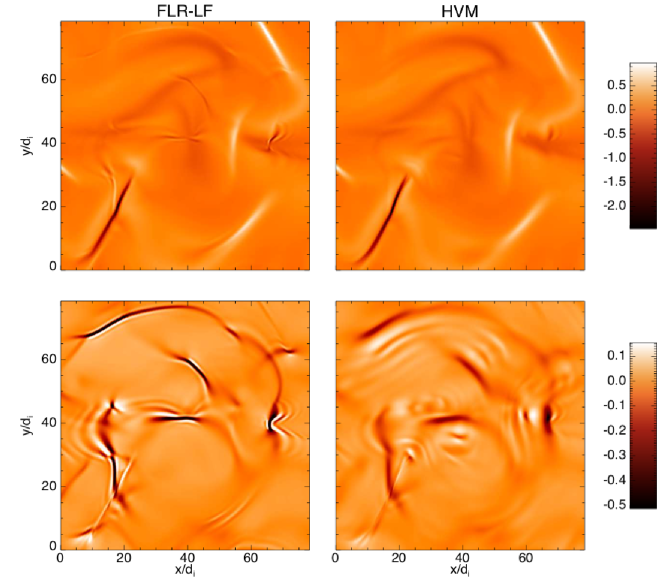
Figure 13: Zoom of the out-of-plane current density $j_{z}$ (top) and proton velocity divergence $\xi$ (bottom) for the FLR-LF simulation with $\beta_{e}=0$ (left) and HVM (right) simulations at $t=25$.

In the last decades, several studies of turbulent collisionless plasmas, through in situ observations and numerical simulations, have shown that particle distribution functions are far from the typical configuration of thermodynamical equilibrium Marsch (2006); Servidio et al. (2012); Perrone et al. (2013, 2014a, 2014b); Valentini et al. (2014); Servidio et al. (2014a, 2015); Vásconez et al. (2014); Valentini et al. (2016). Temperature anisotropy, particle heating and acceleration are observed in turbulence, localized in and near coherent structures. Thanks to kinetic approaches, and in particular to HVM simulations, we have the possibility to study in detail the non-Maxwellian effects on the ion velocity distribution. On the other hand, the LF and FLR-LF models provide information on the low-frequency kinetic response of the plasma in a turbulent context, missing nevertheless other kinetic effects such as the ion-cyclotron resonance. In this part, we shall focus on temperature anisotropy and ion gyrotropic heat fluxes where a precise comparison can be performed between the LF and HVM simulations at $\beta_{e}=0$. An investigation of non-gyrotropic pressure tensor components will be performed in Section IV where a FLR-LF run at $\beta_{e}=1$ will also be considered.

We start quantifying the non-Maxwellian features through the statistical analysis of the ion temperature anisotropy, $T_{\perp}/T_{\parallel}$, defined as the ratio between the ion perpendicular and parallel temperatures. The initial condition has been set up to have spatially isotropic ion temperature. During the development of turbulence, the temperature does not remain isotropic but presents local enhancements and depressions. Left panel of Fig. 11 shows the PDFs of $T_{\perp}/T_{\|}$, for both LF (blue solid-diamond line) and HVM (red solid-triangle line) simulations at $t=60$. The behavior is similar: the PDFs elongate both in the parallel $(T_{\perp}/T_{\|}<1)$ and perpendicular $(T_{\perp}/T_{\|}>1)$ directions, displaying a strong anisotropic behavior, the anisotropy being more important along the perpendicular direction. Spearman correlation of the temperature ratio between the two simulations (see Table 2) is $92\%$, similar to the correlations at the level of individual perpendicular ($91\%$) and parallel ($88\%$) temperatures.

Figure 12 displays a color plot of the temperature anisotropy $T_{\perp}/T_{\|}$ for the HVM run at $t=60$. It is interesting to note that the regions of large (or small) values are not much correlated with the locations of the current sheets. The are rather related to regions of compression or dilation in the vicinity of these coherent structures and thus appear more diffuse (see also Bañón Navarro et al. (2016); Sorriso et al. (2018, under review) for a similar observation)

We now investigate the heat flux tensor, defined as the third order moment of the ion distribution function. In particular, we look at the gyrotropic contribution characterized by the parallel $q_{\|}$ and perpendicular $q_{\perp}$ heat fluxes. The PDFs of ${q}_{\parallel}$ (solid line) and of ${q}_{\perp}$ (dashed line) for LF (in blue-diamond) and HVM (in red-triangle) simulations are reported in the middle panel of Fig. 11, at the maximum of the turbulent activity $(t=60)$. Although, ${q}_{\parallel}$ and ${q}_{\perp}$ are both picked around zero, a preferential transfer of heat flux is observed in the parallel direction. The LF and HVM results display similar distribution function. The agreement is better for the perpendicular heat flux, the PDF of the parallel heat flux being more populated for large deviation in the LF case. At the level of the Spearman correlation coefficients, the tendency is however opposite, with $37\%$ and $79\%$ for $q_{\perp}$ and $q_{\|}$ respectively. This difference in the quality of the correlations is very probably related to the hierarchy closure which, for technical reasons, involves a Padé approximant of the plasma response function of higher order for the parallel than for the perpendicular quantities.

Figure 11 (right panel) shows the time evolution, from $t=1$, of the Spearman correlation coefficient between LF and HVM simulations for the proton temperature anisotropy (red line), parallel heat flux (blue line) and velocity divergence (green line). After a brief transient in the case of the heat fluxes originating from the low-frequency assumption underlying the hierarchy closure, a decreasing behavior is recovered for all the quantities. In particular, both the runs start with an isotropic condition for ions, $T_{\perp}=T_{\parallel}$, and the correlation is 1. Due to the development of the turbulence, the ion distribution starts to deform, with generation of temperature anisotropy and heat flux, especially in the parallel direction. Both runs are able to describe this physics. However, due to the peculiarity of each description and to the limitation of the LF model, $C_{s}$ decreases with the increase of turbulence.

The most important discrepancy between the models appears in the compressibility. Starting from $C_{s}(\xi)=1$, the deviation becomes important very soon and, at $t=40$, the correlation is only about $50\%$.

IV The non-gyrotropic components of the pressure tensor

The previous sections were concerned with a general description of the turbulence that develops in the HMHD, LF and HVM simulations, paying particular attention to the comparison between the fluid and kinetic modelings. Apart from a general description of velocity and magnetic structures together with their associated power spectra, kinetic features such as temperature anisotropy and heat fluxes have been discussed. The most important difference is related to the excess of small-scale kinetic compressibility in the fluid simulations as opposed to what is observed in the HVM simulation. It is now of interest to discuss the properties of the non-gyrotropic pressure tensor, comparing the outcome of HVM and FLR-LF simulations and also investigating how their amplitude relates to the current sheets. Whereas for the LF case no numerical issue other than the necessity of adding hyperdiffusivity to the density, pressure and heat flux equations was encountered, in the FLR-LF case it was not possible to continue the simulation past $t=30$ without having to use unreasonably large coefficients. There is probably not a unique reason for this numerical issue but one can mention that the high-order velocity derivatives present in the FLR terms are sensitive to sharp gradients. The Mach number of the $\beta_{e}=0$ simulation is large (the rms Mach number at $t=60$ reaches $0.39$), permitting the development of rather strong shocks in the FLR-LF run, as revealed by the sharp dark lines in the plot of the velocity divergence at $t=25$ (see left bottom panel of Fig. 13). These shocks do not preclude to continue the simulation. The numerical difficulty is rather related to the destabilization of a current sheet after it has interacted with a traveling shock. Bottom left corner of the panels for $\nabla\cdot\bm{u}$ and $j_{z}$ in Fig. 13 (left panel) shows such an interaction happening for the FLR-LF run. In the HVM simulation, these shocks are mollified and hardly visible at the level of the current sheet (right panels of Fig. 13). Other smooth oscillations are nevertheless present in the Vlasov case. This is consistent with the previous remark concerning the difference between the HVM and the LF simulation at the level of the compressible part of the velocity field.

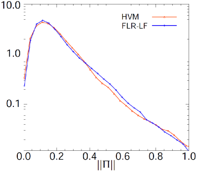
Figure 14: PDFs of the norm of the non-gyrotropic tensor, $||{\mathbf{\Pi}}||$ for FLR-LF (blue solid-diamond line) and HVM (red solid-triangle line) simulations at $t=60$.

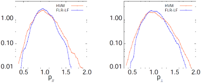
Figure 15: PDFs of gyrotropic pressure components, $p_{\|}$ and $p_{\perp}$ (left and right), for FLR-LF (blue solid-diamond line) and HVM (red solid-triangle line) simulations at $t=60$.

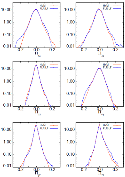
Figure 16: PDFs of the various non-gyrotropic tensor components, ${\mathbf{\Pi}}_{xx}$ and ${\mathbf{\Pi}}_{xy}$ (top left and right), ${\mathbf{\Pi}}_{xz}$ and ${\mathbf{\Pi}}_{yy}$ (middle left and right) and ${\mathbf{\Pi}}_{yz}$ and ${\mathbf{\Pi}}_{zz}$ (bottom left and right) for FLR-LF (blue solid-diamond line) and HVM (red solid-triangle line) simulations at $t=60$.

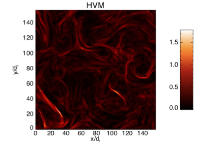
Figure 17: Color scale plot of the norm of the non-gyrotropic pressure tensor $||{\mathbf{\Pi}}||$ for the HVM run at $t=60$

IV.1 Comparison with a FLR-LF simulation at $\beta_{e}=1$

As will be seen, the FLR pressure tensor is weakly sensitive to the value of the electron beta parameter (at least as long as no strong shocks form), justifying a comparison between the HVM simulation (at $\beta_{e}=0$) and a FLR-LF simulation performed at $\beta_{e}=1$. Indeed, due to a lower value of the Mach number, a FLR-LF run at $\beta_{e}=1$ can be completed without too much difficulty, but nevertheless at the expense of using larger hyperviscosity coefficients (note also that a comparison with a HVM at $\beta_{e}=1$ would be interesting but not presently possible due to computational power limitations). This comparison also contributes to a validation of the FLR formulation used in the FLR-LF model.

Before displaying the FLR pressure tensor components, let us recall some definitions. The pressure tensor can be written as

$${\bf p}={\bf p^{G}}+{\bf\Pi}\ ,$$ (8)

where ${\bf p^{G}}$ the gyrotropic pressure tensor (built from the parallel $p_{\|}$ and perpendicular $p_{\perp}$ pressures) and ${\bf\Pi}$ is due to the FLR effects. The pressure tensor, together with its gyrotropic and nongyrotropic components are symmetric, with the additional condition ${\rm tr}({\bf\Pi})=0$. Note that all the FLR pressure tensor components are calculated in a basis using the direction of the local magnetic field.

Figure 14 shows the PDFs of the norm of ${\bf\Pi}$ for both FLR-LF (with $\beta_{e}=1$; blue solid-diamond line) and HVM (with $\beta_{e}=0$; red solid-triangle line) simulations at $t=60$. The norm is defined as

$$||{\bf\Pi}||=\sum_{i,j}|{\bf\Pi}_{ij}|\ ,$$ (9)

where the sum includes all components. Both simulations show that the contribution of the non-gyrotropic term to the total pressure is not negligible and that the distribution functions are very similar. This surprising result reveals that the FLR pressure tensor is not very sensitive to the Mach number (in particular the compressible component of the velocity). The PDF of the gyrotropic components is however more directly influenced by a difference in the $\beta_{e}$ parameter of the two simulations, as demonstrated in Fig. 15 showing a greater deviation between the two runs.

Although there is no point in making more precise comparisons between the two runs which use different values of the $\beta_{e}$ parameter, let us mention that the Spearman correlation FLR-LF/HVM for $||{\bf\Pi}||$ is $49\%$.

When considering the PDFs of the individual cartesian components of the non-gyrotropic pressure tensor, we note that the components involving a $z$ index are more peaked (see Fig. 16). As previously noted for the norm, a surprisingly good agreement is found between the FLR-LF and the HVM simulations, demonstrating that the fluid modeling captures the essential properties of the non-gyrotropic pressure tensor.

Moreover, a dependence of $||{\bf\Pi}||$ on the level of turbulence has been observed (not shown here). Indeed, it increases when the magnitude of the turbulent fluctuations increases in the system, reaching its maximum when turbulent activity is maximum ($t=60$). Figure 17 shows a color plot of $||{\bf\Pi}||$ from the HVM run at $t=60$. It indeed seems rather well correlated with the out-of-plane current although displaying multiple filamentary structures where the current only shows isolated sheets. A very similar picture is obtained with the FLR-LF run (not shown).

V Conclusion

Two-dimensional simulations of turbulence development in a collisionless plasma subject to an out-of-plane ambient magnetic field were performed using HVM and fluid models such as HMHD, LF and FLR-LF. Both in HVM and LF, electrons are cold, but an extra FLR-LF simulation with $\beta_{e}=1$ is used to illustrate the comparison of the non-gyrotropic pressure tensor between FLR-LF and HVM. In all the cases, initial conditions are large-scale, moderate-amplitude perturbations of a homogeneous equilibrium state. A main observation concerns the capabilities of fluid models to approach HVM simulations, depending on the considered fields. The magnetic field is globally well described, especially the in-plane component, up to wavenumbers such that $kd_{i}\approx 5$. For the velocity field, the agreement stops at $kd_{i}=1$ for the in-plane components. The out-of-plane velocity is poorly described at all scales by HMHD, but satisfactorily reproduced by LF up to $kd_{i}\approx 1$. We checked that Landau damping contributes to this agreement. Interestingly, the compressible (in-plane) velocities of HMHD and LF are very similar and correctly reproduce HVM up to $kd_{i}\approx 1$. At this wavenumber, the HVM energy spectrum of this component displays a sharp break. Fast kinetic effects, such as ion-cyclotron resonance, not retained in fluid approaches, could be at the origin of this effect. Concerning quantities not retained by HMHD, a satisfactory agreement is obtained between LF and HVM at the level of temperature anisotropy and heat fluxes. A significant temperature anisotropy is generated, with a bias towards the perpendicular component, the more intense fluctuations being rather spread out and located in a broad vicinity of current sheets. The FLR-LF run at $\beta_{e}=1$ displays a surprisingly good agreement with HVM regarding non-gyrotropic pressure components, showing their relative insensitivity to the $\beta_{e}$ parameter. The fluctuation amplitude of these components almost reaches $50\%$ of the gyrotropic ones, with the most intense regions located near current sheets, showing the necessity of taking them into account in a small-scale modeling of the plasma.

Further developments should include comparisons in three space dimensions where linear waves, not present in two dimensions but accurately described by FLR-LF, are expected to significantly affect the dynamics.