Fluctuations of radiative heat exchange between two bodies

Abstract

We present a theory to describe the fluctuations of nonequilibrium radiative heat transfer between two bodies both in far and near-field regime. As predicted by the blackbody theory, in far field, we show that the variance of radiative heat flux is of the same order of magnitude as its mean value. However, in near-field regime we demonstrate that the presence of surface polaritons makes this variance more than one order of magnitude larger than the mean flux. We further show that the correlation time of heat flux in this regime is comparable to the relaxation time of heat carriers in each medium. This theory could open the way to an experimental investigation of heat exchanges far from the thermal equilibrium condition.

Nonequilibrium fluctuations in electronic transport Akkermans inside mesoscopic systems have been investigated in detail since the beginning of 90’s Blanter ; Beenakker . In these systems, fluctuations of electric currents were found to be of the same order of magnitude as their mean value. These fluctuations originate from coherence effects for electronic wavefunctions. An analog thermal behavior is well known for heat flux exchanged in far-field regime between two objects held at two different temperatures. This behavior is a direct consequence of blackbody fluctuations as predicted by Einstein Planck ; Einstein . Surprisingly these fluctuations have not been investigated so far at close separation distances. However, in the last two decades it has been shown that the properties of thermal radiation in the near-field regime can radically differ from that observed in the far field. Indeed in this case the thermal radiation can be quasi-monochromatic Eckardt , polarized SetalaEtAl2002 and spatially coherent Hesketh . As the radiative heat flux between two thermalized objects is concerned, it has been shown within the framework of Rytov’s fluctuational electrodynamics Rytov that it can surpass the blackbody limit by orders of magnitude PoldervH ; LoomisPRB94 ; Pendry ; JoulainSurfSciRep05 ; VolokitinRMP07 ; PBA2 ; BiehsEtAl2010 and strong deviations from the behavior observed in far-field regime have been predicted in a variety of configurations RodriguezPRL11 ; McCauleyPRB12 ; RodriguezPRB12 ; MullerarXiv ; BimontePRA09 ; KrugerPRL11 ; MessinaEurophysLett11 ; KrugerPRB12 ; MessinaPRA14 ; BimontearXiv16 ; BenAbdallahPRL11 ; ZhuPRL16 ; ZhengNanoscale11 ; MessinaPRL12 ; BenAbdallahPRL14 ; MessinaPRB13 ; BenAbdallahPRL13 ; NikbakhtJAP14 ; BenAbdallahAPL06 ; BenAbdallahPRB08 ; NikbakhtEPL15 ; BenAbdallahPRL16 ; LatellaarXiv16 . Many of these theoretical predictions have been confirmed experimentally down to few nanometer distances Hargreaves ; Kittel1 ; Chen1 ; Chen2 ; Chen3 ; Rousseau ; Ottens ; Kralik2 ; Chevrier1 ; Chevrier2 ; Pramod1 ; Pramod2 ; Lipson ; Kittel2 . So far, investigation of radiative heat exchanges between two bodies was limited to the analysis of the statistical average of the Poynting vector (PV) PoldervH ; LoomisPRB94 . To go beyond this first-order theory and to investigate the statistical properties of the near-field thermal radiation it is necessary to determine the high-order moments of fields radiated by the fluctuating sources as well as the heat flux mediated by photon tunneling. The theoretical analyzis of these moments could open, for instance, the way to the investigation of thermodynamical properties of these systems or to the study of irreversible dynamical processes related to them far from equilibrium Evans ; Evans2 ; Wang ; Garnier .

In this work, within the flutuational electrodynamics framework introduced by Rytov we derive the second-order statistical properties of thermal field radiated by a hot body. First, we show that, in the far-field regime, the standard deviation of the radiative heat flux is of the same order of magnitude as the mean value, a well-known result from the blackbody theory MandelWolf . On the contrary, in the near-field regime we find that the standard deviation of the radiative heat flux can be much higher than the mean value, although the mean value itself is in this regime orders of magnitude larger than the blackbody value. We demonstrate that this significant enhancement of the fluctuation amplitude can be observed when the medium supports surface polaritons JoulainSurfSciRep05 . Finally, we establish that in presence of such waves the correlation time CT of PV is of the same order as the relaxation time of atomic vibrations (phonons) that is much larger than the CT of blackbody radiation. We further show that for metals the amplitude of fluctuations can also be large, whereas the CT is in the far- and near-field regime of the same order as that of blackbody radiation.

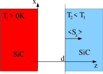
Figure 1: Sketch of the considered configuration: A SiC halfspace at temperature $T_{1}$ exchanges heat by heat radiation with a second SiC halfspace with $T_{2}<T_{1}$ in a distance $d$.

Let us start with the z-component of the mean PV describing the thermal radiation of a semi-infinite medium at temperature $T_{1}$ into another semi-infinite medium $T_{2}=0\,{\rm K}$ as sketched in Fig. 1 is given by

$${\begin{split}\langle S_{1,z}\rangle(\mathbf{r}_{d})&=\langle E_{1,x}(\mathbf{r}_{d},t)H_{1,y}(\mathbf{r}_{d},t)\rangle\\ &\quad-\langle E_{1,y}(\mathbf{r}_{d},t)H_{1,x}(\mathbf{r}_{d},t)\rangle.\end{split}}$$ (1)

Here the index $1$ symbolizes the fact that the fields are generated by the thermal sources in medium 1 and the brackets denote the ensemble average. The correlation functions (CFs) are evaluated at the interface of the second medium at $\mathbf{r}_{d}=(0,0,d)^{t}$ where the energy transfer to the second body really occurs, and at a given time $t$. Note that we are here considering a non-equilibrium steady-state situation so that the above CFs and the mean PV do not depend on time. In order to determine the second moment we can exploit the Gaussian property of the thermal fields which allows us to express the higher moments of the fields in terms of the second moments Rytov . The main assumption here is that the fluctuational field is composed of a multitude of microfields created by charge and current fluctuations from different volume elements of the medium which give similar and statistically independent contributions. The Gaussian property then follows from the central-limit theorem Rytov ; SanchezEtAl2004 . Furthermore, from the rotational symmetry we have $\langle E_{1,x}^{2}\rangle=\langle E_{1,y}^{2}\rangle$ and $\langle H_{1,x}^{2}\rangle=\langle H_{1,y}^{2}\rangle$; the components of the electric and magnetic fields are uncorrelated MandelWolf so that $\langle H_{1,x}H_{1,y}\rangle=\langle E_{1,x}E_{1,y}\rangle=0$ and $\langle E_{1,y}H_{1,y}\rangle=\langle E_{1,x}H_{1,x}\rangle=0$. Finally, the mixed CFs have the symmetry $\langle E_{1,x}H_{1,y}\rangle=-\langle E_{1,y}H_{1,x}\rangle$ SupplM . With these relations together with the Gaussian property of fields we obtain

$$\langle S_{1,z}^{2}\rangle=2\langle E_{1,x}^{2}\rangle\langle H_{1,x}^{2}\rangle+\frac{3}{2}\langle S_{1,z}\rangle^{2}$$ (2)

so that the variance $\langle\bigl{(}\Delta S_{1,z}\bigr{)}^{2}\rangle\equiv\langle S_{1,z}^{2}\rangle-\langle S_{1,z}\rangle^{2}$ of the normal component of PV reads

$$\langle\bigl{(}\Delta S_{1,z}\bigr{)}^{2}\rangle=2\langle E_{1,x}^{2}\rangle\langle H_{1,x}^{2}\rangle+\frac{1}{2}\langle S_{1,z}\rangle^{2}.$$ (3)

Obviously, this quantity is of the same order as the mean heat flux squared and by virtue of the first term on the right hand side it contains in general contributions from the electric and magnetic fields as well. As the normalized standard deviation is concerned it reads accordingly

$$\sigma_{S}\equiv\sqrt{\frac{\langle\bigl{(}\Delta S_{1,z}\bigr{)}^{2}\rangle}{\langle S_{1,z}\rangle^{2}}}=\sqrt{\frac{1}{2}+2\frac{\langle E_{1,x}^{2}\rangle\langle H_{1,x}^{2}\rangle}{\langle S_{1,z}\rangle^{2}}}.$$ (4)

Hence, we see that the standard deviation of the thermal emission of a semi-infinite medium is given by the mean value of PV and the electric and magnetic part of the mean energy density. Expression (4) can of course also be used to evaluate the standard deviation of the PV for a halfspace emitting into vacuum at $0\>K$ by replacing the permittivity of the right halfspace (i.e. $z>d$) by that of vacuum. In this case, the mean PV in the expression for the standard deviation will contain the contribution of propagating waves only, whereas the term $\langle E_{x}^{2}\rangle\langle H_{x}^{2}\rangle$ also contain the contributions of evanescent waves. A meaningful result for the fluctuations of the PV in the far-field regime can be obtained by evaluating the term $\langle E_{x}^{2}\rangle$ and $\langle H_{x}^{2}\rangle$ in the limit $d\rightarrow\infty$ or $d\gg\lambda_{\rm th}$.

In order to evaluate the standard deviation, we need to introduce the CFs of fields at arbitrary separation distances. This can be done in the the framework of the theory of fluctuational electrodynamics. To this end, we consider two halfspaces as sketched in Fig. 1 (of permittivity $\epsilon_{1}=\epsilon_{2}=\epsilon_{\rm SiC}$) separated by a vacuum gap of width $d$ having the temperatures $T_{1}\neq 0\,{\rm K}$ and $T_{2}=0\,{\rm K}$. In this case the mean value of the PV in z-direction is given by ${\langle S_{1,z}(\mathbf{r}_{d})\rangle=2\langle E_{1,x}(\mathbf{r}_{d},t)H_{1,y}(\mathbf{r}_{d},t)\rangle.}$ From the relation between the fields and the current density and using the fluctuation-dissipation theorem the CFs of electric and magnetic fields read SupplM ; Agarwal1975 ; Eckhardt1978 ; Eckhardt1979 ; Doro2011

$$\langle E_{1,x}(t)H_{1,y}(t^{\prime})\rangle =\int_{0}^{\infty}\!\!\frac{{\rm d}\omega}{2\pi}\Theta_{1}(\omega)\int\!\!\frac{{\rm d}\kappa}{2\pi}\,\kappa\frac{\gamma_{1}^{\prime}{\rm e}^{-2\gamma_{0}^{\prime\prime}d}}{2|\gamma_{1}|^{2}}$$

$$\quad\times\biggl{(}\frac{|t_{\rm s}|^{2}|1+r_{\rm s}|^{2}}{|D_{\rm s}|^{2}}{\rm Re}\bigl{(}\gamma_{1}^{*}{\rm e}^{-{\rm i}\omega\tau}\bigr{)}$$ (5)

$$\quad+\frac{|t_{\rm p}|^{2}|1-r_{\rm p}|^{2}}{|D_{\rm p}|^{2}}\frac{|\gamma_{1}|^{2}+\kappa^{2}}{|k_{1}|^{2}|\epsilon_{1}|}{\rm Re}\bigl{(}\gamma_{1}\epsilon_{1}^{*}{\rm e}^{-{\rm i}\omega\tau}\bigr{)}\biggr{)}$$

$$\langle E_{1,x}(t)E_{1,x}(t^{\prime})\rangle =\int_{0}^{\infty}\!\!\frac{{\rm d}\omega}{2\pi}\mu_{0}\omega\Theta_{1}(\omega)\cos(\omega\tau)\int\!\!\frac{{\rm d}\kappa}{2\pi}\,\kappa$$

$$\quad\times\frac{\gamma_{1}^{\prime}{\rm e}^{-2\gamma_{0}^{\prime\prime}d}}{2|\gamma_{1}|^{2}}\biggl{(}\frac{|t_{\rm s}|^{2}}{|D_{\rm s}|^{2}}\bigl{|}1+r_{s}\bigr{|}^{2}$$ (6)

$$\qquad+\frac{|t_{\rm p}|^{2}}{|D_{\rm p}|^{2}}\frac{|\gamma_{1}|^{2}+\kappa^{2}}{|k_{1}|^{2}}\frac{|\gamma_{1}|^{2}}{|k_{1}|^{2}}\bigl{|}1-r_{p}\bigr{|}^{2}\biggr{)},$$

$$\langle H_{1,x}(t)H_{1,x}(t^{\prime})\rangle =\int_{0}^{\infty}\!\!\frac{{\rm d}\omega}{2\pi}\epsilon_{0}\omega\Theta_{1}(\omega)\cos(\omega\tau)\int\!\!\frac{{\rm d}\kappa}{2\pi}\,\kappa$$

$$\quad\times\frac{\gamma_{1}^{\prime}{\rm e}^{-2\gamma_{0}^{\prime\prime}d}}{2|\gamma_{1}|^{2}}\biggl{(}\frac{|t_{\rm s}|^{2}}{|D_{\rm s}|^{2}}\frac{|\gamma_{1}|^{2}}{k_{0}^{2}}\bigl{|}1+r_{s}\bigr{|}^{2}$$ (7)

$$\qquad+\frac{|t_{\rm p}|^{2}}{|D_{\rm p}|^{2}}\frac{|\gamma_{1}|^{2}+\kappa^{2}}{k_{0}^{2}}\bigl{|}1-r_{p}\bigr{|}^{2}\biggr{)},$$

with $\tau:=t-t^{\prime}$ and the mean energy of a harmonic oscillator given by $\Theta_{1}(\omega)=\hbar\omega/\bigl{(}\exp(\hbar\omega/k_{\rm B}T_{1})-1\bigr{)}$. Here $D_{{\rm s}/{\rm p}}=|1-r_{{\rm s}/{\rm p}}^{2}{\rm e}^{2{\rm i}\gamma_{0}d}|^{2}$, $\gamma_{1}^{2}=k_{0}^{2}\epsilon_{1}-\kappa^{2}$, $\gamma_{0}^{2}=k_{0}^{2}-\kappa^{2}$, $k_{1}=\sqrt{\epsilon_{1}}k_{0}$ and $k_{0}=\omega/c$; $t_{{\rm s}/{\rm p}}$ and $r_{{\rm s}/{\rm p}}$ are the Fresnel transmission and reflection coefficients of the single interface;$\epsilon_{0}$ and $\mu_{0}$ are the permittivity and permeability of vacuum.

With these relations we can determine the fluctuations of PV between any couple of isotropic and homogeneous halfspaces considering only the thermal radiation from a single halfspace with $T_{1}\neq 0\,{\rm K}$. In particular it is possible to derive from these expressions the moments of heat flux radiated by a blackbody of temperature $T_{1}$ in vacuum. Indeed, in this case by setting the permittivity of the materials $\epsilon_{1}$ to that of vacuum, i.e. $\epsilon_{1}\equiv 1$ so that $t_{\rm s}=t_{\rm p}=1$ and $\gamma_{1}=\gamma_{0}$ then it is easy to see that SupplM

$$\langle S_{z}\rangle\equiv\langle S_{\rm BB,z}\rangle=\sigma_{\rm BB}T_{1}^{4},$$ (8)

and

$$\langle E^{2}_{x}(t)\rangle \equiv\langle E_{\rm BB,x}^{2}\rangle=c\mu_{0}\frac{2}{3}\sigma_{BB}T_{1}^{4},$$ (9)

$$\langle H^{2}_{x}(t)\rangle \equiv\langle H_{\rm BB,x}^{2}\rangle=c\epsilon_{0}\frac{2}{3}\sigma_{BB}T_{1}^{4}$$ (10)

introducing the Stefan-Boltzmann constant $\sigma_{\rm BB}$. It follows that the normalized standard deviation for the blackbody radiation reads

$$\sigma_{S,\rm BB}=\sqrt{\frac{25}{18}}$$ (11)

showing that the standard deviation of PV is of the same order as its mean value. This result is obviously consistent with the well-known deviation $\sigma=\langle I\rangle/\sqrt{2}$ of unpolarized thermal radiation, $\langle I\rangle$ being the mean value of the intensity MandelWolf .

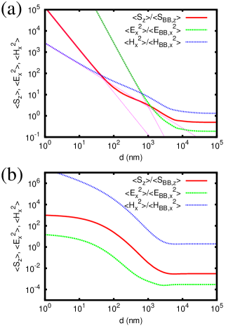
Figure 2: $\langle S_{z}\rangle$, $\langle E_{x}^{2}\rangle$ and $\langle H_{x}^{2}\rangle$ as function of gap size $d$ for two (a) SiC and (b) Au halfspaces with $T_{1}=300\,{\rm K}$ and $T_{2}=0\,{\rm K}$; all quantities are normalized to the blackbody values given in Eq. (8), (9) and (10) for $T_{1}=300\,{\rm K}$. The thin lines in (a) are the quasi-static results showing that $\langle S_{z}\rangle\propto 1/d^{2}$, $\langle E_{x}^{2}\rangle\propto 1/d^{3}$ and $\langle H_{x}^{2}\rangle\propto 1/d$ in the strong near-field regime.

Now let us pay attention to heat exchanges between two bulk samples made of silicon carbide (SiC) a polar material whose permittivity at frequency $\omega$ can be described by the Drude-Lorentz model and two samples made of gold (Au) described by the Drude model Palik (see also SupplM ). We first show in Fig. 2 plots of CFs as derived above and normalized by the CFs for a blackbody. For SiC it can be seen that in the quasi-static limit $\langle S_{z}\rangle\propto 1/d^{2}$, $\langle E_{x}^{2}\rangle\propto 1/d^{3}$, and $\langle H_{x}^{2}\rangle\propto 1/d$ due to the near-field contribution. These distance dependences are universal features in the quasi-static limit. For Au all the curves would have the corresponding distance dependences for $d\rightarrow 0$ (see SupplM ), but for the shown values of $d$ the quasi-static regime is not yet fully reached.

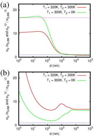
Figure 3: Normalized standard deviation $\sigma_{S}$ from Eq. (4) and Eq. (14) as function of the gap size $d$ for two (a) SiC and (b) Au halfspaces with $T_{1}=300\,{\rm K}$ and $T_{2}=0\,{\rm K}$ and $T_{1}=320\,{\rm K}$ and $T_{2}=300\,{\rm K}$. The standard deviation is normalized to the blackbody results $\sigma_{S,{\rm BB}}\approx 1.18$ from Eq. (11) and $\sigma_{S,{\rm BB}}^{12}\approx 6.25$ from Eq. (14), resp. The vertical lines are the quasi-static limits SupplM and the blackbody value.

The standard deviation $\sigma_{S}$ shown in Fig. 3(a) for SiC and in Fig. 3(b) for Au is $d$ independent in the far-field regime (i.e. $d\gg\lambda_{\rm th}$) as can be expected from the fact that the CFs are $d$ independent in this case. Since SiC is a very good absorber in the infrared it is not surprising that $\sigma_{S}$ is very close to the $\sigma_{\rm S,BB}$. In the near field regime $\sigma_{S}$ increases and converges to a constant value in the quasi-static limit SupplM . On the other hand, for Au $\sigma_{S}$ is relatively large in the far-field regime and first decreases when making $d$ smaller and then increases for very small distances. The value of $\sigma_{S}$ would converge to its quasi-static limit SupplM for $d\rightarrow 0$. Note that this convergence to a distance independent value for $d\rightarrow 0$ is a universal feature, whereas the value to which $\sigma_{S}$ converges depends on the material properties and in particular on the losses SupplM . For SiC we find the quasistatic limit $\sigma_{S}\approx 16.7\times\sigma_{S,{\rm BB}}\approx 20$ and for Au we find $\sigma_{S}\approx 2274\times\sigma_{S,{\rm BB}}\approx 2683$. The fluctuational amplitude is therefore for metals potentially higher. However, at $d=10\,{\rm nm}$ for SiC the standard deviation is about $20\times\langle S_{z}\rangle$, whereas for Au it is about $5\times\langle S_{z}\rangle$. The fluctuations do therefore rapidely increase due to the near-field enhanced heat flux and local density of states, which is a result of the contribution of the surface phonon polaritons in SiC and eddy currents in Au JoulainSurfSciRep05 .

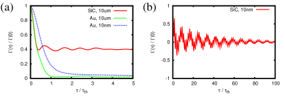
Figure 4: Normalized temporal CFs $\Gamma(\tau)=\langle S_{z}(t)S_{z}(t+\tau)\rangle$ for two SiC and Au halfspaces as function of $\tau$ normalized to $\tau_{\rm th}=\hbar/k_{\rm B}T_{1}\approx 2.5\times 10^{-14}\,{\rm s}$ at $T_{1}=300\,{\rm K}$ and $T_{2}=0\,{\rm K}$ in far-field ($10\,\mu{\rm m}$) and near-field ($d=10\,{\rm nm}$) regime.

Finally, in the general situation where $T_{2}\neq 0\,{\rm K}$, which means that also the thermal sources in the second halfspace need to be taken into account, one can again in a similar way derive the variance $\langle\bigl{(}\Delta S_{z}^{12}\bigr{)}^{2}\rangle\equiv\langle(S_{1,z}-S_{2,z})^{2}\rangle-\langle(S_{1,z}-S_{2,z})\rangle^{2}$ of the heat flux. Furthermore, assuming that the fluctuational sources in the two bodies and also the generated fluctuating fields are uncorrelated, we obtain the general expression

$$\begin{split}\langle\bigl{(}\Delta S_{z}^{12}\bigr{)}^{2}\rangle&=\frac{1}{2}\langle S_{1,z}\rangle^{2}+2\langle E_{1,x}^{2}\rangle\langle H_{1,x}^{2}\rangle\\ &\quad+\frac{1}{2}\langle S_{2,z}\rangle^{2}+2\langle E_{2,x}^{2}\rangle\langle H_{2,x}^{2}\rangle,\end{split}$$ (12)

where $\langle S_{2,z}\rangle$, $\langle E_{2,x}^{2}\rangle$ and $\langle H_{2,x}^{2}\rangle$ take a similar form as $\langle S_{1,z}\rangle$, $\langle E_{1,x}^{2}\rangle$ and $\langle H_{1,x}^{2}\rangle$ but with $T_{2}$ instead of $T_{1}$. Since we assume the absence of correlation between the sources of two different media, we find that the fluctuations are additive. The relative standard deviation is

$$\sigma_{S}^{12}=\frac{\sqrt{\langle\bigl{(}\Delta S_{z}^{12}\bigr{)}^{2}\rangle}}{\langle S_{1,z}\rangle-\langle S_{2,z}\rangle}.$$ (13)

From this expression it becomes clear that this deviation is larger than in the case where $T_{2}=0\,{\rm K}$. As before we can derive the result for two blackbodies in interaction

$$\sigma_{S,BB}^{12}=\frac{\sqrt{\frac{T_{1}^{8}}{T_{2}^{8}}+1}}{\frac{T_{1}^{4}}{T_{2}^{4}}-1}\sqrt{\frac{25}{18}}.$$ (14)

Furthermore, it should be noted that in the limit $\Delta T=T_{1}-T_{2}\rightarrow 0$ the variance in (12) converges to a constant which is, due to the additivity, just twice the value given by eq. (3) corresponding to the deviation for a single semi-infinite medium. That means, although the mean heat flux becomes zero in this limit, the fluctuations of heat flux persist. Therefore, the relative standard deviation $\sigma^{12}_{S}$ can be very large for small temperature differences and even diverges when $\Delta T\rightarrow 0$ as can be nicely seen from expression for the blackbody case where $\sigma^{12}_{S,BB}=\frac{5}{12}\frac{T_{1}}{\Delta T}$ for small $\Delta T$. In Fig. 3 we find at d=10 nm for the heat flux between two SiC (Au) halfspaces a relative standard deviation of $\sigma_{S}^{12}\approx 65$ (81) times the measured heat flux value, which is large and should be measurable in existing near-field heat flux experiments.

We have seen that the heat flux fluctuations are large. But, in order to assess on what extent these fluctuation are measurable it is important to evaluate on which time scale these fluctuations happen. From the blackbody theory it is well known that the CT of thermal field is on the order of $\tau_{\rm th}=\hbar/k_{\rm B}T$ that is about $2.5\times 10^{-14}\,{\rm s}$ at $T=300\,{\rm K}$. This timescale is very similar to the CT we observe in Fig. 4(a) by plotting the temporal CF $\Gamma(\tau)=\langle S_{z}(t)S_{z}(t+\tau)\rangle$ given by SupplM

$$\begin{split}\Gamma(\tau)&=2\langle E_{x}(t)E_{x}(t+\tau)\rangle\langle H_{x}(t)H_{x}(t+\tau)\rangle\\ &\qquad+2\langle E_{x}(t)H_{y}(t+\tau)\rangle^{2}+\langle S_{z}(t)\rangle^{2}\end{split}$$ (15)

of the heat flux between two SiC and Au halfspaces as function of $\tau=t^{\prime}-t$ in the far-field at a distance of $d=10\,\mu{\rm m}$. Although the time scale of $\tau_{\rm th}$ is extremely small, this temporal correlation has been measured in the context of photon bunching Morgan ; TanEtAl2014 . In contrast, if we plot $\Gamma(\tau)$ for a near-field distance of $d=10\,{\rm nm}$ in Fig. 4 (b) we can observe that the timescale on which the heat flux is temporarily correlated is about 50$\times\tau_{\rm th}=1.25\times 10^{-12}\,{\rm s}$ due to the quasi-monochromatic contribution of surface-phonon polariton ShchegrovEtAl2000 . On the other hand, for Au the CT does not change much in the near-fied regime as can be seen in Fig. 4 (a). Hence the timescale of fluctuations of the radiative heat flux in the near field can be on the same order of magnitude as that of relaxations of the phonons in a medium LindeEtAl1980 .

In conclusion, we have introduced a general theory to describe fluctuations of radiative heat flux exchanged between two bodies. We have shown that at subwavelength distances large fluctuations of heat flux can be observed when heat exchanges results from surface polariton coupling. This is in huge contrast to the findings of the zero-point fluctuations of Casimir force Barton1991 ; MessinaPassante2007 . We think that this theory should allow for testing the Crook fluctuation theorem Evans ; Evans2 ; Reid ; Evans3 ; Jarzynski . Hence, by measuring the time evolution of heat flux exchanged between two nanostructures it is in principle possible to calculate the probability to observe an instantaneous negative flux transferred from a cold body to a hot one and to compare this value with the probability of a transfer in the opposite direction. Beyond this fundamental test, this theory can be used to investigate the irreversibility mechanisms associated to thermal photon exchanges Reid ; Evans3 ; Cohen or to explore the performances of nanomachines such as Brownian motors.

S.-A. Biehs acknowledges discussions with Andreas Engel, Achim Kittel (Oldenburg University) and Riccardo Messina (CNRS). P. B.-A. acknowledges discussions with Miguel Rubi (Barcelona University).

References

- (1) E. Akkermans and G. Montambaux, Mesoscopic Physics of Electrons and Photons, Cambridge University Press (2007)
- (2) Y. M. Blanter and M. Büttiker, Physics Reports, 336, 1 (2000).
- (3) C. Beenakker and C. Schönenberger, Phys. Today, 56, 37 (2003).
- (4) M. Planck, The Theory of Heat Radiation (Dover, New York, 1991).
- (5) A. Einstein, Phys. Zeitschr. 10, 185-193, (1909).
- (6) W. Eckhardt, Zeitschrift für Physik B: Condensed Matter, 46 (1982).
- (7) T. Setälä, M. Kaivola, and A. T. Friberg, Phys. Rev. Lett. 88, 123902 (2002).
- (8) P. J. Hesketh, J. N. Zemel, and B. Gebhart, Phys. Rev. B 37(18), 10803-10813 (1988).
- (9) S. M. Rytov, Y. A. Kravtsov, and V. I. Tatarskii, Principles of Statistical Radiophyics (Springer, New York), Vol. 3. (1989).
- (10) D. Polder and M. van Hove, Phys. Rev. B 4, 3303 (1971).
- (11) J. J. Loomis and H. J. Maris, Phys. Rev. B 50, 18517 (1994).
- (12) J. Pendry, J. Phys.: Cond. Mat. 11, 6621 (1999).
- (13) K. Joulain, J.-P. Mulet, F. Marquier, R. Carminati, and J.-J. Greffet, Surf. Sci. Rep. 57, 59 (2005).
- (14) A. I. Volokitin and B. N. J. Persson, Rev. Mod. Phys. 79, 1291 (2007).
- (15) P. Ben-Abdallah and K. Joulain, Phys. Rev. B 82, 121419(R) (2010).
- (16) S.-A. Biehs, E. Rousseau, and J.-J. Greffet, Phys. Rev. Lett. 105, 234301 (2010).
- (17) A. W. Rodriguez, O. Ilic, P. Bermel, I. Celanovic, J. D. Joannopoulos, M. Soljačić, and S. G. Johnson, Phys. Rev. Lett. 107, 114302 (2011).
- (18) A. P. McCauley, M. T. Homer Reid, M. Krüger, and S. G. Johnson, Phys. Rev. B 85, 165104 (2012).
- (19) A. W. Rodriguez, M. T. Homer Reid, and S. G. Johnson, Phys. Rev. B 86, 220302(R) (2012).
- (20) B. Müller, R. Incardone, M. Antezza, T. Emig, and M. Krüger, Phys. Rev. B 95, 085413 (2017).
- (21) G. Bimonte, Phys. Rev. A 80, 042102 (2009).
- (22) M. Krüger, T. Emig, and M. Kardar, Phys. Rev. Lett. 106, 210404 (2011).
- (23) R. Messina and M. Antezza, Europhys. Lett. 95, 61002 (2011).
- (24) M. Krüger, G. Bimonte, T. Emig, and M. Kardar, Phys. Rev. B 86, 115423 (2012).
- (25) R. Messina and M. Antezza, Phys. Rev. A 89, 052104 (2014).
- (26) G. Bimonte, T. Emig, M. Kardar, and M. Krüger, Annu. Rev. Condens. Matter Phys. 8 119 (2017).
- (27) P. Ben-Abdallah, S.-A. Biehs, and K. Joulain, Phys. Rev. Lett. 107, 114301 (2011).
- (28) L. Zhu and S. Fan, Phys. Rev. Lett. 117, 134303 (2016).
- (29) Z. H. Zheng and Y. M. Xuan, Nanoscale and Microscale Thermophysical Engineering 15, 237 (2011).
- (30) R. Messina, M. Antezza, and P. Ben-Abdallah, Phys. Rev. Lett. 109, 244302 (2012).
- (31) P. Ben-Abdallah and S.-A. Biehs, Phys. Rev. Lett. 112, 044301 (2014).
- (32) R. Messina, M. Tschikin, S.-A. Biehs, and P. Ben-Abdallah, Phys. Rev. B 88, 104307 (2013).
- (33) P. Ben-Abdallah, R. Messina, S.-A. Biehs, M. Tschikin, K. Joulain, and C. Henkel, Phys. Rev. Lett. 111, 174301 (2013).
- (34) M. Nikbakht, J. Appl. Phys. 116, 094307 (2014).
- (35) P. Ben-Abdallah, Appl. Phys. Lett. 89, 113117 (2006).
- (36) P. Ben-Abdallah, K. Joulain, J. Drevillon, and C. Le Goff, Phys. Rev. B 77, 075417 (2008).
- (37) M. Nikbakht, Europhys. Lett. 110, 14004 (2015).
- (38) P. Ben-Abdallah, Phys. Rev. Lett. 116, 084301 (2016).
- (39) I. Latella and P. Ben-Abdallah, Phys. Rev. Lett. 118, 173902 (2017).
- (40) C. Hargreaves, Phys. Lett. A 30, 491 (1969).
- (41) A. Kittel, W. Müller-Hirsch, J. Parisi, S.-A. Biehs, D. Reddig, and M. Holthaus, Phys. Rev. Lett. 95, 224301 (2005).
- (42) A. Narayanaswamy, S. Shen, and G. Chen, Phys. Rev. B 78, 115303 (2008).
- (43) L. Hu, A. Narayanaswamy, X. Chen, and G. Chen, Appl. Phys. Lett. 92, 133106 (2008).
- (44) S. Shen, A. Narayanaswamy, and G. Chen, Nano Lett. 9, 2909 (2009).
- (45) E. Rousseau, A. Siria, G. Joudran, S. Volz, F. Comin, J. Chevrier, and J.-J. Greffet, Nat. Photon. 3, 514 (2009).
- (46) R. S. Ottens, V. Quetschke, S. Wise, A. A. Alemi, R. Lundock, G. Mueller, D. H. Reitze, D. B. Tanner, and B. F. Whiting, Phys. Rev. Lett. 107, 014301 (2011).
- (47) T. Kralik, P. Hanzelka, M. Zobac, V. Musilova, T. Fort, and M. Horak, Phys. Rev. Lett. 109, 224302 (2012).
- (48) P. J. van Zwol, L. Ranno, and J. Chevrier, Phys. Rev. Lett. 108, 234301 (2012).
- (49) P. J. van Zwol, S. Thiele, C. Berger, W. A. de Heer, and J. Chevrier, Phys. Rev. Lett. 109, 264301 (2012).
- (50) B. Song, Y. Ganjeh, S. Sadat, D. Thompson, A. Fiorino, V. Fernández-Hurtado, J. Feist, F. J. Garcia-Vidal, J. C. Cuevas, P. Reddy, and E. Meyhofer, Nat. Nanotechnol. 10, 253 (2015).
- (51) K. Kim, B. Song, V. Fernández-Hurtado, W. Lee, W. Jeong, L. Cui, D. Thompson, J. Feist, M. T. H. Reid, F. J. Garcia-Vidal, J. C. Cuevas, E. Meyhofer, and P. Reddy, Nature (London) 528, 387 (2015).
- (52) R. St-Gelais, L. Zhu, S. Fan, and M. Lipson, Nat. Nanotechnol. 11, 515 (2016).
- (53) K. Kloppstech, N. Könne, S.-A. Biehs, A. W. Rodriguez, L. Worbes, D. Hellmann, and A. Kittel, Nat. Commun. 8, 14475 (2017).
- (54) D. J. Evans, E. G. Cohen and G. P. Morriss, Phys. Rev. Lett., 71, 2401 (1993).
- (55) D. J. Evans and D. J. Searles, Adv. Phys., 51, 1529 (2002).
- (56) G. M. Wang, E.M. Sevick, E. Mittag, D.J. Searles and D. J. Evans, Phys. Rev. Lett., 89, 050601 (2002).
- (57) N. Garnier and S. Ciliberto, Phys. Rev. E, 71, 060101 (2005).
- (58) L. Mandel und E. Wolf, Optical Coherence and Quantum Optics, (Cambridge University Press,2008).
- (59) J. R. Zurita-Sánchez, J.-J. Greffet, L. Novotny, Phys. Rev. A 69, 022902 (2004).
- (60) See Supplemental Material at http://link.aps.org/supplemental/ for a brief derivation of the different correlation functions and their symmetry properties, the derivation of the blackbody limit, the quasi-static limit, the temporal correlation function of the Poynting vector, and the Drude-Lorentz and Drude parameters.
- (61) I. A. Dorofeyev and E. A. Vinogradov, Phys. Rep. 75, 504 (2011)
- (62) G. S. Agarwal, Phys. Rev. A 11, 230 (1975).
- (63) W. Eckhardt, Z. Phys. 31, 217 (1978).
- (64) W. Eckhardt, J. Phys. A: MAth. Gen. 12, 1563 (1979).
- (65) Handbook of Optical Constants of Solids, edited by E. Palik (Academic Press, New York, 1998).
- (66) B. L. Morgan and L. Mandel, Phys. Rev. Lett. 16, 1012 (1966).
- (67) P. K. Tan, G. H. Yeo, H. S. Poh, A. H. Chan, and C. Kurtsiefer, Astrophys. J. Lett. 789, L10 (2014).
- (68) A. V. Shchegrov, K. Joulain, R. Carminati, J.-J. Greffet, Phys. Rev. Lett. 85, 1548 (2000).
- (69) D. von der Linde, J. Kuhl, and H. Klingenberg, Phys. Rev. Lett. 44, 1505 (1980).
- (70) G. Barton, J. Phys. A: Math. Gen. 24, 991 (1991).
- (71) R. Messina and R. Passante, Phys. Rev. A 76, 032107 (2007).
- (72) J. C. Reid, E.M. Sevick and D.J. Evans, Europhysics Lett., 72, 726 (2005).
- (73) D. J. Evans, Molecular Physics, 101, 1551 (2003).
- (74) C. Jarzinski, Phys. Rev. Lett., 78, 2690 (1997).
- (75) E.G.D. Cohen, Some recent advances in classical statistical mechanics, P. Garbaczewski and R. Olkiewicz editors, Dynamics of dissipation, Vol. 597, 7, Springer-Verlag, Berlin (2002).