Conserved spin current for the Mott relation

Abstract

The conserved bulk spin current [PRL 96, 076604 (2006)] defined as the time derivative of the spin displacement operator ensures automatically the Onsager relation between the spin Hall effect (SHE) and the inverse SHE. Here we reveal another desirable property of this conserved spin current: the Mott relation exists linking the SHE and its thermal-counterpart – spin Nernst effect (SNE). According to the Mott relation, the SNE is known once the SHE is understood. In the two-dimensional Dirac-Rashba system with smooth scalar disorder-potential, we find a sign change of the spin Nernst conductivity when tuning the chemical potential.

In the rapidly extending fields of spintronics and spin-caloritronics, the spin Hall effect (SHE) Sinova2015 ; Nagaosa2008 and its thermal-counterpart – spin Nernst effect (SNE) Ma2010 ; Dyrdal2016 ; Borge2013 ; SNE2014 ; Tauber2012 ; Meyer2017 ; Sheng2017 ; Kim2017 ; Bose2018 have played important roles. When describing the SHE and SNE in terms of the bulk spin current in the presence of band-structure spin-orbit interaction, there exists the well-known ambiguity about the definition of a transport spin current when the transported spin-component is not conserved. A conserved bulk spin current has been proposed by Shi, Zhang, Xiao and Niu (hereafter we call it the SZXN spin current) Shi2006 ; note-conserve and been studied intensively Zhang2008 ; Wong2008 ; Guo2009 ; Chen2014 ; Freimuth2010 ; Sugimoto2006 ; Mandal2008 ; Gorini2012 . The SZXN spin current operator is described as the time derivative of the spin displacement operator (see below). The so-defined spin current has a natural conjugate force and represents a transport current. The Onsager relation can thus be established automatically between the SHE and inverse SHE of this SZXN spin current Shi2006 ; Zhang2008 ; Gorini2012 . In this Rapid Communication we reveal another desirable property of the SZXN spin current: the Mott relation between the SHE and SNE. The Mott relation Streda1977 can be viewed as a fundamental link between the transport current responses to the electric field and to the temperature gradient in independent-carrier systems with elastic scattering off disorder. According to the Mott relation, the SNE is known once the SHE is understood.

As applications, we show that, in the weak disorder-potential regime, both the SHE and SNE can be finite in the two-dimensional (2D) Dirac-Rashba system with smooth disorder-potential, contrary to the vanishing SHE Sugimoto2006 ; Mandal2008 and SNE in a Rashba 2D electron gas. A sign change of the spin Nernst conductivity is found when tuning the chemical potential.

Generalized Mott relation— The out-of-equilibrium average value of an observable $\hat{O}$ in a single-particle system reads $\delta O=$ Tr$\left\langle\hat{O}^{eq}\left(\delta\hat{\rho}\right)\right\rangle+$ Tr$\left\langle\hat{\rho}^{eq}\delta\hat{O}\right\rangle$ in the linear response regime. Here $\hat{\rho}$ is the single-particle density matrix with $\hat{\rho}^{eq}$ and $\delta\hat{\rho}$ the equilibrium and linear-response components, respectively. $\hat{O}^{eq}$ and $\delta\hat{O}$ have analogous meanings, $\left\langle..\right\rangle$ denotes the disorder averaging. The usual external perturbations driving nonequilibrium steady-states in experiments are electric field $\mathbf{E}$ and temperature gradient $-\mathbf{\nabla}T/T$. For transport effects, the temperature gradient can be equivalently replaced by the gradient $-\mathbf{\nabla}\psi/c^{2}$ of a fictitious gravitational potential $\psi$ introduced by Luttinger (c is the speed of light) Luttinger1964 . The first term of $\delta O$ arises from the density-matrix linear response $\delta\hat{\rho}=\delta^{\mathbf{E}}\hat{\rho}+\delta^{\psi}\hat{\rho}$, whereas the second term comes from the linear response of the observable operator itself with respect to external perturbations $\delta\hat{O}=\delta^{\mathbf{E}}\hat{O}+\delta^{\psi}\hat{O}$. As a result, the linear response of any transport current $\hat{O}$ of a single-electron system with respect to the d.c. uniform $\mathbf{E}$ and $-\mathbf{\nabla}\psi/c^{2}$ reads ($\alpha,\beta=x,y$)

$$\delta O_{\alpha}=L_{\alpha\beta}^{oe}E_{\beta}+L_{\alpha\beta}^{oQ}\left(\frac{-\partial_{\beta}\psi}{c^{2}}\right),$$ (1)

where $L_{\alpha\beta}^{o\xi}=D_{\alpha\beta}^{o\xi}+M_{\alpha\beta}^{o\xi}$ with $D_{\alpha\beta}^{oe}E_{\beta}\equiv$ Tr$\left\langle\hat{O}_{\alpha}^{eq}\delta^{\mathbf{E}}\hat{\rho}\right\rangle$, $D_{\alpha\beta}^{oQ}\left(\frac{-\partial_{\beta}\psi}{c^{2}}\right)\equiv$ Tr$\left\langle\hat{O}_{\alpha}^{eq}\delta^{\psi}\hat{\rho}\right\rangle$, $M_{\alpha\beta}^{oe}E_{\beta}\equiv$ Tr$\left\langle\hat{\rho}^{eq}\delta^{\mathbf{E}}\hat{O}_{\alpha}\right\rangle$ and $M_{\alpha\beta}^{oQ}\left(\frac{-\partial_{\beta}\psi}{c^{2}}\right)\equiv$ Tr$\left\langle\hat{\rho}^{eq}\delta^{\psi}\hat{O}_{\alpha}\right\rangle$. The basic considerations for obtaining $\delta^{\mathbf{E,}\psi}\hat{\rho}$ and $\delta^{\mathbf{E,}\psi}\hat{O}$ can be found in the classical treatment in Ref. Streda1977 , where the electric field enters the total single-carrier Hamiltonian $\hat{H}^{t}$ via the dipole term $-e\mathbf{\hat{r}\cdot E}$. This is the case in the level of the full Hamiltonian Chang2008 ; Xiao2018effective . While in the level of an effective Hamiltonian, the canonical position $\mathbf{\hat{r}}$ may not be the physical one $\mathbf{\hat{r}}^{phy}$ and an anomalous dipole $e\left(\mathbf{\hat{r}}^{phy}-\mathbf{\hat{r}}\right)$ (usually related to effective spin-orbit interaction Sinitsyn2008 ; Culcer2013 ) couples to the electric field Chang2008 . This situation needs separate treatment Culcer2013 ; Xiao2018effective . In the present study we neglect this complexity and take $\mathbf{\hat{r}}^{phy}=\mathbf{\hat{r}}$ approximately even when the transport is calculated in the level of effective Hamiltonians note-appro . Thus the spin-orbit interactions with the external electric field and with the disorder potential Chang2008 ; Xiao2018effective ; Culcer2013 do not appear throughout this Rapid Communication.

$D_{\alpha\beta}^{o\xi}$ is generally given by the Bastin version of $\hat{O}_{\alpha}-\hat{\jmath}_{\beta}^{\xi}$ correlation function Bastin1971 , which can be casted into Bruno2001

$$D_{\alpha\beta}^{o\xi}=D_{\alpha\beta}^{o\xi,I\left(a\right)}+D_{\alpha\beta}^{o\xi,I\left(b\right)}+D_{\alpha\beta}^{o\xi,II}$$ (2)

with

$$D_{\alpha\beta}^{o\xi,I\left(a\right)}=-\frac{\hbar}{2\pi}\int d\epsilon\frac{df^{0}\left(\epsilon\right)}{d\epsilon}\text{Tr}\left\langle\hat{O}_{\alpha}^{eq}\hat{G}^{R}\left(\epsilon\right)\hat{\jmath}_{\beta}^{eq,\xi}\hat{G}^{A}\left(\epsilon\right)\right\rangle,$$

$$D_{\alpha\beta}^{o\xi,I\left(b\right)}=\frac{\hbar}{2\pi}\mathrm{\operatorname{Re}}\int d\epsilon\frac{df^{0}\left(\epsilon\right)}{d\epsilon}\text{Tr}\left\langle\hat{O}_{\alpha}^{eq}\hat{G}^{R}\left(\epsilon\right)\hat{\jmath}_{\beta}^{eq,\xi}\hat{G}^{R}\left(\epsilon\right)\right\rangle,$$

and

$$D_{\alpha\beta}^{o\xi,II} =\frac{\hbar}{2\pi}\operatorname{Re}\int d\epsilon f^{0}\left(\epsilon\right)\text{Tr}\left\langle\hat{O}_{\alpha}^{eq}\hat{G}^{R}\left(\epsilon\right)\hat{\jmath}_{\beta}^{eq,\xi}\frac{d\hat{G}^{R}\left(\epsilon\right)}{d\epsilon}\right.$$

$$\left.-\hat{O}_{\alpha}^{eq}\frac{d\hat{G}^{R}\left(\epsilon\right)}{d\epsilon}\hat{\jmath}_{\beta}^{eq,\xi}\hat{G}^{R}\left(\epsilon\right)\right\rangle.$$

Here $\hat{\jmath}_{\beta}^{eq,\xi}$ stands for the equilibrium electric current ($\xi=e$) and heat current ($\xi=Q$) operators: $\hat{\jmath}_{\beta}^{eq,e}=e\hat{v}_{\beta}$, $\hat{\jmath}_{\beta}^{eq,Q}=\frac{1}{2}\left\{\hat{H}^{eq}-\mu,\hat{v}_{\beta}\right\}$. $\hat{G}^{R/A}\left(\epsilon\right)=\left(\epsilon-\hat{H}^{eq}\pm i0^{+}\right)^{-1}$ with $\hat{H}^{eq}$ the single-particle Hamiltonian at equilibrium, $f^{0}$ is the equilibrium Fermi distribution and $\mu$ is the chemical potential. Now we derive a general relation between $D_{\alpha\beta}^{oQ}$ and $D_{\alpha\beta}^{oe}$. By using $\left(\hat{G}^{R/A}\right)^{2}=-d\hat{G}^{R/A}/d\epsilon$, we get

$$D_{\alpha\beta}^{oQ,I\left(a\right)}=\int d\epsilon\left[-\frac{df^{0}\left(\epsilon\right)}{d\epsilon}\right]\frac{\left(\epsilon-\mu\right)}{e}D_{\alpha\beta}^{oe,I\left(a\right)}\left(T=0,\epsilon\right)+\frac{\hbar}{4\pi}\int d\epsilon\frac{df^{0}\left(\epsilon\right)}{d\epsilon}\text{Tr}\left\langle\hat{O}_{\alpha}^{eq}\hat{v}_{\beta}^{eq}\hat{G}^{A}\left(\epsilon\right)+\hat{v}_{\beta}^{eq}\hat{O}_{\alpha}^{eq}\hat{G}^{R}\left(\epsilon\right)\right\rangle,$$

$$D_{\alpha\beta}^{oQ,I\left(b\right)}=\int d\epsilon\left[-\frac{df^{0}\left(\epsilon\right)}{d\epsilon}\right]\frac{\left(\epsilon-\mu\right)}{e}D_{\alpha\beta}^{oe,I\left(b\right)}\left(T=0,\epsilon\right)-\frac{\hbar}{4\pi}\int d\epsilon\frac{df^{0}\left(\epsilon\right)}{d\epsilon}\text{Tr}\left\langle\frac{1}{2}\left\{\hat{O}_{\alpha}^{eq},\hat{v}_{\beta}^{eq}\right\}\left[\hat{G}^{R}\left(\epsilon\right)+\hat{G}^{A}\left(\epsilon\right)\right]\right\rangle,$$

and

$$D_{\alpha\beta}^{oQ,II}=-\int d\epsilon\left[f^{0}\left(\epsilon\right)+\left(\epsilon-\mu\right)\frac{df^{0}\left(\epsilon\right)}{d\epsilon}\right]\frac{1}{e}D_{\alpha\beta}^{oe,II}\left(T=0,\epsilon\right)+\frac{\hbar}{4\pi}\int d\epsilon\frac{df^{0}\left(\epsilon\right)}{d\epsilon}\text{Tr}\left\langle\frac{1}{2}\left[\hat{O}_{\alpha}^{eq},\hat{v}_{\beta}^{eq}\right]\left[\hat{G}^{R}\left(\epsilon\right)-\hat{G}^{A}\left(\epsilon\right)\right]\right\rangle,$$

then $D_{\alpha\beta}^{oQ}\left(T,\mu\right)=D_{\alpha\beta}^{oQ,I}\left(T,\mu\right)+D_{\alpha\beta}^{oQ,II}\left(T,\mu\right)$ yields the first main result of this paper:

$$D_{\alpha\beta}^{oQ}\left(T,\mu\right)=\int d\epsilon\left[-\frac{df^{0}\left(\epsilon\right)}{d\epsilon}\right]\frac{\left(\epsilon-\mu\right)}{e}D_{\alpha\beta}^{oe}\left(T=0,\epsilon\right)-\frac{1}{e}\int d\epsilon f^{0}\left(\epsilon\right)D_{\alpha\beta}^{oe,II}\left(T=0,\epsilon\right).$$ (3)

On the other hand, utilizing $\left(\hat{G}^{R/A}\right)^{2}=-d\hat{G}^{R/A}/d\epsilon$ and Bruno2001 $i\hbar\hat{G}^{R}\hat{v}_{\beta}^{eq}=\hat{G}^{R}\left[\hat{r}_{\beta},\hat{H}^{eq}\right]=\hat{G}^{R}\left[\left(\hat{G}^{R}\right)^{-1},\hat{r}_{\beta}\right]$, we get

$$D_{\alpha\beta}^{oe,II}=\frac{e}{2}\int d\epsilon\frac{df^{0}\left(\epsilon\right)}{d\epsilon}\text{Tr}\left\langle\left\{\hat{O}_{\alpha}^{eq},\hat{r}_{\beta}\right\}\delta\left(\epsilon-\hat{H}^{eq}\right)\right\rangle+\frac{e}{\pi}\operatorname{Im}\int d\epsilon f^{0}\left(\epsilon\right)\text{Tr}\left\langle\hat{O}_{\alpha}^{eq}\hat{G}^{R}\left(\epsilon\right)\hat{r}_{\beta}\hat{G}^{R}\left(\epsilon\right)\right\rangle.$$

We find that, if the current $\hat{O}_{\alpha}$ is defined in terms of the time derivative of some displacement operators Shi2006 , i.e.,

$$\hat{O}_{\alpha}=\frac{1}{i\hbar}\left[\hat{F}_{\alpha},\hat{H}^{t}\right]\text{ where }\left[\hat{F}_{\alpha},\hat{r}_{\beta}\right]=0,$$ (4)

then $Tr\left\langle\hat{O}_{\alpha}^{eq}\hat{G}^{R}\hat{r}_{\beta}\hat{G}^{R}\right\rangle=\frac{1}{i\hbar}Tr\left\langle\left[\hat{r}_{\beta},\hat{F}_{\alpha}\right]\hat{G}^{R}\right\rangle=0$ and

$$D_{\alpha\beta}^{oe,II}=\frac{e}{2}\int d\epsilon\frac{df^{0}\left(\epsilon\right)}{d\epsilon}\text{Tr}\left\langle\left\{\hat{O}_{\alpha}^{eq},\hat{r}_{\beta}\right\}\delta\left(\epsilon-\hat{H}^{eq}\right)\right\rangle.$$ (5)

For the current $\hat{O}_{\alpha}$ in the form of Eq. (4), one has $\delta^{\mathbf{E}}\hat{O}=0$ and $\delta^{\psi}\hat{O}=\frac{1}{2}\left\{\hat{r}_{\beta}\mathbf{,}\hat{O}^{eq}\right\}\frac{\partial_{\beta}\psi}{c^{2}}$, thus $\delta O_{\alpha}=D_{\alpha\beta}^{oe}E_{\beta}+\left(D_{\alpha\beta}^{oQ}+M_{\alpha\beta}^{oQ}\right)\left(\frac{-\partial_{\beta}\psi}{c^{2}}\right)$, where $M_{\alpha\beta}^{oQ}\left(\frac{-\partial_{\beta}\psi}{c^{2}}\right)\equiv$ Tr$\left\langle\hat{\rho}^{eq}\delta^{\psi}\hat{O}_{\alpha}\right\rangle$ is given by Streda1977

$$M_{\alpha\beta}^{oQ} =-\frac{1}{2}\int d\epsilon f^{0}\left(\epsilon\right)\text{Tr}\left\langle\delta\left(\epsilon-\hat{H}^{eq}\right)\left\{\hat{r}_{\beta},\hat{O}_{\alpha}^{eq}\right\}\right\rangle$$

$$=\frac{1}{e}\int d\epsilon f^{0}\left(\epsilon\right)D_{\alpha\beta}^{oe,II}\left(T=0,\epsilon\right).$$ (6)

Combining Eqs. (5), (6) and (3) yields the generalized Mott relation

$$L_{\alpha\beta}^{oQ}\left(T,\mu\right)=\int d\epsilon\left[-\frac{df^{0}\left(\epsilon\right)}{d\epsilon}\right]\frac{\left(\epsilon-\mu\right)}{e}L_{\alpha\beta}^{oe}\left(T=0,\epsilon\right)$$ (7)

for the current $\hat{O}_{\alpha}$ having the form of Eq. (4). This relation is exactly the same as the well-known generalized Mott relation Streda1977 between $L_{\alpha\beta}^{eQ}$ and $L_{\alpha\beta}^{ee}$. Equations (3) - (7) are the main result of this Rapid Communication. When the distances between the chemical potential and the band edges are much larger than the thermal energy $k_{B}T$, the Sommerfeld expansion is legitimate Xiao2016PRB , yielding the standard Mott relation

$$L_{\alpha\beta}^{oQ}\left(T,\mu\right)/T=\frac{\pi^{2}k_{B}^{2}T}{3e}\frac{\partial L_{\alpha\beta}^{oe}\left(T=0,\epsilon\right)}{\partial\epsilon}|_{\epsilon=\mu},$$ (8)

which relates $L_{\alpha\beta}^{oQ}$ to the energy derivative of $L_{\alpha\beta}^{oe}$ around the chemical potential.

Both the electric current operator $\mathbf{\hat{\jmath}}^{e}=e\frac{1}{i\hbar}\left[\mathbf{\hat{r}},\hat{H}^{t}\right]$ and the SZXN spin current operator $\mathbf{\hat{\jmath}}^{s}=\frac{1}{i\hbar}\left[\mathbf{\hat{r}}\hat{s}_{z},\hat{H}^{t}\right]$ have the form of Eq. (4). Thus the SNE of the SZXN current can be obtained once its SHE is known.

Applications—The intrinsic spin Hall conductivity $\sigma_{yx}^{s,in}$ of the SZXN current can be obtained by standard Kubo formula Shi2006 ; Zhang2008 ; Freimuth2010 . Aside from the intrinsic contribution, there exists disorder-induced contribution to the SHE Sinova2015 ; Nagaosa2008 ; Sugimoto2006 ; Mandal2008 . Among the several mechanisms of the extrinsic contribution, the one arising from the band-off-diagonal elements of the out-of-equilibrium single-carrier density matrix KL1957 ; Luttinger1958 has attracted much recent attention Sinitsyn2008 ; Culcer2017 ; Xiao2017SHE ; Xiao2018scaling . Resorting to the density-matrix transport theory in the weak disorder-potential regime KL1957 ; Culcer2017 ; supp with well-defined multiband structure Xiao2017SOT , this mechanism contributes a spin current in the form off-diagonal

$$\mathbf{j}^{s,ex}=\sum_{l}g_{l}^{\left(-2\right)}\mathbf{j}_{l}^{s,ex}.$$ (9)

Here $g_{l}^{\left(-2\right)}$ is just the conventional out-of-equilibrium distribution function in the Boltzmann transport theory, in the order of $\left\langle V^{2}\right\rangle^{-1}$ with $V$ the disorder potential. $l=\left(\eta,\mathbf{k}\right)$ where $\eta$ is the band index and $\mathbf{k}$ is the momentum. In the case of scalar disorder potential $\left[\mathbf{\hat{r}}\hat{s}_{z},\hat{V}\left(\mathbf{\hat{r}}\right)\right]=0$, we get supp

$$\mathbf{j}_{l}^{s,ex}=\sum_{l^{\prime}}\omega_{l^{\prime}l}^{\left(2\right)}\left(\mathbf{A}_{l^{\prime}}^{s}-\mathbf{A}_{l}^{s}\right)$$ (10)

when $s_{z}^{l}\equiv\langle u_{l}|\hat{s}_{z}|u_{l}\rangle=0$. The expression of $\mathbf{j}_{l}^{s,ex}$ in the case of $s_{z}^{l}\neq 0$ is given in the Supplemental Material supp . Here $\mathbf{A}_{l}^{s}\equiv i\langle u_{l}|\hat{s}_{z}|\partial_{\mathbf{k}}u_{l}\rangle$, $\mathbf{|}l\rangle\equiv|\mathbf{k}\rangle|u_{l}\rangle$ is the eigenstate of the disorder-free equilibrium Hamiltonian $\hat{H}_{0}^{eq}$ with energy $\epsilon_{l}$, and $\omega_{l^{\prime}l}^{\left(2\right)}=\frac{2\pi}{\hbar}\left\langle\left|V_{ll^{\prime}}\right|^{2}\right\rangle\delta\left(\epsilon_{l}-\epsilon_{l^{\prime}}\right)$ is the lowest-Born-order scattering rate. Since $s_{z}^{l}=0$, $\mathbf{A}_{l}^{s}$ is real and remains unchanged under a local U(1) gauge transformation $|u_{l}\rangle\rightarrow e^{i\phi_{l}}|u_{l}\rangle$. The extrinsic contribution Eq. (9) can be independent of both the disorder potential and impurity density, and thus may cancel partly or totally the intrinsic SHE.

In the weak disorder-potential regime other disorder-induced contributions to the SHE Sinitsyn2008 ; Xiao2017SHE ; Xiao2018scaling ; note-extrinsic vanish in the presence of weak scalar scattering when the Berry-curvatures on the Fermi surfaces are zero. This can be appreciated most easily in the limit of smooth disorder-potential varying slowly on the scale of the lattice constant note . Thus the disorder-induced SHE is just given by Eq. (9). This is the case in 2D systems with Rashba spin-orbit interaction, which are the focus in the following model analysis.

We first apply above results to the 2D Rashba model (both Rashba subbands partially occupied, Fig. 1(a)) with smooth scalar-impurity potentials, arriving at vanishing SHE (Supplementary materials supp ) consistent with previous works Sugimoto2006 ; Mandal2008 . According to the generalized Mott relation, the SNE of the SZXN current vanishes.

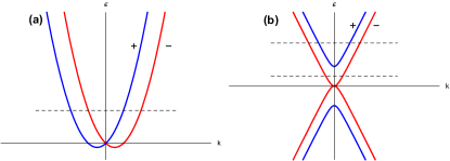
Figure 1: Schematic of the band structures of the 2D Rashba model (a) and 2D Dirac-Rashba model (b).

Now we discuss a model showing nonzero SHE and SNE of the SZXN current. As a minimal model for low-energy electronic states around the Dirac point $K$ in a graphene monolayer subject to $z\rightarrow-z$ asymmetric spin-orbit interaction, the 2D Dirac-Rashba Hamiltonian in the A-B sublattice space reads Rashba2009

$$\hat{H}_{0}^{eq} =v\left[\begin{array}[c]{cc}0&\left(k_{x}-ik_{y}\right)\sigma_{0}\\ \left(k_{x}+ik_{y}\right)\sigma_{0}&0\end{array}\right]$$ (13)

$$+\lambda_{R}\left[\begin{array}[c]{cc}0&\sigma_{y}+i\sigma_{x}\\ \sigma_{y}-i\sigma_{x}&0\end{array}\right].$$ (16)

Here $v=\hbar v_{F}$, $\sigma_{i\text{ }}\left(i=x,y,z\right)$ is the Pauli matrix and $\sigma_{0}$ the unit matrix in the spin space, $\lambda_{R}$ is the Rashba coupling. The four bands of $\hat{H}_{0}^{eq}$ read $\epsilon_{k}^{\eta\zeta}=\eta\left(\sqrt{\lambda_{R}^{2}+\left(vk\right)^{2}}+\zeta\lambda_{R}\right)$. Here $\eta=\pm 1$ denote conduction or valence bands, $\zeta=\pm 1$ denote spin subbands. We only consider the n-doped case (Fig. 1(b)).

For the intrinsic SHE, a lengthy but straightforward calculation leads to the results presented in Table I. In the presence of smooth scalar disorder potential the intervalley scattering is suppressed, thus we obtain

$$\left(\mathbf{j}_{l}^{s,ex}\right)_{y}=-\frac{\hbar}{4}\frac{\hbar v_{F}}{\epsilon_{l}}\sin\xi\frac{1}{\tau_{l}^{tr}}\cos\phi$$ (17)

in Eq. (9), where we use $\left(\mathbf{A}_{\eta\zeta\mathbf{k}}^{s}\right)_{y}=\eta\frac{\hbar}{4}\frac{\hbar v_{F}}{\epsilon_{l}}\sin\xi\cos\phi$ ($s_{z}^{l}=0$ in this model) with $\sin\xi=vk/\sqrt{\lambda_{R}^{2}+\left(vk\right)^{2}}$ and $\tan\phi=k_{y}/k_{x}$. $\tau_{l}^{tr}=1/\sum_{l^{\prime}}\omega_{l^{\prime}l}^{\left(2\right)}\left[1-\cos\left(\phi^{\prime}-\phi\right)\right]$ is the transport time in the case of smooth scalar disorder. The out-of-equilibrium distribution function reads

$$g_{l}^{\left(-2\right)}=\frac{e}{\hbar}\mathbf{E}\cdot\left(-\partial f^{0}/\partial\mathbf{k}\right)\tau_{l}^{tr},$$ (18)

thus Eq. (9) yields the extrinsic SHE listed in Table I. The total spin Hall conductivity $\sigma_{yx}^{s}$ is positive-definite and depends on the Fermi energy, as shown in Table I.

	$\epsilon_{F}>2\lambda_{R}$	$\epsilon_{F}<2\lambda_{R}$
$\sigma_{yx}^{s,in}$	$-\frac{3e}{8\pi}\frac{\epsilon_{F}^{2}-2\lambda_{R}^{2}}{\epsilon_{F}^{2}-\lambda_{R}^{2}}$	$-\frac{e}{16\pi}\frac{2\epsilon_{F}^{2}+\lambda_{R}\epsilon_{F}+2\lambda_{R}^{2}}{\lambda_{R}\left(\epsilon_{F}+\lambda_{R}\right)}$
$\sigma_{yx}^{s,ex}$	$-\frac{e}{8\pi}\frac{\epsilon_{F}^{2}-2\lambda_{R}^{2}}{\epsilon_{F}^{2}-\lambda_{R}^{2}}$	$-\frac{e}{16\pi}\frac{\epsilon_{F}+2\lambda_{R}}{\epsilon_{F}+\lambda_{R}}$
$\sigma_{yx}^{s}=\sigma_{yx}^{s,in}+\sigma_{yx}^{s,ex}$	$-\frac{e}{2\pi}\frac{\epsilon_{F}^{2}-2\lambda_{R}^{2}}{\epsilon_{F}^{2}-\lambda_{R}^{2}}$	$-\frac{e}{8\pi}\frac{\epsilon_{F}^{2}+\lambda_{R}\epsilon_{F}+2\lambda_{R}^{2}}{\lambda_{R}\left(\epsilon_{F}+\lambda_{R}\right)}$

Table 1: The intrinsic ($\sigma_{yx}^{s,in}$) and extrinsic ($\sigma_{yx}^{s,ex}$) spin Hall conductivities in the case of both conduction bands partially occupied ($\epsilon_{F}>2\lambda_{R}$) and of empty inner conduction band ($\epsilon_{F}<2\lambda_{R}$) in the 2D Dirac-Rashba model.

The spin Nernst conductivity $\alpha_{yx}^{s}=L_{yx}^{sQ}\left(T,\mu\right)/T$ is obtained by the Mott relations (7) and (8). In particular, in the case of strong Rashba spin-orbit interaction, the chemical potential may be located in the region $2\lambda_{R}\gg\mu\gg k_{B}T$ ($\epsilon_{k=0}^{++}=2\lambda_{R}$) at low temperatures, then the standard Mott relation (8) applies, yielding

$$\frac{\alpha_{yx}^{s}}{T}=-\frac{\pi k_{B}^{2}}{24\lambda_{R}}\left[1-\frac{3\lambda_{R}^{2}}{\left(\mu+\lambda_{R}\right)^{2}}\right].$$ (19)

This spin Nernst conductivity displays a sign change at $\mu/\lambda_{R}=\sqrt{3}-1$.

Discussion—The SZXN spin current has been proved to obey the basic near-equilibrium transport relations, i.e., the Mott relation established above and the Onsager relation shown previously Shi2006 ; Zhang2008 . On the other hand, for the conventional spin current defined as the anti-commutator of the velocity and spin operators, whether the Mott relation is valid or not (when the transported spin is non-conserved) is still a problem not completely settled in literatures. Here we make some discussions on this issue, because the conventional spin current is frequently used in theoretical formulations of spin transport Sinova2015 , although it is not directly related to the transport of spin in the case of spin non-conservation Halperin2004 . Accordingly, in this case it is expected that the Mott relation as a transport relation does not apply for the conventional spin current. We point out that existing theories indeed do not prove the Mott relation for the conventional spin current. Moreover, a recent work showed the breakdown of the Mott relation for the conventional spin current in a specific model Dyrdal2016 .

The direct application of the Kubo-Luttinger-Streda formalism presented in this study to the thermoelectric response of the conventional spin current does not yield the generalized Mott relation when the transported spin component is not conserved. For the SNE of the conventional spin current, the conventional-spin-current-heat-current correlation function reads supp ($D_{yx}^{s0e}\equiv\sigma_{yx}^{s0}$)

$$D_{yx}^{s0Q}\left(T,\mu\right) =\int d\epsilon\left[-\frac{df^{0}\left(\epsilon\right)}{d\epsilon}\right]\frac{\left(\epsilon-\mu\right)}{e}\sigma_{yx}^{s0}\left(T=0,\epsilon\right)$$

$$-\frac{1}{e}\int d\epsilon f^{0}\left(\epsilon\right)\sigma_{yx}^{s0,II}\left(T=0,\epsilon\right).$$ (20)

However, $M_{yx}^{s0Q}\left(T,\mu\right)+D_{yx}^{s0Q}\left(T,\mu\right)$ cannot yield the Mott relation generally because $M_{yx}^{s0Q}\left(T,\mu\right)$ cannot be expressed as a Fermi sea integral of the so-called “Fermi sea term” Sinova2015 ; note-Fermisea $\sigma_{yx}^{s0,II}\left(T=0,\epsilon\right)$ of the conventional spin Hall conductivity. If one calculated only the spin-current-heat-current correlation function $D_{yx}^{s0Q}$ and neglected concurrently the Fermi sea term $\sigma_{yx}^{s0,II}$ of the spin Hall conductivity, it would be concluded that the Mott relation is valid for the conventional spin current. But this is not correct because generally both of these two contributions are important Grimaldi2006 ; Streda1977 .

In the 2D Rashba model with scalar disorder, $\sigma_{yx}^{s0}=0$ Dimi and thus

$$D_{yx}^{s0Q}=-\frac{1}{e}\int d\epsilon f^{0}\left(\epsilon\right)\sigma_{yx}^{s0,II}\left(T=0,\epsilon\right).$$ (21)

The disorder-free part (dominates $\sigma_{yx}^{s0,II}$ in the weak disorder-potential regime Sinova2015 ) of $\sigma_{yx}^{s0,II}$ is calculated to be $\sigma_{yx}^{s0,II}\left(T=0,\epsilon\right)=\frac{e}{8\pi}\left(\frac{k_{R}}{k_{0}\left(\epsilon\right)}-\frac{k_{0}\left(\epsilon\right)}{k_{R}}\right)\theta\left(-\epsilon\right)$, with $\theta$ the step function and $k_{0}\left(\epsilon\right)=\alpha_{R}^{-1}\sqrt{\epsilon_{R}^{2}+2\epsilon_{R}\epsilon}$. Therefore, in the low-temperature limit $D_{yx}^{s0Q}\left(T\rightarrow 0\right)=-\frac{\epsilon_{R}}{12\pi T}$ is divergent when both Rashba subbands are partially occupied. Recently, Dyrdal et al. Dyrdal2016 directly evaluated the bubble Ma2010 and vertex corrections of $D_{yx}^{s0Q}\left(T,\mu\right)$ in the Rashba model, and obtained the same low-temperature-limit value. They introduced a spin-resolved orbital magnetization by hand and argued that this quantity also contributes a spin current that should be added to the result of the conventional-spin-current-heat-current correlation function Dyrdal2016 . This treatment removes the divergent value of $D_{yx}^{s0Q}$ in the zero-temperature limit in the Rashba model Dyrdal2016 , but yields a SNE which does not follow the generalized Mott relation for the conventional spin current.

In summary, we proved the Mott relation for the spin thermoelectric transport with the SZXN definition of the spin current. First-principle calculations of the intrinsic SHE in terms of the SZXN current has been available in specific materials such as some nonmagnetic hcp metals where the spin-nonconserving part of the spin-orbit interaction could be important Freimuth2010 . Thus the first-principle prediction of the intrinsic SNE according to the Mott relation in these materials can be made.

References

• (1) J. Sinova, S. O. Valenzuela, J. Wunderlich, C. H. Back, and T. Jungwirth, Rev. Mod. Phys. 87, 1213 (2015).
• (2) N. Nagaosa, J. Phys. Soc. Jpn. 77, 031010 (2008).
• (3) Z. Ma, Solid State Commun. 150, 510 (2010).
• (4) K. Tauber, M. Gradhand, D. V. Fedorov, I. Mertig, Phys. Rev. Lett. 109, 026601 (2012).
• (5) J. Borge, C. Gorini, and R. Raimondi, Phys. Rev. B 87, 085309 (2013); S. Tolle, C. Gorini, and U. Eckern, Phys. Rev. B 90, 235117 (2014).
• (6) P. E. Iglesias and J. A. Maytorena, Phys. Rev. B 89, 155432 (2014).
• (7) A. Dyrdał, J. Barnas, and V. K. Dugaev, Phys. Rev. B 94, 035306 (2016); A. Dyrdał, V. K. Dugaev, and J. Barnas, Phys. Rev. B 94, 205302 (2016).
• (8) S. Meyer, Y.-T. Chen, S. Wimmer, M. Althammer, T. Wimmer, R. Schlitz, S. Geprags, H. Huebl, D. Kodderitzsch, H. Ebert, G. E. W. Bauer, R. Gross, and S. T. B. Goennenwein, Nat. Mater. 16, 977 (2017).
• (9) P. Sheng, Y. Sakuraba, Y. Lau, S. Takahashi, S. Mitani, and M. Hayashi, Sci. Adv. 3, e1701503 (2017).
• (10) D. J. Kim, C. Y. Jeon, J. G. Choi, J. W. Lee, S. Surabhi, J. R. Jeong, K. J. Lee, and B. G. Park, Nat. Commun. 8, 1400 (2017).
• (11) A. Bose, S. Bhuktare, H. Singh, S. Dutta, V. G. Achanta, and A. A. Tulapurkar, Appl. Phys. Lett. 112, 162401 (2018).
• (12) J. Shi, P. Zhang, D. Xiao, and Q. Niu, Phys. Rev. Lett. 96, 076604 (2006).
• (13) The SZXN spin current is conserved in the sense that the field-generated spin torque does not appear in the spin continuity equation, and the latter still includes a spin relaxation term.
• (14) P. Zhang, Z. Wang, J. Shi, D. Xiao, and Q. Niu, Phys. Rev. B 77, 075304 (2008).
• (15) A. Wong, J. A. Maytorena, C. Lopez-Bastidas, and F. Mireles, Phys. Rev. B 77, 035304 (2008); A. Wong and F. Mireles, Phys. Rev. B 81, 085304 (2010).
• (16) T.-W. Chen and G. Y. Guo, Phys. Rev. B 79, 125301 (2009).
• (17) F. Freimuth, S. Blugel, and Y. Mokrousov, Phys. Rev. Lett. 105, 246602 (2010).
• (18) C. Gorini, R. Raimondi, and P. Schwab, Phys. Rev. Lett. 109, 246604 (2012). This paper also explained that the SZXN spin current is not the unique way to define the Onsager reciprocal relation.
• (19) T.-W. Chen, J.-H. Li, and C.-D. Hu, Phys. Rev. B 90, 195202 (2014).
• (20) N. Sugimoto, S. Onoda, S. Murakami, and N. Nagaosa, Phys. Rev. B 73, 113305 (2006).
• (21) S. S. Mandal and A. Sensharma, Phys. Rev. B 78, 205313 (2008).
• (22) L. Smrčka and P. Středa, J. Phys. C 10, 2153 (1977).
• (23) J. M. Luttinger, Phys. Rev. 135, A1505 (1964).
• (24) P. Nozieres and C. Lewiner, J. Phys. (Paris) 34, 901 (1973); M. C. Chang, Q. Niu, J. Phys.: Condens. Matter 20 193202 (2008).
• (25) C. Xiao, B. Xiong, and F. Xue, arXiv: 1803.08164
• (26) X. Bi, P. He, E. M. Hankiewicz, R. Winkler, G. Vignale, and D. Culcer, Phys. Rev. B 88, 035316 (2013).
• (27) N. A. Sinitsyn, J. Phys.: Condens. Matter 20, 023201 (2008).
• (28) This approximation is acceptable when the spin Hall current due to the band-structure (bands of the effective Hamiltonian) spin-orbit interaction is finite. This is because, compared to the band-structure spin-orbit interaction, the effects of the effective spin-orbit interaction (with the external electric field and impurity potential) are usually weak due to the weakness of its strength (see, e.g., Ref. Sinitsyn2008 ). In the Rashba 2D electron gas, the spin Hall current due to the Rashba spin-orbit interaction is zero in the weak disorder-potential regime supp , thus the effective spin-orbit interaction should be considered. Therefore, the application of our results to the 2D Rashba electron gas has mainly methodological or pedagogical meaning, aiming at showing the consistency of our results for SHE and previous works.
• (29) A. Bastin, C. Lewiner, O. Betbeder-Matibet, and P. Nozieres, J. Phys. Chem. Solids 32, 1811 (1971).
• (30) A. Crepieux and P. Bruno, Phys. Rev. B 64, 014416 (2001).
• (31) C. Xiao, D. Li, and Z. Ma, Phys. Rev. B 93, 075150 (2016).
• (32) W. Kohn and J. M. Luttinger, Phys. Rev. 108, 590 (1957).
• (33) J. M. Luttinger, Phys. Rev. 112, 739 (1958).
• (34) D. Culcer, A. Sekine, and A. H. MacDonald, Phys. Rev. B 96, 035106 (2017).
• (35) C. Xiao, Front. Phys. 13, 137202 (2018).
• (36) C. Xiao, B. Xiong, and F. Xue, arXiv: 1802.09716
• (37) Supplementary materials
• (38) C. Xiao and Q. Niu, Phys. Rev. B 96, 035423 (2017).
• (39) In the density-matrix transport theory designed in the weak disorder-potential regime, the off-diagonal elements of the out-of-equilibrium single-particle density matrix can be expressed by the diagonal ones, as detailed in Refs. Luttinger1958 ; Xiao2018scaling . Thus in Eq. (9) one only has the diagonal elements $g_{l}^{\left(-2\right)}$.
• (40) These contributions come from the electric-field working during the scattering, the scattering off pairs of impurities and the skew scattering due to non-Gaussian third-order disorder correlation, see Refs. Sinitsyn2008 ; Xiao2017SHE .
• (41) See Eq. (13) in N. A. Sinitsyn, Q. Niu, J. Sinova, and K. Nomura, Rev. B 72, 045346 (2005), Eq. (3.14) in Ref. Luttinger1958 and the expressions given in Appendix B of Ref. Xiao2018scaling .
• (42) E. I. Rashba, Phys. Rev. B 79, 161409(R) (2009); A. Dyrdał, V. K. Dugaev, and J. Barnas, Phys. Rev. B 80, 155444 (2009).
• (43) E. G. Mishchenko, A. V. Shytov, and B. I. Halperin, Phys. Rev. Lett. 93, 226602 (2004).
• (44) $\sigma_{yx}^{s0,II}$ is called Fermi sea term because its formal expression includes the contribution from states below the Fermi surface, see Ref. Sinova2015 .
• (45) C. Grimaldi, E. Cappelluti, and F. Marsiglio, Phys. Rev. B 73, 081303(R) (2006).
• (46) O. V. Dimitrova, Phys. Rev. B 71, 245327 (2005).