Fine structure of the cross sections of $e^{+}e^{-}$ annihilation near the thresholds of $p\bar{p}$ and $n\bar{n}$ production

Abstract

The energy dependence of the cross sections of $p\bar{p}$, $n\bar{n}$, and meson production in $e^{+}e^{-}$ annihilation in the vicinity of the $p\bar{p}$ and $n\bar{n}$ thresholds is studied. The proton-neutron mass difference and the $p\bar{p}$ Coulomb interaction are taken into account. The values of the cross sections are very sensitive to the parameters of the optical potential. It is shown that the commonly accepted factorization approach for the account of the Coulomb interaction does not work well enough in the vicinity of the threshold due to the finite size of the optical potential well.

I Introduction

In a set of experiments it has been shown that the cross sections of $e^{+}e^{-}$ annihilation into $p\bar{p}$ (Aubert2006, ; Lees2013, ; Lees2013a, ; Akhmetshin2016, ), $n\bar{n}$ (Achasov2014, ) and mesons (Aubert2006a, ; Aubert2007b, ; Akhmetshin2013, ; Lukin2015, ) near the thresholds of $N\bar{N}$ production reveal the unusual behavior. Namely, in this region the cross sections strongly depend on the energy. Similar effects have also been observed in the decays $J/\psi(\psi^{\prime})\to p\bar{p}\pi^{0}(\eta)$ (Bai2003, ; Ablikim2009, ; Bai2001, ) and $J/\psi(\psi^{\prime})\to p\bar{p}\omega(\gamma)$ (Bai2003, ; Alexander2010, ; Ablikim2012, ; Ablikim2008, ; Ablikim2013b, ).

At present, this interesting property is widely discussed by many authors  (dmitriev2007final, ; dmitriev2014isoscalar, ; Haidenbauer2014, ; Haidenbauer2015, ; Kang2015, ; Dmitriev2016, ; Dmitriev2016a, ; Milstein2017, ). A natural explanation of this phenomenon is the nucleon-antinucleon final-state interaction. In the low-energy region this interaction is usually taken into account by means of the optical potentials (el-bennich2009paris, ; zhou2012energy, ; Kang2014, ). The potentials have been proposed to fit the nucleon-antinucleon scattering data, which include the elastic, charge-exchange, and annihilation cross sections, as well as some single-spin observables. For $e^{+}e^{-}$ annihilation, the use of all optical potentials leads to a qualitative agreement of the predictions for the cross sections with the experimental data. However, these data are obtained in the region where the Coulomb interaction and the proton-neutron mass difference are irrelevant.

At present, the CMD-3 detector at the VEPP-2000 collider collects the data on the production of $p\bar{p}$ pair in $e^{+}e^{-}$ annihilation at energies only slightly higher than the pair production threshold Sol2017 . In particular, the energy resolution of this facility allows one to obtain the data between the thresholds of $p\bar{p}$ and $n\bar{n}$ pair production. In this energy region the account for the isospin symmetry violation, following from the proton-neutron mass difference and the $p\bar{p}$ Coulomb interaction, becomes important. The detailed theoretical investigation of the cross sections in the energy region around a few MeV from the thresholds and subsequent comparison of the predictions with the experimental results will allow one to improve the parameters of the optical potentials. Besides, such investigation will elucidate the influence of various effects on the strong energy dependence of the cross sections near the thresholds. This is the main goal of our paper.

II Approach to the calculation of the cross sections

In our previous papers (dmitriev2007final, ; Dmitriev2016, ) we have calculated the cross sections of the processes $e^{+}e^{-}\to p\bar{p},\,n\bar{n}$ and $e^{+}e^{-}\to\mathrm{mesons}$ near the threshold, neglecting the electromagnetic $p\bar{p}$ interaction and the proton-neutron mass difference. The strong energy dependence of the cross section $e^{+}e^{-}\to\mathrm{mesons}$ near the $N\bar{N}$ threshold is related to the production of a virtual $N\bar{N}$ pair with its subsequent annihilation. The interaction of real nucleon and antinucleon or virtual nucleon and antinucleon has been taken into account by means of the optical potentials. In the approach of Refs. (dmitriev2007final, ; Dmitriev2016, ) it was possible to calculate separately the amplitudes corresponding to the states of $N\bar{N}$ pair with the isospin $I=0$ and $I=1$. In this section we generalize that approach to the case of isospin symmetry violation. In this case it is convenient to use the physical particle basis, $p\bar{p}$ and $n\bar{n}$, instead of the isospin basis, $\left(p\bar{p}+n\bar{n}\right)/\sqrt{2}$ for $I=0$ and $\left(p\bar{p}-n\bar{n}\right)/\sqrt{2}$ for $I=1$.

The coupled-channels radial Schrödinger equation for the ${}^{3}S_{1}-^{3}D_{1}$ states reads

$$\left[p_{r}^{2}+\mu\mathcal{V}-\mathcal{K}^{2}\right]\Psi=0\,,\qquad\Psi^{T}=\left(u^{p},w^{p},u^{n},w^{n}\right),$$

$$\mathcal{K}^{2}=\begin{pmatrix}k_{p}^{2}\mathbb{I}&0\\ 0&k_{n}^{2}\mathbb{I}\end{pmatrix},\qquad\mathbb{I}=\begin{pmatrix}1&0\\ 0&1\end{pmatrix},$$

$$\mu=\frac{1}{2}\left(m_{p}+m_{n}\right),\qquad k_{p}^{2}=\mu E\,,\qquad k_{n}^{2}=\mu(E-2\Delta)\,,\qquad\Delta=m_{n}-m_{p}\,,$$ (1)

where $\Psi^{T}$ denotes a transposition of $\Psi$, $(-p_{r}^{2})$ is the radial part of the Laplace operator, $u^{p}(r)$, $w^{p}(r)$ and $u^{n}(r)$, $w^{n}(r)$ are the radial wave functions of a proton-antiproton or neutron-antineutron pair with the orbital angular momenta $L=0$ and $L=2$, respectively, $m_{p}$ and $m_{n}$ are the proton and neutron masses, $E$ is the energy of a system counted from the $p\bar{p}$ threshold, $\hbar=c=1$. In Eq. (1), $\mathcal{V}$ is the matrix $4\times 4$ which accounts for the $p\bar{p}$ interaction and $n\bar{n}$ interaction as well as a transition $p\bar{p}\leftrightarrow n\bar{n}$. This matrix can be written in a block form as

$$\mathcal{V}=\begin{pmatrix}\mathcal{V}^{pp}&\mathcal{V}^{pn}\\ \mathcal{V}^{pn}&\mathcal{V}^{nn}\end{pmatrix},$$ (2)

where the matrix elements read

$${\cal V}^{pp}=\frac{1}{2}({\cal U}^{1}+{\cal U}^{0})-\frac{\alpha}{r}\mathbb{I}+{\cal U}_{cf}\,,\qquad{\cal V}^{nn}=\frac{1}{2}({\cal U}^{1}+{\cal U}^{0})+{\cal U}_{cf}\,,$$

$${\cal V}^{pn}=\frac{1}{2}({\cal U}^{0}-{\cal U}^{1})\,,\qquad{\cal U}_{cf}=\frac{6}{\mu r^{2}}\begin{pmatrix}0&0\\ 0&1\end{pmatrix}\,,\qquad{\cal U}^{I}=\begin{pmatrix}V_{S}^{I}&-2\sqrt{2}\,V_{T}^{I}\\ -2\sqrt{2}\,V_{T}^{I}&\;V_{D}^{I}-2V_{T}^{I}\end{pmatrix},$$ (3)

where $\alpha$ is the fine-structure constant, $V_{S}^{I}(r)$, $V_{D}^{I}(r)$, and $V_{T}^{I}(r)$ are the terms in the potential $V^{I}$ of the strong $N\bar{N}$ interaction, corresponding to the isospin $I$,

$$V^{I}=V_{S}^{I}(r)\delta_{L0}+V_{D}^{I}(r)\delta_{L2}+V_{T}^{I}(r)\left[6\left(\bm{S}\cdot\bm{n}\right)^{2}-4\right].$$ (4)

Here $\bm{S}$ is the spin operator of the produced pair ($S=1$) and $\bm{n}=\bm{r}/r$.

The asymptotic forms of four independent regular solutions of Eq. (1) (they have no singularities at $r=0$) at large distances are

$$\Psi_{1R}^{T}(r)=\frac{1}{2i}\left(S_{11}\chi_{p0}^{+}-\chi_{p0}^{-},\,S_{12}\chi_{p2}^{+},\,S_{13}\chi_{n0}^{+},\,S_{14}\chi_{n2}^{+}\right),$$

$$\Psi_{2R}^{T}(r)=\frac{1}{2i}\left(S_{21}\chi_{p0}^{+},\,S_{22}\chi_{p2}^{+}-\chi_{p2}^{-},\,S_{23}\chi_{n0}^{+},\,S_{24}\chi_{n2}^{+}\right),$$

$$\Psi_{3R}^{T}(r)=\frac{1}{2i}\left(S_{31}\chi_{p0}^{+},\,S_{32}\chi_{p2}^{+},\,S_{33}\chi_{n0}^{+}-\chi_{n0}^{-},\,S_{34}\chi_{n2}^{+}\right),$$

$$\Psi_{4R}^{T}(r)=\frac{1}{2i}\left(S_{41}\chi_{p0}^{+},\,S_{42}\chi_{p2}^{+},\,S_{43}\chi_{n0}^{+},\,S_{44}\chi_{n2}^{+}-\chi_{n2}^{-}\right).$$ (5)

Here $S_{ij}$ are some functions of the energy and

$$\chi_{pl}^{\pm}=\frac{1}{k_{p}r}\exp\left[\vphantom{\bigl{(}\bigr{)}}\pm i\left(k_{p}r-l\pi/2+\eta\ln(2k_{p}r)+\sigma_{l}\right)\right],$$

$$\chi_{nl}^{\pm}=\frac{1}{k_{n}r}\exp\left[\vphantom{\bigl{(}\bigr{)}}\pm i\left(k_{n}r-l\pi/2\right)\right],$$

$$\sigma_{l}=\frac{i}{2}\ln\frac{\Gamma\left(1+l+i\eta\right)}{\Gamma\left(1+l-i\eta\right)}\,,\qquad\eta=\frac{m_{p}\alpha}{2k_{p}}\,,$$ (6)

where $\Gamma(x)$ is the Euler $\Gamma$ function.

At small distances a virtual photon can produce a virtual $p\bar{p}$ pair with the amplitude $g_{p}$ and a virtual $n\bar{n}$ pair with the amplitude $g_{n}$. Then, as a result of $N\bar{N}$ interaction, each of these virtual pairs can produce either a real $p\bar{p}$ or a real $n\bar{n}$ pair in the final state. Therefore, in the non-relativistic approximation the amplitudes of $N\bar{N}$ pair production in $e^{+}e^{-}$ annihilation can be written in units $\pi\alpha/\mu^{2}$ as follows (cf. (Dmitriev2016, )):

$$T_{\lambda^{\prime}\lambda}^{p\bar{p}}=\sqrt{2}\left[g_{p}u_{1R}^{p}(0)+g_{n}u_{1R}^{n}(0)\right](\bm{e}_{\lambda^{\prime}}\cdot\bm{\epsilon}_{\lambda}^{*})\\ +\left[g_{p}u_{2R}^{p}(0)+g_{n}u_{2R}^{n}(0)\right]\left[(\bm{e}_{\lambda^{\prime}}\cdot\bm{\epsilon}_{\lambda}^{*})-3(\hat{\bm{k}}\cdot\bm{e}_{\lambda^{\prime}})(\hat{\bm{k}}\cdot\bm{\epsilon}_{\lambda}^{*})\right],\\ T_{\lambda^{\prime}\lambda}^{n\bar{n}}=\sqrt{2}\left[g_{p}u_{3R}^{p}(0)+g_{n}u_{3R}^{n}(0)\right](\bm{e}_{\lambda^{\prime}}\cdot\bm{\epsilon}_{\lambda}^{*})\\ +\left[g_{p}u_{4R}^{p}(0)+g_{n}u_{4R}^{n}(0)\right]\left[(\bm{e}_{\lambda^{\prime}}\cdot\bm{\epsilon}_{\lambda}^{*})-3(\hat{\bm{k}}\cdot\bm{e}_{\lambda^{\prime}})(\hat{\bm{k}}\cdot\bm{\epsilon}_{\lambda}^{*})\right],$$ (7)

where $\bm{e}_{\lambda^{\prime}}$ is a virtual photon polarization vector, corresponding to the spin projection $J_{z}=\lambda^{\prime}=\pm 1$, $\bm{\epsilon}_{\lambda}$ is the spin-1 function of $N\bar{N}$ pair, $\lambda=\pm 1,\,0$ is the spin projection on the nucleon momentum $\bm{k}$, and $\hat{\bm{k}}=\bm{k}/k$. In Eq. (7) the quantities $u_{iR}^{p}(r)$ and $u_{iR}^{n}(r)$ denote the first and third components of the regular solutions $\Psi_{iR}(r)$ having the asymptotic forms (5). In the vicinity of the thresholds, the amplitudes $g_{p}$ and $g_{n}$ can be considered as the energy independent parameters. Their explicit values are determined by the comparison of predictions with the experimental data.

Above the threshold, in the non-relativistic approximation the standard formula for the differential cross section of $N\bar{N}$ pair production in $e^{+}e^{-}$ annihilation reads

$$\frac{d\sigma^{N}}{d\Omega}=\frac{k_{N}\alpha^{2}}{16\mu^{3}}\left[\left|G_{M}^{N}(E)\right|^{2}\left(1+\cos^{2}\theta\right)+\left|G_{E}^{N}(E)\right|^{2}\sin^{2}\theta\right].$$ (8)

Here $\theta$ is the angle between the electron (positron) momentum and the momentum of the final particle. Using the amplitudes (7) we find the proton and neutron Sachs form factors:

$$G_{M}^{p}=g_{p}u_{1R}^{p}(0)+g_{n}u_{1R}^{n}(0)+\frac{1}{\sqrt{2}}\left[\vphantom{\Bigl{(}\Bigr{)}}g_{p}u_{2R}^{p}(0)+g_{n}u_{2R}^{n}(0)\right],$$

$$G_{E}^{p}=g_{p}u_{1R}^{p}(0)+g_{n}u_{1R}^{n}(0)-\vphantom{\frac{1}{\sqrt{2}}}\sqrt{2}\left[\vphantom{\Bigl{(}\Bigr{)}}g_{p}u_{2R}^{p}(0)+g_{n}u_{2R}^{n}(0)\right],$$

$$G_{M}^{n}=g_{p}u_{3R}^{p}(0)+g_{n}u_{3R}^{n}(0)+\frac{1}{\sqrt{2}}\left[\vphantom{\Bigl{(}\Bigr{)}}g_{p}u_{4R}^{p}(0)+g_{n}u_{4R}^{n}(0)\right],$$

$$G_{E}^{n}=g_{p}u_{3R}^{p}(0)+g_{n}u_{3R}^{n}(0)-\vphantom{\frac{1}{\sqrt{2}}}\sqrt{2}\left[\vphantom{\Bigl{(}\Bigr{)}}g_{p}u_{4R}^{p}(0)+g_{n}u_{4R}^{n}(0)\right].$$ (9)

The integrated cross sections of the nucleon-antinucleon pair production have the form

$$\sigma_{\mathrm{el}}^{p}=\frac{\pi k_{p}\alpha^{2}}{4\mu^{3}}\left[\left|g_{p}u_{1R}^{p}(0)+g_{n}u_{1R}^{n}(0)\right|^{2}+\left|g_{p}u_{2R}^{p}(0)+g_{n}u_{2R}^{n}(0)\right|^{2}\right],$$

$$\sigma_{\mathrm{el}}^{n}=\frac{\pi k_{n}\alpha^{2}}{4\mu^{3}}\left[\left|g_{p}u_{3R}^{p}(0)+g_{n}u_{3R}^{n}(0)\right|^{2}+\left|g_{p}u_{4R}^{p}(0)+g_{n}u_{4R}^{n}(0)\right|^{2}\right].$$ (10)

The label “el” indicates that the process is elastic, i.e., a virtual $N\bar{N}$ pair transfers to a real pair in a final state. There is also an inelastic process when a virtual $N\bar{N}$ pair transfers into mesons in a final state, we denote the corresponding cross section as $\sigma_{\mathrm{in}}$. The total cross section, $\sigma_{\mathrm{tot}}$, is

$$\sigma_{\mathrm{tot}}=\sigma_{\mathrm{el}}^{p}+\sigma_{\mathrm{el}}^{n}+\sigma_{\mathrm{in}}\,.$$ (11)

The total cross section may be expressed via the Green’s function ${\cal D}(r,\,r^{\prime}|E)$ of the equation (1), cf. (Dmitriev2016, ):

$$\sigma_{\mathrm{tot}}=\frac{\pi\alpha^{2}}{4\mu^{3}}\mathop{Im}\left[\mathcal{G}^{\dagger}{\cal D}\left(0,\,0|E\right)\mathcal{G}\right], \mathcal{G}^{T}=\left(g_{p},\,0,\,g_{n},\,0\right),$$ (12)

where the function ${\cal D}(r,\,r^{\prime}|E)$ satisfies the equation

$$\left[p_{r}^{2}+\mu\mathcal{V}-\mathcal{K}^{2}\right]{\cal D}\left(r,\,r^{\prime}|E\right)=\frac{1}{rr^{\prime}}\delta\left(r-r^{\prime}\right)\,.$$ (13)

The solution of Eq. (13) at $r^{\prime}=0$ can be written as follows

$${\cal D}\left(r,\,0|E\right)=k_{p}\left[\Psi_{1N}(r)\Psi_{1R}^{T}(0)+\Psi_{2N}(r)\Psi_{2R}^{T}(0)\right]+k_{n}\left[\Psi_{3N}(r)\Psi_{3R}^{T}(0)+\Psi_{4N}(r)\Psi_{4R}^{T}(0)\right],$$ (14)

Non-regular solutions of the Schrödinger equation (1) are defined by their asymptotic behavior at large distances:

$$u_{1N}^{p}(r)=\chi_{p0}^{+}\,, w_{2N}^{p}(r)=\chi_{p2}^{+}\,, u_{3N}^{n}(r)=\chi_{n0}^{+}\,, w_{4N}^{n}(r)=\chi_{n2}^{+}\,.$$ (15)

All other elements $\psi_{i}$ of the non-regular solutions satisfy the relation

$$\lim_{r\to\infty}r\psi_{i}(r)=0\,.$$

The energy dependence of the cross sections is determined by the parameters of the optical potential. We have found these parameters using the experimental data available. The detailed description of our optical potential and the explicit values of the potential parameters are presented in the Appendix. The results of the calculations, based on our optical potential, are discussed in the next section.

III Results and Discussion

In the present paper we use the same parametrization of the nucleon-antinucleon optical potential of the strong interaction in ${}^{3}S_{1}$ and ${}^{3}D_{1}$ partial waves as in Refs. (Dmitriev2016, ; Dmitriev2016a, ). Namely, each term $V_{S,D,T}^{I}$ in Eq. (4) is a sum of the potential wells and the pion exchange contribution. Besides, these potential wells consist of the real and imaginary parts. The account for the Coulomb potential and the proton-neutron mass difference changes the low-energy behavior of the model. Therefore, the parameters of the model have to be refitted in order to obtain a better description of the experimental data at low energies. These data are the cross sections of nucleon-antinucleon scattering, the cross sections of nucleon-antinucleon pair production in $e^{+}e^{-}$ annihilation, the ratio of the electromagnetic form factors of the proton, and the $p\bar{p}$ invariant mass spectra in the decays $J/\psi\to p\bar{p}\pi^{0}(\eta)$.

In order to understand the influence of the Coulomb potential and the proton-neutron mass difference, we compare our predictions with the results obtained at $\Delta=0$ and with the Coulomb potential taken into account and without account for both isospin-violating effects. The results of our calculations for $e^{+}e^{-}\to p\bar{p}$ and $e^{+}e^{-}\to n\bar{n}$ are shown in Fig. 1. For the process $e^{+}e^{-}\to p\bar{p}$, we conclude that the influence of the Coulomb interaction on the cross section is noticeable only in the energy region of about $2\,\mathrm{MeV}$ above the threshold. The main effect of the Coulomb interaction is the non-zero cross section at $E=0$ (the so-called Sommerfeld-Gamow-Sakharov effect). The influence of the proton-neutron mass difference on the cross section of $p\bar{p}$ production is also small.

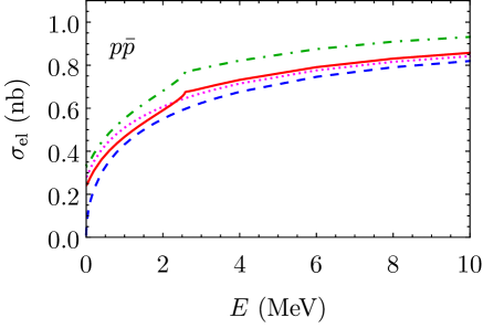
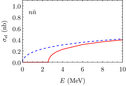
Figure 1: The elastic cross sections of $p\bar{p}$ (left) and $n\bar{n}$ (right) production as a function of the energy $E$ of a pair. Solid curves are the exact results, dashed curves are obtained at $\Delta=0$ and without account for the Coulomb potential, dotted curve in the left picture is obtained at $\Delta=0$ and with account for the Coulomb potential, dash-dotted curve in the left picture corresponds to the approximation (16).

We emphasize the following statement. It is commonly accepted that $\sigma_{\mathrm{el}}$ for the process $e^{+}e^{-}\to p\bar{p}$ can be written as

$$\sigma_{\mathrm{el}}=C\sigma_{\mathrm{el}}^{(0)}\,,\quad C=\frac{2\pi\eta}{1-e^{-2\pi\eta}}\,,$$ (16)

where $\sigma_{\mathrm{el}}^{(0)}$ is the cross section calculated without account for the Coulomb potential and $C$ is the Sommerfeld-Gamow-Sakharov factor. However, it is seen from Fig. 1 that this formula does not work well enough. This circumstance is related to the finite size of the potential wells. Very recently, similar conclusion has been made in Ref. (Voloshin2018, ) at the discussion of the charged-to-neutral meson yield ratio in the decays of $\psi(3770)$ and $\Upsilon(4S)$.

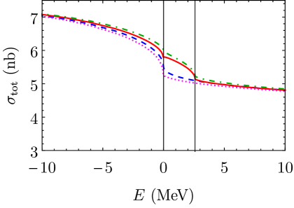
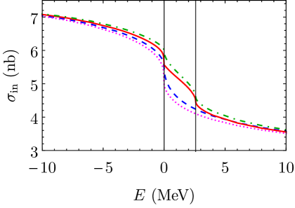
Figure 2: The total cross section $\sigma_{\mathrm{tot}}$ (left) and inelastic cross section $\sigma_{\mathrm{in}}$ (right) as a function of the energy $E$. Solid curves correspond to the exact results, dashed curves are the results, obtained at $\Delta=0$ and without account for the Coulomb interaction, dotted curves are obtained at $\Delta=0$ and with account for the Coulomb potential, and dash-dotted curves are obtained at $\Delta\neq 0$ and without account for the Coulomb potential. Vertical lines show the thresholds of $p\bar{p}$ and $n\bar{n}$ pair production.

Note that an influence of the Coulomb effect on the $n\bar{n}$ pair production cross section is negligible, and we did not show the curves in the right picture of Fig. 1 obtained without account for the Coulomb field. As it should be, the account for non-zero $\Delta$ near the threshold is important for the cross section of $n\bar{n}$ pair production.

In Fig. 2 we show the results for $\sigma_{\mathrm{tot}}$ (left picture) and $\sigma_{\mathrm{in}}$ (right picture) obtained in the different approximations. Solid curves correspond to the exact results, dashed curves are the results obtained at $\Delta=0$ and without account for the Coulomb potential, dotted curves are obtained at $\Delta=0$ and with account for the Coulomb potential, and dash-dotted curves are obtained at $\Delta\neq 0$ and without account for the Coulomb potential. It is seen that the total cross section $\sigma_{\mathrm{tot}}$ is a continuous function of $E$, while $\sigma_{\mathrm{in}}$ has a discontinuity at the proton threshold because of the Coulomb interaction (i.e., because of the Sommerfeld-Gamow-Sakharov effect). The non-zero $\Delta$ results in the essential modification of the cross sections in the vicinity of the thresholds. In the very narrow region below $p\bar{p}$ production threshold, $-15\,\mathrm{keV}<E<0$, the energy dependence of the cross sections is not smooth because of the Coulomb bound states essentially modified by the strong interaction. However, this very narrow region is almost impossible to study experimentally, and we do not show the cross sections in this region in a separate figure.

IV Conclusion

In this paper we have investigated in detail the energy dependence of the cross sections of $p\bar{p}$, $n\bar{n}$, and meson production in $e^{+}e^{-}$ annihilation in the vicinity of the $p\bar{p}$ and $n\bar{n}$ thresholds. The isospin-violating effects, the proton-neutron mass difference and the Coulomb interaction, have been taken into account. The account for both effects turned out to be important in this energy region. Besides, the energy dependence of the cross sections is very sensitive to the parameters of the optical potential. Therefore, the detailed experimental investigation of the cross sections under discussion is very important for refinement of these parameters. We have also found that the commonly accepted factorization approach for the account of the Coulomb potential does not work well enough in the vicinity of the threshold due to the finite size of the optical potential well.

Appendix

In the appendix we describe the optical potential used in our calculations. The optical potential $V$ is expressed via the potentials $\widetilde{U}^{I}$ as follows

$$V(r)=\widetilde{U}^{0}+\left(\bm{\tau}_{1}\cdot\bm{\tau}_{2}\right)\widetilde{U}^{1},$$ (17)

where $\bm{\tau}_{1,2}$ are the isospin Pauli matrices. Therefore, the terms $V_{S,D,T}^{I}$ in Eq. (4) are

$$V_{i}^{1}(r)=\widetilde{U}_{i}^{0}(r)+\widetilde{U}_{i}^{1}(r)\,, V_{i}^{0}(r)=\widetilde{U}_{i}^{0}(r)-3\widetilde{U}_{i}^{1}(r)\,, i=S,D,T\,.$$ (18)

The potentials $\widetilde{U}_{i}^{I}(r)$ consist of the real and imaginary parts:

$$\widetilde{U}_{i}^{0}(r)=\left(U_{i}^{0}-i\,W_{i}^{0}\right)\theta\left(a_{i}^{0}-r\right),$$

$$\widetilde{U}_{i}^{1}(r)=\left(U_{i}^{1}-i\,W_{i}^{1}\right)\theta\left(a_{i}^{1}-r\right)+U_{i}^{\pi}(r)\theta\left(r-a_{i}^{1}\right),$$ (19)

where $\theta(x)$ is the Heaviside function, $U_{i}^{I}$, $W_{i}^{I}$, $a_{i}^{I}$ are free parameters fixed by fitting the experimental data, and $U_{i}^{\pi}(r)$ are the terms in the pion-exchange potential (see, e.g., (Ericson1988, )).

	$\quad\;\widetilde{U}_{S}^{0}$	$\quad\widetilde{U}_{D}^{0}$	$\quad\;\widetilde{U}_{T}^{0}$	$\quad\;\widetilde{U}_{S}^{1}$	$\qquad\widetilde{U}_{D}^{1}$	$\quad\;\widetilde{U}_{T}^{1}$
$U_{i}\,(\mathrm{MeV})$	$-458_{-12}^{+10}$	$-184_{-20}^{+17}$	$\hphantom{.}-43_{-3}^{+4}$	$\hphantom{0}1.9\pm 0.6$	$\hphantom{-}991_{-15}^{+13}$	$-4.5_{-0.1}^{+0.2}$
$W_{i}\,(\mathrm{MeV})$	$\hphantom{..}247\pm 5$	$\hphantom{-1}82{}_{-7}^{+13}$	$\hphantom{.}-31_{-6}^{+2}$	$-8.9_{-0.5}^{+0.8}$	$\hphantom{-00}5{}_{-20}^{+14}$	$\hphantom{-}1.7{}_{-0.1}^{+0.2}$
$a_{i}\,(\mathrm{fm})$	$0.531_{-0.006}^{+0.007}$	$1.17_{-0.03}^{+0.02}$	$0.74\pm 0.03$	$1.88\pm 0.02$	$0.479\pm 0.003$	$2.22\pm 0.03$
$g$	$g_{p}=0.338\pm 0.004$			$g_{n}=-0.15-0.33i\pm 0.01$

Table 1: The parameters of the short-range potential.

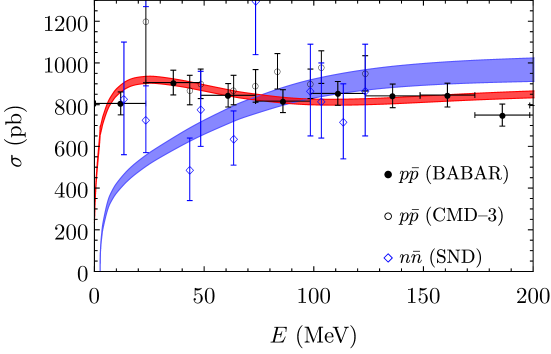
Figure 3: The cross sections of $p\bar{p}$ (thin band) and $n\bar{n}$ (thick band) production as a function of the energy $E$. The experimental data are taken from Refs. (Lees2013, ; Akhmetshin2016, ; Achasov2014, ).

The obtained parameters of the model are shown in Table 1. In Fig. 3 we compare our predictions with the experimental data for the cross sections of $p\bar{p}$ and $n\bar{n}$ pair production in $e^{+}e^{-}$ annihilation in a relatively wide energy region. It is seen that the use of our optical potential results in good agreement with the experimental data.

References

- (1) B. Aubert, et al., Phys. Rev. D 73, 012005 (2006).
- (2) J.P. Lees, et al., Phys. Rev. D 87, 092005 (2013).
- (3) J.P. Lees, et al., Phys. Rev. D 88, 072009 (2013).
- (4) R.R. Akhmetshin, et al., Phys. Lett. B 759, 634 (2016).
- (5) M.N. Achasov, et al., Phys. Rev. D 90, 112007 (2014).
- (6) B. Aubert, et al., Phys. Rev. D 73, 052003 (2006).
- (7) B. Aubert, et al., Phys. Rev. D 76, 092005 (2007).
- (8) R.R. Akhmetshin, et al., Phys. Lett. B 723, 82 (2013).
- (9) P.A. Lukin, et al., Phys. At. Nucl. 78, 353 (2015).
- (10) J.Z. Bai, et al., Phys. Lett. B 510, 75 (2001).
- (11) J. Bai, et al., Phys. Rev. Lett. 91, 022001 (2003).
- (12) M. Ablikim, et al., Phys. Rev. D 80, 052004 (2009).
- (13) M. Ablikim, et al., Eur. Phys. J. C 53, 15 (2008).
- (14) J. P. Alexander, et al., Phys. Rev. D 82, 092002 (2010).
- (15) M. Ablikim, et al., Phys. Rev. Lett. 108, 112003 (2012).
- (16) M. Ablikim, et al., Phys. Rev. D 87, 112004 (2013).
- (17) V.F. Dmitriev and A.I. Milstein, Phys. Lett. B 658, 13 (2007).
- (18) V.F. Dmitriev, A.I. Milstein, and S.G. Salnikov, Phys. At. Nucl. 77, 1173 (2014).
- (19) J. Haidenbauer, X.-W.-W. Kang, and U.-G.-G. Meißner, Nucl. Phys. A 929, 102 (2014).
- (20) J. Haidenbauer, C. Hanhart, X.-W. Kang, and U-G. Meißner, Phys. Rev. D 92, 054032 (2015).
- (21) X.-W. Kang, J. Haidenbauer, and U-G. Meißner, Phys. Rev. D 91, 074003 (2015).
- (22) V.F. Dmitriev, A.I. Milstein, and S.G. Salnikov, Phys. Rev. D 93, 034033 (2016).
- (23) V.F. Dmitriev, A.I. Milstein, and S.G. Salnikov, Phys. Lett. B 760, 139 (2016).
- (24) A.I. Milstein and S.G. Salnikov, Nucl. Phys. A 966, 54 (2017).
- (25) B. El-Bennich, M. Lacombe, B. Loiseau, and S. Wycech, Phys. Rev. C 79, 054001 (2009).
- (26) D. Zhou and R. Timmermans, Phys. Rev. C 86, 044003 (2012).
- (27) X.-W. Kang, J. Haidenbauer, and U-G. Meißner, J. High Energy Phys. 2014, 113 (2014).
- (28) E.P. Solodov, “Study of the hadrons reactions with CMD-3 detector at VEPP-2000 collider”, PoS(EPS-HEP2017)407, DOI: https://doi.org/10.22323/1.314.0407.
- (29) M. B. Voloshin, arXiv:1803.11135 [hep-ph].
- (30) T. Ericson and W. Weise, Pions and nuclei (Clarendon Press, Oxford, 1988).