Anomalous quantum-critical scaling corrections in two-dimensional antiferromagnets
Abstract
We study the Néel–paramagnetic quantum phase transition in two-dimensional dimerized Heisenberg antiferromagnets using finite-size scaling of quantum Monte Carlo data. We resolve the long standing issue of the role of cubic interactions arising in the bond-operator representation when the dimer pattern lacks a certain symmetry. We find non-monotonic (monotonic) size dependence in the staggered (columnar) dimerized model, where cubic interactions are (are not) present. We conclude that there is a new irrelevant field in the staggered model, but, at variance with previous claims, it is not the leading irrelevant field. The new exponent is and the prefactor of the correction is large and comes with a different sign from that of the conventional correction with . Our study highlights competing scaling corrections at quantum critical points.
One of the best understood quantum phase transitions is that between Néel antiferromagnetic (AFM) and quantum paramagnetic ground states in bipartite two- and three-dimensional (2D and 3D) dimerized Heisenberg models with inter- and intra-dimer couplings and sigma ; 3dmap ; millis ; chubukov94 ; always ; thebook . The ground state hosts AFM order when , and there is a critical point at some model dependent . The 3D version of this transition for spins has an experimental realization in TlCuCl3 under high pressure merchant14 ; qin15 . While no 2D realization exists as of yet (though the magnetic field driven transition has been realized bec ), this case has been very important for developing the framework for 2D quantum phase transitions of the Néel AFM state gc . The field theory of the AFM–paramagnetic transition is now well developed, and efficient quantum Monte Carlo (QMC) methods can be used to study ground states of microscopic models with tens of thousands of spins thebook . Many non-trivial predictions for scaling in temperature, frequency, system size, etc., have been tested sandvik94 ; troyer1996 ; ladder ; bilayer ; sen15 ; lohofer15 .
Despite many successes, there are still questions surrounding the 2D AFM–paramagnetic transition. A long-standing unresolved issue is differences observed in QMC calculations between two classes of dimer patterns different ; jiang09 ; unusual ; cubic ; accurate , exemplified by the often studied columnar dimer model (CDM) and the initially less studied staggered dimer model (SDM), both illustrated in Fig. 1. Indications from finite-size scaling of a universality class different from the expected 3D O(3) class in the SDM different led to several follow-up studies jiang09 ; unusual ; cubic ; accurate . The consensus now is that there is no new universality class, as defined by the standard critical exponents. However, because of the lack of a certain local symmetry, cubic interactions arise in the bond-operator description of the SDM, which in the renormalization group corresponds to an irrelevant field that is present neither in the CDM nor in the classical O(3) model cubic . Thus, the SDM contains an interesting quantum effect worthy of further investigations.
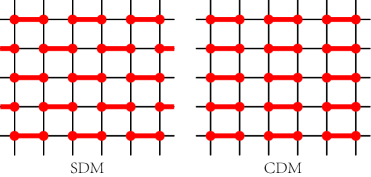
In this Letter we report detailed comparisons of the finite size () scaling corrections of type in the CDM and SDM. While previous works on judiciously chosen observables unusual and lattices with optimized aspect ratios accurate have convincingly demonstrated O(3) universality, the reasons for the unusual scaling behaviors of the SDM have never been adequately explained. In Ref. cubic, , QMC calculations indicated that the exponent of the leading correction is smaller than in the CDM, but the value, in the SDM cubic ; accurate versus the conventional value guida98 ; besteta in the O(3) model and the CDM, is not very different and cannot explain all the observed anomalous finite-size scaling properties of the SDM.
We here study CDM and SDM systems of size up to . Focusing on the scaling corrections, we fix the leading critical exponents at their known O(3) values in our finite-size analysis, which allows us to reliably investigate also subleading corrections. In contrast to the previous studies, we demonstrate that the SDM actually does not have a smaller than the CDM. Instead, the cubic interaction induces the next correction, which has (where the number within parathesis here and henceforth denotes the statistical error in the preceding digit) and a large prefactor of sign different from that of the first correction. This causes non-monotonic finite-size behaviors that were previously either not observed unusual ; cubic or not analyzed properly accurate .
QMC and fitting procedures.—We here use the standard stochastic series expansion QMC method sandvik99 ; thebook for spins and set the inverse temperature at (so that is close to the spinwave velocity accurate ). At a quantum phase transition with dynamic exponent (as is the case here), as long as the temperature does not appear as an independent argument in the scaling function obtained from renormalization group theory. In the case of a dimensionless quantity we have barber ; compost
| (1) |
if is sufficiently close to . Here denotes the irrelevant fields, which we order such that . Useful dimensionless quantities to study in QMC calculations include the Binder ratio , where is the component of the staggered magnetization along the quantization axis, the -normalized spin stiffness constants and (with and referring to the lattice directions), and the uniform susceptibility . We refer to Ref. thebook, for technical details.
To linear order in the first irrelevant field, Eq. (1) can be written as
| (2) |
where and and are scaling functions related to the original . Thus, in the absence of corrections (), a dimensionless quantity is size independent at , and by expanding we see that for different cross each other at . With the scaling correction included, the crossing points only drift toward as , and for two different sizes and one can derive simple expressions for the crossing value and the observable at this point luck ;
| (3a) | |||
| (3b) | |||
where only and depend on . We use as a convenient size ratio allowing for a large number of size pairs , with size series of the form for a range of integers and several choises of . Tests with other reveal no changes in the asymptotics.
We extract the crossings using third-order polynomial fits to ten or more data points in the neighborhood of , with the window reduced as is increased. Such interpolations give reliable crossing points, and statistical errors are computed using bootstrapping. Examples of data with fits are shown in Fig. 2.
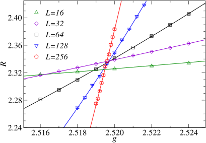
When fitting the crossing points and to their appropriate finite-size scaling forms, the same system size can appear in two pairs, as well as . There are therefore some covariance effects, which we take into account by using the full covariance matrix (computed using bootstrap analysis) in the definition of the goodness of the fit . When jointly fitting to two different quantities, we also account for the associated covariance. For the functional forms, we will go beyond the first-order expansion leading to Eqs. (3), and this will be the key to our findings and conclusions.
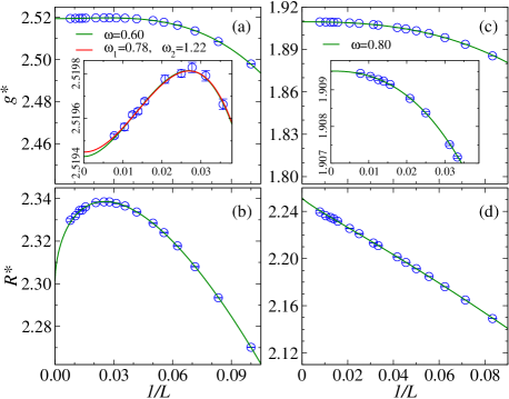
Finite-size scaling.—The size dependence of crossing points is shown in Fig. 3 for both models. A striking feature is the non-monotonic behaviors apparent for the SDM but not present for the CDM. Note here that on the horizontal axis refers to the smaller of the two system sizes used for the crossing points, and the maximums in and are at . In the original discovery of the anomalous behaviors for the SDM different , the systems were smaller and the correct asymptotic behaviors were therefore not reached.
We will first assume that only one irrelevant field is important but treat the corrections beyond the first-order expansion in , Eq. (2). Later we will argue that one has to include also the term in the case of the SDM, while for the CDM is much larger and does not have to be considered. Even with only one irrelevant field, if the associated exponent is small, the higher order terms such as will also be important. As a guide to how far to go, we here compare the previous estimates cubic ; accurate in the SDM with the second correction of the O(3) model, with newman84 , and note that several additional corrections with exponents close to are expected hasen01 . It would then be pointless to go to higher order than in the first irrelevant field, and with we also do not include mixed corrections with and . Thus, for the SDM we use
| (4a) | ||||
| (4b) | ||||
and exclude small systems until good fits are obtained. For the CDM, with , by the above arguments we stop at .
The fitting coefficients and in Eq. (4) are not fully independent of each other but are related because they originate from the same scaling function, Eq. (1). We do not write down the relationships here but fully take them into account in joint fits of the and data. These nonlinear fits are quite demanding and we make use of a slow but reliable stochastic approach optim . The stability of the fits is greatly aided by fixing to its known 3D O(3) value besteta . The resulting curves are shown in Fig. 3. Here, as in all cases below, all data points shown in the figure were included in the fits (with smaller sizes excluded until the fits have acceptable values).
For the CDM, our result for the critical coupling is . The value is consistent with the best previous results, thebook and accurate , but with reduced statistical error. For the correction, we obtain , which agrees with the O(3) value besteta .
For the SDM we obtain . Using rectangular lattices with optimized aspect ratio, a compatible result, , was obtained accurate . For the correction we obtain , which is clearly smaller than the known O(3) value cited above but in good agreement with the values presented in both Refs. cubic and accurate .
| SDM | CDM | |||
|---|---|---|---|---|
Although is universal in the sense that it does not depend on the micro structure of lattice and details of the interactions, it does depend on boundary conditions kamienartz ; selke and aspect ratios accurate . The CDM and SDM have different critical spinwave velocities and, therefore, effectively different time-space aspect ratios even though is the same. This explains the different values in Fig. 3; see also Supplemental Material smcite .
By analyzing also the spin stiffness and the uniform susceptibility in the manner described above, we obtain the results summarized in Tab. 1. The results for the CDM consistently reproduce the known O(3) value of , while in the case of the SDM the different quantities produce a wide range of results. The latter suggests that may not be the true smallest correction exponent in the case of the SDM, but, as also pointed out in Ref. cubic , should be regarded as an “effective exponent” influenced by neglected further corrections. The inability of a single irrelevant field to describe the data is actually not unexpected within the scenario of irrelevant cubic interactions cubic , because the standard leading correction with should still be present and may produce various “effective” scaling behaviors over a limited range of system sizes when combined with the cubic perturbation. Thus, a reliable analysis of the SDM should require at least and .
We can generalize Eqs. (4) to two correction exponents, and , but in that case it is difficult to determine both of them with sufficient precision. However, since the standard leading correction should still be present cubic , we now also fix and only treat as a free parameter. It is then sufficient to go to linear order in the corrections and yet obtain fully acceptable fits. We obtain and for the SDM. The new fitted curve is shown in the inset of Fig. 3(a). The estimate of is a bit higher than the previous value from , but the difference is not statistically significant.
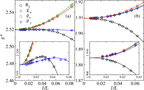
The key result here is clearly that comes out larger than the leading O(3) exponent. It is, however, significantly smaller than the expected second irrelevant exponent with value newman84 ; hasen01 , and it is also less than . The new correction should therefore be due to the cubic interactions cubic in the low-energy theory of the SDM. To test the stability of across different quantities, we also used a slightly different procedure of fitting only to (instead of the joint fit with ) and requiring the same value of for all the quantities considered. We still also fix and but keep free for all individual quantities. The SDM data with fits are displayed in Fig. 4(a), with the resulting and estimates listed in the caption. The fits are statistically good and all four estimates are consistent with the value obtained above. In the case of the CDM, shown Fig. 4(b), we follow the same procedures but replace by and there is no free exponent. This fit is only of marginally acceptable statistical quality even when starting the fits from , indicating some effects still of the higher-order terms that were included in Fig. 3(b). We therefore keep the value from in Tab. 1 as our best estimate for this model.

To further ascertain our conclusions about the SDM, we also consider the squared order parameter itself. Having determined a precise estimate of , we study the scaling of at this point, where we expect
| (5) |
We can then define a size-dependent exponent as
| (6) |
which should scale as
| (7) |
To test this form and extract , we use the known value besteta and fix . As shown in Fig. 5, the form fits the data very well and gives . Here one can again see how access to only system sizes less than could easily lead to the wrong conclusion. A fit with two adjustable exponents gives and , perfectly consistent with the fit with fixed. In the case of the CDM, also shown in Fig. 5, we find that the data are well described with a single correction with the known value of the exponent.
Conclusions.—We have analyzed the SDM under the scenario cubic of an O(3) quantum phase transition with an additional irrelevant perturbation that is absent in the CDM. Our results are consistent with this picture and demand a new scaling correction with exponent that is larger than the also present conventional 3D O(3) exponent but smaller than the next known O(3) exponent. Thus, the cubic interactions in the low-energy theory are formally more irrelevant than previously believed cubic ; accurate , but their effects are important in finite-size scaling of many quantities because of their different signs and larger prefactors of the correction terms (four times larger than the factor of the leading correction in the case of the order parameter), thus giving rise to non-monotonic behaviors.
In addition to resolving the role of the cubic interactions in the class of models represented by the SDM, our study also serves as an example of finite-size behaviors that may at first sight appear puzzling but can be understood once the possibility of competing scaling corrections is recognized. Nonmonotonic scaling has also been observed at the deconfined quantum phase transitions, which has complicated efforts to extract the critical point and exponents shao16 .
Acknowledgements.
Acknowledgments.—We would like to thank Ning Su, Stefan Wessel, and Matthias Vojta for useful discussions. The work of N.M. and D.X.Y. was supported by Grants No. NKRDPC-2017YFA0206203, No. NKRDPC-2018YFA0306001, No. NSFC-11574404, No. NSFC-11275279, No. NSFG-2015A030313176, and the Leading Talent Program of Guangdong Special Projects. H.S. was supported by the China Postdoctoral Science Foundation under Grants No. 2016M600034 and No. 2017T100031. W.G. was supported by NSFC under Grants No. 11775021 and No. 11734002. A.W.S was supported by the NSF under Grant No. DMR-1710170 and by a Simons Investigator Award. Some of the calculations were carried out on Boston University’s Shared Computing Cluster.References
- (1) S. Chakravarty, B. I. Halperin, and D. R. Nelson, Phys. Rev. Lett. 60, 1057 (1988).
- (2) R. R. P. Singh, M. P. Gelfand and D. A. Huse, Phys. Rev. Lett. 61, 2484 (1988).
- (3) A. J. Millis and H. Monien, Phys. Rev. Lett. 70, 2810 (1993).
- (4) A. V. Chubukov, S. Sachdev, and J. Ye, Phys. Rev. B 49, 11919 (1994).
- (5) S. Sachdev, Quantum Phase Transition, 2nd edition (Cambridge University Press, Cambridge, 2011).
- (6) A. W. Sandvik, AIP Conf. Proc. 1297, 135 (2010).
- (7) P. Merchant, B. Normand, K. W. Kramer, M. Boehm, D. F. McMorrow, and C. Rüegg, Nat. Phys. 10, 373 (2014).
- (8) Y. Q. Qin, B. Normand, A. W. Sandvik, and Z. Y. Meng, Phys. Rev. B 92, 214401 (2015).
- (9) T. Giamarchi, C. Rüegg, and O. Tchernyshyov, Nat. Phys. 4, 198 (2008).
- (10) S. Sachdev, Nat. Phys, 4, 173 (2008).
- (11) A. W. Sandvik and D. J. Scalapino, Phys. Rev. Lett. 72, 2777 (1994).
- (12) M. Troyer, H. Kontani, and K. Ueda, Phys. Rev. Lett. 76, 3822 (1996).
- (13) M. Matsumoto, C. Yasuda, S. Todo, and H. Takayama, Phys. Rev. B 65, 014407 (2001).
- (14) L. Wang, K. S. D. Beach, and A. W. Sandvik, Phys. Rev. B 73, 014431 (2006).
- (15) A. Sen, H. Suwa, and A. W. Sandvik, Phys. Rev. B 92, 195145 (2015).
- (16) M. Lohö̈fer, T. Coletta, D. G. Joshi, F. F. Assaad, M.Vojta, S. Wessel, and F. Mila, Phys. Rev. B 92, 245137 (2015).
- (17) S. Wenzel, L. Bogacz and W. Janke, Phys. Rev. Lett. 101,127202 (2008).
- (18) F.-J. Jiang and U. Gerber, J. Stat. Mech. (2009) P09016.
- (19) F.-J. Jiang, Phys. Rev. B 85, 014414 (2012).
- (20) L. Fritz, R. L. Doretto, S. Wessel, S. Wenzel, S. Burdin and M. Vojta, Phy. Rev. B 83,174416 (2011).
- (21) S. Yasuda and S. Todo, Phys. Rev. E 88, 061301(R) (2013).
- (22) R. Guida and J. Zinn-Justin, J. Phys. A: Math. Gen. 31 8103 (1998).
- (23) M. Campostrini, M. Hasenbusch, A. Pelissetto, P. Rossi, and E. Vicari, Phys. Rev. B 65, 144520 (2002).
- (24) A. W. Sandvik, Phys. Rev. B 59, R14157 (1999).
- (25) M. N. Barber, in Phase Transitions and Critical Phenomena, edited by C. Domb and J. L. Lebowitz (Academic Press, New York, 1983), Vol. 8.
- (26) M. Campostrini, A. Pelissetto and E. Vicari, Phys. Rev. B 89, 094516 (2014).
- (27) J. M. Luck, Phys. Rev. B 31, 3069 (1985).
- (28) C. Liu, L. Wang, A. W. Sandvik, Y.-C. Su, and Y.-J. Kao, Phys. Rev. B 82, 060410(R) (2010).
- (29) G. Kamienartz and H. W. J. Blöte, J. Phys. A: Math. Gen. 26, 201 (1993).
- (30) W. Selke, J. Stat. Mech. (2007) P04008.
- (31) See Supplemental Material following the main paper for the dependence of on the space-time aspect ratio.
- (32) K. E. Newman and E. K. Riedel, Phys. Rev. B 30 6615 (1984).
- (33) M. Hasenbusch, J. Phys. A: Math. Gen. 34 8221 (2001).
- (34) H. Shao, W. Guo, and A. W. Sandvik, Science 352, 213 (2016).
I Supplemental Material
Anomalous quantum-critical scaling corrections in two-dimensional antiferromagnets
N. Ma, P. Weinberg, H. Shao, W. Guo, D.-X. Yao, and A. W. Sandvik
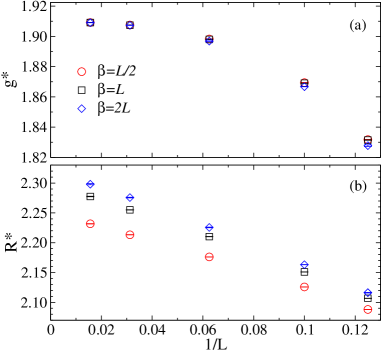
Here we discuss the dependence of the critical Binder ratio on the time-space aspect ratio of the system in the QMC simulations, to explain the fact that the results for the SDM and the CDM in Fig. 3 of the main text do not extrapolate to the same value when . We also comment more broadly on the role of aspect ratios when analyzing quantum phase transitions.
The dependence of the Binder ratio on the spatial aspect ratio in classical systems is well understood kamienartz ; selke , and in quantum systems also acts as an aspect ratio. In addition, the CDM and SDM lack 90∘ lattice rotational invariance and therefore have different velocities of excitations in the two lattice directions. In order to obtain the universal value of , one has to find both the correct spatial aspect ratio , corresponding to the ratio of the two velocities, and the temporal ratio . This was done in Ref. accurate , and the crossing values of the CDM and SDM were shown to indeed be universal, agreeing with the value obtained for the 3D classical Heisenberg model at its critical temperature.
Here we just illustrate the dependence on the temporal ratio in the case of the CDM, keeping the spatial geometry. The results shown in Figure S1 demonstrate that the critical point consistently flows to the same value, while the asymptotic crossing value depends on . We do not extrapolate these results to infinite size, as the purpose is just to illustrate the very clear flows toward incompatible infinite-size values for different ratios. Although the CDM and SDM have the same ratio in the QMC simulations leading to the results in Fig. 3, the effective aspect ratio is still different because of the different spinwave velocities. The two models also have effectively different spatial aspect ratios.
While we agree with Ref. accurate on the point of the common universality of the CDM, SDM, and O(3) models, and the importance of tuning aspect ratios if one desires to observe the universal Binder cumulant, we are not convinced of the practical utility of finding the special aspect ratios and make the system effectively perfectly space-time isotropic. Optimizing the aspect ratios is an additional complication in the simulations, though potentially the symmetry between the directions also could have advantageous effects on the scaling, thoough this is not clear from the results presented so far. In Ref. accurate some non-monotonic behaviors were also seen, i.e., the corrections arising from the cubic interactions do not vanish at the special aspect ratios, which one should also not expect. As we have shown in the main text, one can reach the correct conclusions on the universality class also with lattices and with any fixed reasonable ratio (where one should also keep in mind that the QMC simulation time scales linearly with and with ). The key to understand fully the role of the cubic interactions in the SDM is to realize the importance of two irrelevant fields in the finite-size analysis.