Lensless Wiener-Khinchin telescope based on high-order spatial autocorrelation of thermal light

Abstract

The resolution of a conventional imaging system based on first-order field correlation can be directly obtained from the optical transfer function. However, it is challenging to determine the resolution of an imaging system through random media, including imaging through scattering media and imaging through randomly inhomogeneous media, since the point-to-point correspondence between the object and the image plane in these systems cannot be established by the first-order field correlation anymore. In this paper, from the perspective of ghost imaging, we demonstrate for the first time to our knowledge that the point-to-point correspondence in these imaging systems can be quantitatively recovered from the high-order correlation of light fields, and the imaging capability, such as resolution, of such imaging schemes can thus be derived by analyzing high-order correlation of the optical transfer function. Based on this theoretical analysis, we propose a lensless Wiener-Khinchin telescope based on high-order spatial autocorrelation of thermal light, which can acquire the image of an object by a snapshot via using a spatial random phase modulator. As an incoherent imaging approach illuminated by thermal light, lensless Wiener-Khinchin telescope can be applied in many fields such as X-ray astronomical observations.

Imaging resolution is an important metric of various imaging systems, including microscopy, astronomy, and photography Sheppard (2017); Baker and Kanade (2002); Roggemann et al. (1997); Hao et al. (2013). It is well known that the operating wavelength $\lambda$ and the aperture $D$ of an imaging system are two key parameters for resolution Sheppard (2017); Baker and Kanade (2002). Generally speaking, in conventional imaging systems, where a point-to-point correspondence between the object and the image plane can be established based on first-order field correlation, the resolution can be directly analyzed from a transmission function of the imaging system, and it is proportional to $\lambda/D$. Therefore, a shorter wavelength $\lambda$ and/or a larger aperture $D$ is required for a higher resolution, however, a large aperture leads to demanding requirements on the manufacture of a traditional monolithic optical telescope, which is arduous especially for X-ray imaging.

Recently, emerging systems through random media Choi et al. (2011); Liutkus et al. (2014); Newman and Webb (2014); Yilmaz et al. (2015); Liu et al. (2016); Sahoo et al. (2017); Antipa et al. (2017); Wang and Menon (2015); Bertolotti et al. (2012); Katz et al. (2012, 2014); Yang et al. (2014); Labeyrie (1970); Gezari et al. (1972) have been built, which include imaging through scattering media and imaging through randomly inhomogeneous media. However, it is challenging to determine the resolution of these imaging systems, since the point-to-point correspondence between the object and the image plane in these systems cannot be established by the first-order correlation anymore. In this paper, we show that when the statistical properties of the random media are known as a prior, the resolution of such imaging system can be deduced by analyzing high-order correlation of light fields from the prospective of ghost imaging (GI) Liu et al. (2007); Zhang et al. (2009); Liu et al. (2016). Based on this theoretical analysis, a lensless Wiener-Khinchin telescope is further proposed based on high-order spatial autocorrelation of thermal light, which can acquire the image of the object in a single shot by using a spatial random phase modulator (SRPM). We theoretically and experimentally demonstrate that different from conventional imaging systems, the resolution of lensless Wiener-Khinchin telescope not only depends on the aperture of SRPM, but also on the statistical properties of it. The influence of signal bandwidth is also investigated. Moreover, experimental results for both far away and equivalent infinity far away imaging proves the feasibility of the proposed lensless Wiener-Khinchin telescope in astronomical observations.

The proposed lensless Wiener-Khinchin telescope (Fig. 1) consists of a SRPM and a charge-coupled device (CCD) detector, which detects the intensity distribution of the modulated light field. The object is illuminated by a thermal light source.

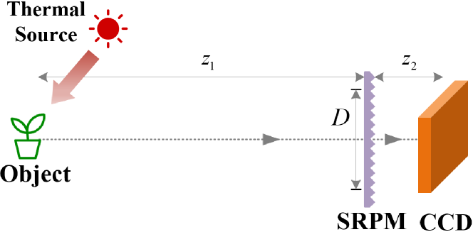
Figure 1: Schematic of a lensless Wiener-Khinchin telescope. $D$ is the diameter of the SRPM. $z_{1}$ and $z_{2}$ are distances from the object and detection planes to the SRPM, respectively.

For incoherent imaging Goodman (2005a), the spatial intensity distribution detected by the CCD detector is

$$I_{t}(r)=\int_{-\infty}^{\infty}{I_{0}(r_{0})h_{I}(r;r_{0})dr_{0}}\quad,$$ (1)

where $I_{0}(r_{0})$ is the intensity distribution in the object plane, $h_{I}(r;r_{0})=h_{E}(r;r_{0})h_{E}^{*}(r;r_{0}^{\prime})$ is the incoherent intensity impulse response function, $h_{E}(r;r_{0})$ is the point-spread function (PSF) of the imaging system.

Considering the spatial random phase modulator for thermal light as an ergodic process, the second-order spatial autocorrelation of the measured light field is Cheng and Han (2004); Shapiro and Boyd (2012)

$$\begin{split}&G_{{I_{t}}}^{(2)}\left({r+\Delta r,r}\right)\\ &=\left\langle{E_{t}^{*}\left({r+\Delta r}\right)E_{t}^{*}\left(r\right){E_{t}}\left(r\right){E_{t}}\left({r+\Delta r}\right)}\right\rangle_{r}\\ &=\overline{\left\{E_{t}^{*}\left({r+\Delta r}\right)E_{t}^{*}\left(r\right){E_{t}}\left(r\right){E_{t}}\left({r+\Delta r}\right)\right\}}_{s}\\ &=\overline{\left\{{I_{t}}\left(r\right){I_{t}}\left({r+\Delta r}\right)\right\}}_{s}\end{split}$$ (2)

where $\left\langle\cdot\right\rangle_{r}$ is the spatial average over the coordinate $r$, and $\overline{\{\cdot\}}_{s}$ is the ensemble average of the SRPM. Plugging Eq. (1) into Eq. (2), we have

$$\begin{split}G_{{I_{t}}}^{(2)}\left({r+\Delta r,r}\right)=\iint_{-\infty}^{\infty}&G_{h}^{(2)}(r+\Delta r,r_{0}+\Delta r_{0};r,r_{0})\\ &I_{0}(r_{0}+\Delta r_{0})I_{0}(r_{0})dr_{0}d\Delta r_{0},\end{split}$$ (3)

where

$$\begin{split}&G_{h}^{(2)}(r+\Delta r,r_{0}+\Delta r_{0};r,r_{0})=\\ &\overline{\left\{h_{E}^{*}(r+\Delta r;r_{0}+\Delta r_{0})h_{E}^{*}(r;r_{0})h_{E}(r;r_{0})h_{E}(r+\Delta r;r_{0}+\Delta r_{0})\right\}}_{s}\\ \end{split}$$ (4)

is the second-order correlation function of PSFs.

According to the Central Limit Theorem Goodman (2007), the light field $h_{E}(r;r_{0})$ through the spatial random phase modulator obeys the complex circular Gaussian distribution in spatial domain Goodman (2007), and $G_{h}^{(2)}(r+\Delta r,r_{0}+\Delta r_{0};r,r_{0})$ can be written as Goodman (2015)

$$\begin{split}&G_{h}^{(2)}(r+\Delta r,r_{0}+\Delta r_{0};r,r_{0})\\ &=B\left[1+g_{h}^{(2)}(r+\Delta r,r_{0}+\Delta r_{0};r,r_{0})\right]\end{split}$$ (5)

with $B=\overline{\left\{h(r;r_{0})\right\}}_{s}\overline{\left\{h(r+\Delta r;r_{0}+\Delta r_{0})\right\}}_{s}$, and

$$\begin{split}&g_{h}^{(2)}(r+\Delta r,r_{0}+\Delta r_{0};r,r_{0})\\ &=\dfrac{\left|\overline{\left\{h_{E}^{*}(r+\Delta r;r_{0}+\Delta r_{0})h_{E}(r;r_{0})\right\}}_{s}\right|^{2}}{B}\\ \end{split}$$ (6)

is the normalized second-order correlation of PSFs.

For Fresnel diffraction, the PSF of a lensless Wiener-Khinchin telescope is

$$\begin{split}&h_{E}(r;r_{0})=\dfrac{\exp\{{j2\pi(z_{1}+z_{2})/\lambda}\}}{-\lambda^{2}z_{1}z_{2}}\exp\left\{{\dfrac{j\pi(r-r_{0})^{2}}{\lambda(z_{1}+z_{2})}}\right\}\\ &\int_{-\infty}^{\infty}P(r_{m})t(r_{m})\exp\left\{\frac{j\pi(z_{1}+z_{2})}{\lambda z_{1}z_{2}}\left[r_{m}-\frac{z_{1}r+z_{2}r_{0}}{z_{1}+z_{2}}\right]^{2}\right\}dr_{m},\end{split}$$ (7)

where $P(r_{m})$ and $t(r_{m})=\exp{\left[j2\pi(n-1){\eta(r_{m})}/{\lambda}\right]}$ are the pupil function and the transmission function of SRPM, respectively, while $\eta(r_{m})$ and $n$ are its height and refractive index, respectively. The space translation invariance of system in space (also known as memory effect Feng et al. (1988); Osnabrugge et al. (2017)) is required for the Fresnel approximation Goodman (2005b). Since the target of a telescope is very small compared with the imaging distance, the memory effect is satisfied in lensless Wiener-Khinchin telescope.

In general, the height ensemble average ${R_{\eta}}\left({{r_{m}},{r_{n}}}\right)$ of SRPM obeys the following mathematical form Sinha et al. (1988)

$$\begin{split}&{R_{\eta}}\left({{r_{m}},{r_{n}}}\right)=\overline{\left\{\eta\left({{r_{m}}}\right)\eta\left({{r_{n}}}\right)\right\}}_{s}\\ &={\omega^{\rm{2}}}\exp\left\{{-{{\left({\frac{{{r_{m}}-{r_{n}}}}{\zeta}}\right)}^{2}}}\right\}={R_{\eta}}\left({\Delta{r_{m}}}\right),\quad\Delta{r_{m}}{\rm{=}}{r_{m}}-{r_{n}},\end{split}$$ (8)

where $\omega$ and $\zeta$ are the height standard deviation and the transverse correlation length of SRPM, respectively. Substituting Eq. (7) and Eq. (8) into Eq. (6) yields (see Supplement 1 for details)

$$\begin{split}&g_{h}^{(2)}(r+\Delta r,r_{0}+\Delta r_{0};r,r_{0})\\ &\approx\left|\left\{{\exp\left\{-2\left[\dfrac{2\pi(n-1)}{\lambda}\right]^{2}\left[\omega^{2}-R_{\eta}\left(\dfrac{2\lambda z_{1}z_{2}}{z_{1}+z_{2}}\nu\right)\right]\right\}}\right.\right.\\ &\left.\left.\otimes\mathcal{F}\left\{{\left|P\left(\mu+\mu_{0}\right)\right|^{2}}\right\}_{\mu\to\nu}\right\}_{\dfrac{z_{1}\Delta r+z_{2}\Delta r_{0}}{2\lambda z_{1}z_{2}}}\right|^{2}\\ &=g_{h}^{(2)}\left(\dfrac{z_{1}\Delta r+z_{2}\Delta r_{0}}{2\lambda z_{1}z_{2}}\right),\end{split}$$ (9)

where $\mathcal{F}\{\cdots\}_{\mu\to\nu}$ represents the Fourier transform of the function with the variable $\mu$ and the transformed function variable is $\nu$, and

$$\mu_{0}=\dfrac{z_{1}(2r+\Delta r)+z_{2}\left(2r_{0}+\Delta r_{0}\right)}{2\left(z_{1}+z_{2}\right)}.$$ (10)

Taking Eqs. (5) and (9) into Eq. (3), we have

$$\begin{split}G_{{I_{t}}}^{(2)}\left({r+\Delta r,r}\right)\approx B\left\{\left[1+g_{h}^{(2)}\left(\dfrac{\Delta r_{0}}{2\lambda z_{1}}\right)\right]\otimes{G_{{I_{0}}}^{(2)}\left({r_{0}+\Delta r_{0},r_{0}}\right)}\right\}_{-\dfrac{z_{1}}{z_{2}}\Delta r},\end{split}$$ (11)

where

$$\begin{split}G_{{I_{0}}}^{(2)}\left({r_{0}+\Delta r_{0},r_{0}}\right)=\int_{-\infty}^{\infty}{I_{0}(r_{0})I_{0}\left(r_{0}+\Delta r_{0}\right)dr_{0}},\end{split}$$ (12)

and

$$\begin{split}&g_{h}^{(2)}\left(\dfrac{\Delta r_{0}}{2\lambda z_{1}}\right)\\ &=\left|\left\{{\exp\left\{-2\left[\dfrac{2\pi(n-1)}{\lambda}\right]^{2}\left[\omega^{2}-R_{\eta}\left(\dfrac{2\lambda z_{1}z_{2}}{z_{1}+z_{2}}\nu\right)\right]\right\}}\right.\right.\\ &\left.\left.\otimes\mathcal{F}\left\{{\left|P\left(\mu+\mu_{0}\right)\right|^{2}}\right\}_{\mu\to\nu}\right\}_{\dfrac{\Delta r_{0}}{2\lambda z_{1}}}\right|^{2}.\end{split}$$ (13)

According to the Wiener-Khinchin theorem for deterministic signals Cohen (1998)(also known as autocorrelation theorem Goodman (2005c)), we have

$$\begin{split}&G_{{I_{0}}}^{(2)}\left({r_{0}+\Delta r_{0},r_{0}}\right)=\mathcal{F}^{-1}\left\{{\left|{\mathcal{F}\left\{{I_{0}(r_{0})}\right\}_{r_{0}\to f_{0}}}\right|^{2}}\right\}_{f_{0}\to\Delta r_{0}}.\end{split}$$ (14)

Substituting Eq. (14) into Eq. (11), we obtain

$$\begin{split}G_{{I_{t}}}^{(2)}&\left({r+\Delta r,r}\right)\propto\left\{\left[1+g_{h}^{(2)}\left(\dfrac{\Delta r_{0}}{2\lambda z_{1}}\right)\right]\right.\\ &\left.\otimes{\mathcal{F}^{-1}\left\{{\left|{\mathcal{F}\left\{{I_{0}(r_{0})}\right\}_{r_{0}\to f_{0}}}\right|^{2}}\right\}_{f_{0}\to\Delta r_{0}}}\right\}_{-\dfrac{z_{1}}{z_{2}}\Delta r}.\end{split}$$ (15)

Eq. (15) indicates that the energy spectral density ${\left|{\mathcal{F}\left\{{I_{0}(r_{0})}\right\}_{r_{0}\to f_{0}}}\right|^{2}}$ of the intensity distribution $I_{0}(r_{0})$ on the object plane can be separated from $G_{{I_{t}}}^{(2)}\left({r+\Delta r,r}\right)$, and the resolution is determined by $g_{h}^{(2)}\left(\dfrac{\Delta r_{0}}{2\lambda z_{1}}\right)$. The image of ${I_{0}}(r_{0})$ can be reconstructed by utilizing phase retrieval algorithms Fienup (1978, 1982); Liu et al. (2015); Shechtman et al. (2015). Here, only amplitude information of the target is interested, which can be used as a constraint to significantly improve the speed and quality of reconstruction Ying et al. (2008).

To quantify the imaging system, the relationship between the field of view (FOV), the resolution and the spatial random phase modulator is analyzed.

The FOV of lensless Wiener-Khinchin telescope is limited by the memory effect range of the imaging system. Considering the height standard deviation $\omega$ of the SRPM, the normalized second-order correlation function of light fields between different incident angles without transverse translation is (see Supplement 1 for details)

$$\begin{split}g_{\theta}^{(2)}\left({\Delta\theta}\right)\approx\exp\left\{{-{{\left({\dfrac{{\pi n\omega}}{\lambda}\sin^{2}\left(\Delta\theta\right)}\right)}^{2}}}\right\},\end{split}$$ (16)

where $\Delta\theta$ is the variation of the incident angle. According to Eq. (16), the FOV is proportional to $\dfrac{\lambda}{\omega}$.

In addition, Eq. (15) leads to a limitation of the FOV,

$$FOV<\dfrac{L}{z_{2}}$$ (17)

with $L$ denoting the CCD detector size. This equation indicates that FOV is also limited by the CCD detector size. In order to obtain a large FOV, the CCD detector size of lensless Wiener-Khinchin telescope is required to be much larger than $\dfrac{\lambda z_{2}}{\omega}$ in Eq. (16).

Eq. (13) indicates that the resolution not only depends on the aperture of the SRPM, but also the statistical properties of it. According to the convolution operation in $g_{h}^{(2)}\left(\dfrac{\Delta r_{0}}{2\lambda z_{1}}\right)$, we discuss two simple cases below, where the resolution is mainly limited by the aperture and the statistical properties of the SRPM, respectively.

Case 1: resolution is mainly limited by the aperture.

When the full width at half maximum (FWHM) of $\small\exp\left\{-2\left[\dfrac{2\pi(n-1)}{\lambda}\right]^{2}\left[\omega^{2}-R_{\eta}\left(\dfrac{2\lambda z_{1}z_{2}}{z_{1}+z_{2}}\nu\right)\right]\right\}$ is much smaller than the FWHM of $\mathcal{F}\left\{{\left|P\left(\mu+\mu_{0}\right)\right|^{2}}\right\}_{\mu\to\nu}$, we have

$$\begin{split}g_{h}^{(2)}\left(\dfrac{\Delta r_{0}}{2\lambda z_{1}}\right)\approx\left|\mathcal{F}\left\{{\left|P\left(\mu\right)\right|^{2}}\right\}_{\mu\to-\dfrac{\Delta r_{0}}{2\lambda z_{1}}}\right|^{2}.\end{split}$$ (18)

For a circle aperture of the SRPM, $P(\mu)=\mathrm{circ}\left(\dfrac{\mu}{D}\right)$, and this leads to

$$\begin{split}g_{h}^{(2)}\left(\dfrac{\Delta r_{0}}{2\lambda z_{1}}\right)\propto\left[{\dfrac{J_{1}(\dfrac{2\pi D\Delta r_{0}}{z_{1}\lambda})}{\dfrac{2\pi D\Delta r_{0}}{z_{1}\lambda}}}\right]^{2}.\end{split}$$ (19)

In this case, the resolution of the lensless Wiener-Khinchin telescope is proportional to $\lambda z_{1}/D$.

Case 2: resolution is mainly limited by the statistical properties.

When the FWHM of $\exp\left\{-2\left[\dfrac{2\pi(n-1)}{\lambda}\right]^{2}\left[\omega^{2}-R_{\eta}\left(\dfrac{2\lambda z_{1}z_{2}}{z_{1}+z_{2}}\nu\right)\right]\right\}$ is much larger than the FWHM of $\mathcal{F}\left\{{\left|P\left(\mu+\mu_{0}\right)\right|^{2}}\right\}_{\mu\to\nu}\quad$,

$$\begin{split}&g_{h}^{(2)}\left(\dfrac{\Delta r_{0}}{2\lambda z_{1}}\right)\approx\exp\left\{-4\left[\dfrac{2\pi(n-1)\omega z_{2}\Delta r_{0}}{\lambda\left(z_{1}+z_{2}\right)\zeta}\right]^{2}\right\}\quad,\end{split}$$ (20)

with the first-order approximation. In this case, the resolution is proportional to $\left(1+\dfrac{z_{1}}{z_{2}}\right)\dfrac{\lambda\zeta}{(n-1)\omega}$.

For digital images, the reconstruction is also affected by the pixel size of the CCD detector. Due to Eq. (14), the pixel size $P_{CCD}$ of the CCD detector is required by

$$P_{CCD}<\dfrac{z_{2}}{Mz_{1}}g_{h}^{(2)}\left(\dfrac{\Delta r_{0}}{2\lambda z_{1}}\right),$$ (21)

where $M$ denotes a split number for discrimination of resolution.

The experimental setup is shown in Fig. 2. An object is illuminated by a xenon lamp. The reflected light is filtered by a narrow-band filter, and modulated by a SRPM with a height standard deviation $\omega=1$ $\mu$m, a transverse correlation length $\zeta=44$ $\mu$m and the refractive index $n=1.46$, and then relayed by a lens with a magnification factor $\beta=10$ and a numerical aperture $N.A.=0.25$ onto a CCD detector (APGCCD) with a pixel size 13 $\mu$m $\times$ 13 $\mu$m, which records the magnified intensity distribution. The lens is only used to amplify the intensity distribution to match the pixel size of the CCD detector, and is not necessary in some conditions.

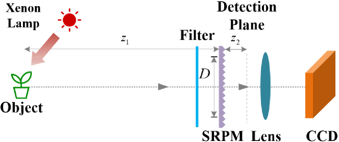
Figure 2: Experimental setup of lensless Wiener-Khinchin telescope.

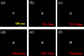
Figure 3: Experimental results with different narrow-band filters. (a) A photograph of the double slit, where a yellow scale bar is inserted in the low right corner. Reconstructed images with different narrow-band filters: (b) $\lambda=532$ nm, $w=$ 3 nm, (c) $\lambda=532$ nm, $w=$ 10 nm, (d) $\lambda=550$ nm, $w=$ 10 nm, (e)$\lambda=550$ nm, $w=$ 25 nm, (f) $\lambda=550$ nm, $w=$ 50 nm.

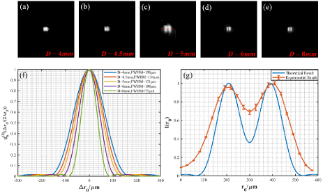
Figure 4: Resolution at different apertures of the spatial random phase modulator. Reconstructed images with different apertures: (a) D= 4 mm, (b) D= 4.5 mm, (c) D= 5 mm, (d) D= 6 mm, (e) D= 8 mm. (f) The theoretical resolutions. (g) A comparison between theoretical and experimental resolutions at $D$= 5 mm, and the red line is a cross-section denoted by the dash line in Fig. 4(c).

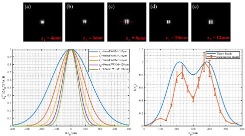
Figure 5: Resolution at different $z_{2}$. Reconstructed images with different $z_{2}$: (a) $z_{2}=$ 4 mm, (b) $z_{2}=$ 6 mm, (c) $z_{2}=$ 8 mm, (d) $z_{2}=$ 10 mm, (e) $z_{2}=$ 12 mm. (f) The theoretical resolutions. (g) A comparison between theoretical and experimental resolutions at $z_{2}$= 8 mm, and the red line is a cross-section denoted by the dash line in Fig. 5(c).

In order to analyze the resolution of the system, a double slit (shown in Fig. 3(a)) is selected. Since the image is obtained from the second-order spatial autocorrelation of thermal light, the temporal coherence is not strictly required. But the temporal coherence of the light field still affects the contrast of the spatial fluctuating pseudo-thermal light due to the dispersion of the spatial random phase modulator. The reflected light from the object is filtered by a narrow-band filter, whose central wavelength $\lambda$ is either 532 nm or 550 nm, and its bandwidth $w$ varies among 3 nm, 10 nm, 25 nm and 50 nm, when $z_{1}=$ 0.15 m, $z_{2}=$ 12 mm, and $D=$ 8mm. The results with the same phase retrieval algorithm Liu et al. (2015) are shown in Fig. 3. The experimental results show that the situation is better for narrow band light. In subsequent experiments, a narrow-band filter with a center wavelength $\lambda=$ 532 nm and a bandwidth $w=$ 10 nm is selected.

To verify Eq. (19) in experiment, the aperture size is changed. Images with five different apertures $D=$ 4 mm, 4.5 mm, 5 mm, 6 mm, 8 mm are obtained, respectively, while $z_{1}=1.1$ m and $z_{2}=60$ mm are selected in accordance with Case 1 (see Fig. 4(a)-(e)). According to Eq. (18), the theoretical resolutions with different apertures are shown in Fig. 4(f), where FWHMs for $D=$ 4 mm, 4.5 mm, 5 mm, 6 mm and 8 mm are 150 $\mu$m, 134 $\mu$m, 121 $\mu$m, 100 $\mu$m and 75 $\mu$m, respectively. Fig. 4(g) shows a comparison of theoretical and experimental resolutions at $D=$ 5 mm, where the red line is a cross-section denoted by the dash line in Fig. 4(c). The experimental results show that the double slit can be distinguished at $D=5$ mm, which agrees well with theoretical results.

In Case 2, the resolution is mainly affected by the statistical properties of SRPM, which leads to a limitation of $z_{2}$ based on Eq. (20). Five different $z_{2}$ (4 mm, 6 mm, 8 mm, 10 mm, 12 mm) are selected, and the reconstructed images are shown in Fig. 5(a)-(e), while $z_{1}=0.3$ m and $D=8$ mm. The corresponding theoretical resolutions are shown in Fig. 5(f), where FWHMs for $z_{2}=$ 4 mm, 6 mm, 8 mm, 10 mm and 12 mm are 313 $\mu$m, 211 $\mu$m, 160 $\mu$m, 129 $\mu$m and 108 $\mu$m, respectively. Fig. 5(g) shows a comparison of theoretical and experimental resolutions at $z_{2}=$ 8 mm, where the red line is the cross-section denoted by the dash line in Fig. 5(c). The results show that the double slit can be distinguished at $z_{2}=$ 8 mm.

To further verify the imaging capability of lensless Wiener-Khinchin telescope, two targets, a letter $\pi$ and a panda toy, are imaged, respectively. Different system parameters are selected at $D=$ 8 mm. For the ‘$\pi$’, $z_{1}=$ 0.5 m, $z_{2}=$ 2 mm, and for the ‘panda’, $z_{1}=$ 1.5 m, $z_{2}=$ 3 mm. Both reconstructed images are shown in Fig. 6.

For astronomical observations, the distance $z_{1}$ is nearly infinitely far away, which means $z_{1}\gg z_{2}$, so the resolution $g_{h}^{(2)}\left(\dfrac{\Delta r_{0}}{2\lambda z_{1}}\right)$ in Eq. (13) is approximated to

$$\begin{split}&g_{h}^{(2)}\left(\dfrac{\Delta r_{0}}{2\lambda z_{1}}\right)\propto\left|\left\{{\exp\left\{-2\left[\dfrac{2\pi(n-1)}{\lambda}\right]^{2}\left[\omega^{2}-R_{\eta}\left(2\lambda z_{2}\nu\right)\right]\right\}}\right.\right.\\ &\qquad\qquad\qquad\left.\left.\otimes\mathcal{F}\left\{{\left|P\left(\mu\right)\right|^{2}}\right\}_{\mu\to\nu}\right\}_{\dfrac{\Delta r_{0}}{2\lambda z_{1}}}\right|^{2}.\end{split}$$ (22)

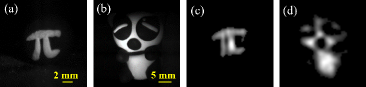
Figure 6: Imaging a letter $\pi$ and a panda toy. (a) and (b) are photographs, where a yellow scale bar is inserted in the low right corner, respectively. (c) and (d) are reconstructed images, respectively.

A capital ‘GI’ is placed on the focal plane of an optical lens before the SRPM to experimentally simulate the target placed infinite far away. The reconstructed image is shown in Fig. 7. Experimental results of Figs. 6 and 7 prove the feasibility of lensless Wiener-Khinchin telescope in astronomical observations.

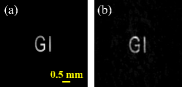
Figure 7: Imaging an object placed equivalent infinite far away. (a) A photograph of the target, where a yellow scale bar is inserted in the low right corner, (b) reconstructed image.

In conclusion, we present a theoretical framework for imaging schemes through random media, and propose lensless Wiener-Khinchin telescope based on high-order correlation of thermal light. The attempt to extract spatial information of an object from high-order correlation of light fields can be traced back to the famous HBT experiment in 1956 Brown and Twiss (1956); Smith and Shih (2018), which is based on the second-order autocorrelation of light fields, and GI proposed in 1995, which is based on second-order mutual-correlation of light fields between the reference and test arms Strekalov et al. (1995). HBT experiment and many of the early works of GI Valencia et al. (2005); Zhang et al. (2005) perform ensemble statistics of the temporal fluctuating light field in time domain, which requires that the temporal resolution of the detector is close to or less than the coherence time of the light field Liu et al. (2014). In contrast, by modulating true thermal light such as sunlight into a spatially fluctuating pseudo-thermal light field through a spatial random phase modulator Liu et al. (2016), lensless Wiener-Khinchin telescope calculates the ensemble statistics of the spatially fluctuating pseudo-thermal light field in spatial domain, therefore, the detection of the temporal intensity fluctuation is not required.

On the other hand, from the viewpoint of the intensity autocorrelation, single-shot imaging through scattering layers and around corners via speckle correlations presented by Katz et al. Katz et al. (2014) didn’t consider the effects of diffraction through the random phase modulation, and then the resolution of the imaging system can not be quantitatively calculated. By analyzing the spatial high-order correlation of light fields, the resolution is derived and experimentally verified in lensless Wiener-Khinchin telescope. The quantitative description of the imaging quality makes such imaging systems not only be demonstrated, but also be designed in practical applications.

Compared with lensless compressive sensing imaging Huang et al. (2013); Antipa et al. (2017); Asif et al. (2017) and lensless GI Chen et al. (2009); Liu et al. (2014); Yu et al. (2016), neither a measurement matrix nor a calibration process is required. Thus lensless Wiener-Khinchin telescope has conspicuous advantages in applications such as X-ray astronomical observations, where the measurement matrix or the calibration for an unknown imaging distance is difficult and inaccurate. The cancellation of calibration also results in lower requirements in system stability. Moreover, considering the scattering media or the randomly inhomogeneous media as a spatial random phase modulator, lensless Wiener-Khinchin telescope may also open a door to quantitatively describe imaging through scattering media or randomly inhomogeneous media Choi et al. (2011); Liutkus et al. (2014); Newman and Webb (2014); Yilmaz et al. (2015); Liu et al. (2016); Sahoo et al. (2017); Antipa et al. (2017); Wang and Menon (2015); Bertolotti et al. (2012); Katz et al. (2012, 2014); Yang et al. (2014); Labeyrie (1970); Gezari et al. (1972).

Funding

National Key Research and Development Program of China (2017YFB0503303). Hi-Tech Research and Development Program of China (2013AA122902 and 2013AA122901).

References

References

- Sheppard (2017) C. J. R. Sheppard, Microscopy Research and Technique 80, 590 (2017).
- Baker and Kanade (2002) S. Baker and T. Kanade, IEEE Transactions on Pattern Analysis and Machine Intelligence 24, 1167 (2002).
- Roggemann et al. (1997) M. C. Roggemann, B. M. Welsh, and R. Q. Fugate, Reviews of Modern Physics 69, 437 (1997).
- Hao et al. (2013) X. Hao, C. Kuang, Z. Gu, Y. Wang, S. Li, Y. Ku, Y. Li, J. Ge, and X. Liu, Light: Science & Applications 2, e108 (2013).
- Choi et al. (2011) Y. Choi, T. D. Yang, C. Fang-Yen, P. Kang, K. J. Lee, R. R. Dasari, M. S. Feld, and W. Choi, Physical Review Letters 107 (2011), 10.1103/physrevlett.107.023902.
- Liutkus et al. (2014) A. Liutkus, D. Martina, S. Popoff, G. Chardon, O. Katz, G. Lerosey, S. Gigan, L. Daudet, and I. Carron, Scientific Reports 4 (2014), 10.1038/srep05552.
- Newman and Webb (2014) J. A. Newman and K. J. Webb, Physical Review Letters 113 (2014), 10.1103/physrevlett.113.263903.
- Yilmaz et al. (2015) H. Yilmaz, E. G. van Putten, J. Bertolotti, A. Lagendijk, W. L. Vos, and A. P. Mosk, Optica 2, 424 (2015).
- Liu et al. (2016) Z. Liu, S. Tan, J. Wu, E. Li, X. Shen, and S. Han, Scientific Reports 6 (2016), 10.1038/srep25718.
- Sahoo et al. (2017) S. K. Sahoo, D. Tang, and C. Dang, Optica 4, 1209 (2017).
- Antipa et al. (2017) N. Antipa, G. Kuo, R. Heckel, B. Mildenhall, E. Bostan, R. Ng, and L. Waller, Optica 5, 1 (2017).
- Wang and Menon (2015) P. Wang and R. Menon, Optica 2, 933 (2015).
- Bertolotti et al. (2012) J. Bertolotti, E. G. van Putten, C. Blum, A. Lagendijk, W. L. Vos, and A. P. Mosk, Nature 491, 232 (2012).
- Katz et al. (2012) O. Katz, E. Small, and Y. Silberberg, Nature Photonics 6, 549 (2012).
- Katz et al. (2014) O. Katz, P. Heidmann, M. Fink, and S. Gigan, Nature Photonics 8, 784 (2014).
- Yang et al. (2014) X. Yang, Y. Pu, and D. Psaltis, Optics Express 22, 3405 (2014).
- Labeyrie (1970) A. Labeyrie, Astron. Astrophys. 6, 85 (1970).
- Gezari et al. (1972) D. Y. Gezari, A. Labeyrie, and R. V. Stachnik, The Astrophysical Journal 173, L1 (1972).
- Liu et al. (2007) H. Liu, J. Cheng, and S. Han, Journal of Applied Physics 102, 103102 (2007).
- Zhang et al. (2009) P. Zhang, W. Gong, X. Shen, D. Huang, and S. Han, Optics Letters 34, 1222 (2009).
- Goodman (2005a) J. W. Goodman, Introduction to Fourier optics, 132-134 (Roberts and Company Publishers, 2005).
- Cheng and Han (2004) J. Cheng and S. Han, Physical Review Letters 92 (2004), 10.1103/physrevlett.92.093903.
- Shapiro and Boyd (2012) J. H. Shapiro and R. W. Boyd, Quantum Information Processing 11, 949 (2012).
- Goodman (2007) J. W. Goodman, Speckle phenomena in optics: theory and applications, 9-12 (Roberts and Company Publishers, 2007).
- Goodman (2015) J. W. Goodman, Statistical optics, 44 (John Wiley & Sons, New York, 2015).
- Feng et al. (1988) S. Feng, C. Kane, P. A. Lee, and A. D. Stone, Physical Review Letters 61, 834 (1988).
- Osnabrugge et al. (2017) G. Osnabrugge, R. Horstmeyer, I. N. Papadopoulos, B. Judkewitz, and I. M. Vellekoop, Optica 4, 886 (2017).
- Goodman (2005b) J. W. Goodman, Introduction to Fourier optics, 66-67 (Roberts and Company Publishers, 2005).
- Sinha et al. (1988) S. K. Sinha, E. B. Sirota, S. Garoff, and H. B. Stanley, Physical Review B 38, 2297 (1988).
- Cohen (1998) L. Cohen, in Proceedings of the 1998 IEEE International Conference on Acoustics, Speech and Signal Processing, ICASSP 98 (Cat. No.98CH36181) (IEEE, 1998).
- Goodman (2005c) J. W. Goodman, Introduction to Fourier optics, 8-9 (Roberts and Company Publishers, 2005).
- Fienup (1978) J. R. Fienup, Optics Letters 3, 27 (1978).
- Fienup (1982) J. R. Fienup, Applied Optics 21, 2758 (1982).
- Liu et al. (2015) X. Liu, J. Wu, W. He, M. Liao, C. Zhang, and X. Peng, Optics Express 23, 18955 (2015).
- Shechtman et al. (2015) Y. Shechtman, Y. C. Eldar, O. Cohen, H. N. Chapman, J. Miao, and M. Segev, IEEE Signal Processing Magazine 32, 87 (2015).
- Ying et al. (2008) G. Ying, Q. Wei, X. Shen, and S. Han, Optics Communications 281, 5130 (2008).
- Brown and Twiss (1956) R. H. Brown and R. Q. Twiss, Nature 177, 27 (1956).
- Smith and Shih (2018) T. A. Smith and Y. Shih, Physical Review Letters 120 (2018), 10.1103/physrevlett.120.063606.
- Strekalov et al. (1995) D. V. Strekalov, A. V. Sergienko, D. N. Klyshko, and Y. H. Shih, Physical Review Letters 74, 3600 (1995).
- Valencia et al. (2005) A. Valencia, G. Scarcelli, M. D’Angelo, and Y. Shih, Physical Review Letters 94 (2005), 10.1103/physrevlett.94.063601.
- Zhang et al. (2005) D. Zhang, Y. H. Zhai, L. A. Wu, and X. H. Chen, Optics Letters 30, 2354 (2005).
- Liu et al. (2014) X. F. Liu, X. H. Chen, X. R. Yao, W. K. Yu, G. J. Zhai, and L. A. Wu, Optics Letters 39, 2314 (2014).
- Huang et al. (2013) G. Huang, H. Jiang, K. Matthews, and P. Wilford, in 2013 IEEE International Conference on Image Processing (IEEE, 2013).
- Asif et al. (2017) M. S. Asif, A. Ayremlou, A. Sankaranarayanan, A. Veeraraghavan, and R. G. Baraniuk, IEEE Transactions on Computational Imaging 3, 384 (2017).
- Chen et al. (2009) X. H. Chen, Q. Liu, K. H. Luo, and L. A. Wu, Optics Letters 34, 695 (2009).
- Yu et al. (2016) H. Yu, R. Lu, S. Han, H. Xie, G. Du, T. Xiao, and D. Zhu, Physical Review Letters 117 (2016), 10.1103/physrevlett.117.113901.