Information Propagation Analysis of Social Network Using the Universality of Random Matrix

Abstract

Spectral graph theory gives an algebraical approach to analyze the dynamics of a network by using the matrix that represents the network structure. However, it is not easy for social networks to apply the spectral graph theory because the matrix elements cannot be given exactly to represent the structure of a social network. The matrix element should be set on the basis of the relationship between persons, but the relationship cannot be quantified accurately from obtainable data (e.g., call history and chat history). To get around this problem, we utilize the universality of random matrix with the feature of social networks. As such random matrix, we use normalized Laplacian matrix for a network where link weights are randomly given. In this paper, we first clarify that the universality (i.e., the Wigner semicircle law) of the normalized Laplacian matrix appears in the eigenvalue frequency distribution regardless of the link weight distribution. Then, we analyze the information propagation speed by using the spectral graph theory and the universality of the normalized Laplacian matrix. As the results, we show that the worst-case speed of the information propagation changes at most 2 if the structure (i.e., relationship among people) of a social network changes.

I Introduction

The emergence of social networking services (SNSs) and the widespread of mobile devices promote people interaction beyond anticipation in the society. As the results, the people interaction has strong capability to propagate the information submitted by someone to the whole society. In the recent years, it is important for the success of a new product and a new spot to propagate its information all over the social network through not only face-to-face offline conversation but also online communication via SNS (e.g., Twitter and Instagram). Therefore, the understanding of the information propagation property on social networks is essential to design marketing strategy of new products and new spots.

Spectral graph theory [1] is widely used to analyze the property of network dynamics by using the eigenvalues and the eigenvectors of a matrix (e.g., Laplacian matrix) that represents the structure of the network. However, when applying the spectral graph theory to social network analysis, there is the difficulty due to two following reasons. First, social networks are huge. To analyze them using spectral graph theory, the eigenvalues and eigenvectors of the huge-size matrix must be calculated but this calculation is impossible because of its computational cost. Secondly, the relationship between persons in a social network is complex. It is hard to quantify the relationship accurately from obtainable data (e.g., call history and chat history). To represent the social network structure by a matrix, the matrix elements must be given exactly on the basis of the relationship but we need to overcome the difficult task of the relationship quantification. Therefore, before applying the spectral graph theory to the social network analysis, we should discuss the way around the above-mentioned problem.

A random matrix is a matrix whose elements are random variables, and has been utilized to analyze large-scale and complex structure in quantum mechanics [2, 3]. In quantum mechanics, there is a method to derive the electron orbital around an atomic nucleus by using a matrix that represents the atom structure. However, for a large atom (e.g., uranium) having many electrons with complex orbital, it is impossible to give the matrix elements exactly. Hence, quantum mechanics gives up representing such large and complex atom structure exactly, and analyze electron orbital property using the universality when the matrix elements are given by random variables. The analysis using the universality of the random matrix has had great success in quantum mechanics. The circumstance of the large and complex atom analysis in quantum mechanics is like the social network analysis, so random matrix would solve the fundamental problem in the social network analysis.

In this paper, we first investigate the universality of random matrix with the feature of social networks. As such random matrix, we use normalized Laplacian matrix for a network where link weights are randomly given. We clarify that the universality (i.e., the Wigner semicircle law) of the normalized Laplacian matrix appears in the eigenvalue frequency distribution regardless of the link weight distribution in random networks generated with the popular models (i.e., ER (Erdös–Rényi) model [4] and BA (Barabási–Albert) [5] model), which are also used in several studies [4, 5, 6, 7, 8, 9]. Then, we analyze the information propagation speed in social networks by using the clarified universality. In this analysis, we model the information propagation by a random walk in the light of the resemblance between their characteristics. Since random walks are too slower than the information propagation in a social network, our analysis focuses on the worst-case situation. As a metric for the information propagation speed, we use the expected value of first arrival times of the random walker for each node. As the result of our analysis using spectral graph theory and the clarified universality, we show that the worst-case speed of the information propagation changes at most 2 if the structure (i.e., relationship among people) of a social network changes.

This paper is organized as follows. In Sect. II, we describe the normalized Laplacian matrix and the Wigner semicircle law as the preliminary of our discussion. In Sect. III, we generate the random matrix with the social network feature, and investigate its universality. Section IV analyzes the information propagation property using the universality clarified in Sect. III. Finally, in Sect. V, we conclude this paper and discuss future works.

II Preliminary

II-A Normalized Laplacian Matrix

We denote an undirected network with $n$ nodes by $G(V,E)$ where $V$ and $E$ are the sets of nodes and links, respectively. Let $\bm{A}=(A_{ij})_{1\leq i,j\leq n}$ be the adjacency matrix, which represents the link structure of network $G$. $A_{ij}$ is defined by

$$A_{ij}:=\begin{cases}w_{ij}\quad&((i,j)\in E)\\ 0&((i,j)\notin E)\end{cases},$$ (1)

where $w_{ij}>0$ is the weight of link $(i,j)$. Since network $G$ is undirected, adjacency matrix $\bm{A}$ is symmetric $(A_{ij}=A_{ji})$. Let $\bm{D}={\rm diag}(d_{i})_{1\leq i\leq n}$ be the degree matrix where $d_{i}=\sum_{j=1}^{n}w_{ij}$ is the weighted degree of node $i$. Using adjacency matrix $\bm{A}$ and degree matrix $\bm{D}$, Laplacian matrix $\bm{L}$ for network $G$ is defined by

$$\bm{L}:=\bm{D}-\bm{A}.$$ (2)

Laplacian matrix $\bm{L}$ represents the node and link structure of network $G$.

Normalized Laplacian matrix $\bm{N}$ is also used to represent the network structure. $\bm{N}$ is defined by

$$\bm{N}:=\bm{D}^{-1/2}\,\bm{L}\,\bm{D}^{-1/2}.$$ (3)

Since $\bm{N}$ is symmetric, $\bm{N}$ can be always diagonalized. Hence, $\bm{N}$ is also given by

$$\bm{N}=\bm{P}\,\bm{\Lambda}\,\bm{P}^{-1},$$ (4)

where $\bm{\Lambda}={\rm diag}(\lambda_{l})_{1\leq l\leq n}$ and $\bm{P}=(\bm{q}_{l})_{1\leq l\leq n}$. $\lambda_{l}$ and $\bm{q}_{l}$ are $l$-th eigenvalue of $\bm{N}$ and the eigenvector for $\lambda_{l}$, respectively. In this paper, we arrange eigenvalue $\lambda_{l}$ in ascending order (i.e., $0=\lambda_{1}<\lambda_{2}\leq...\leq\lambda_{n}<2$). Since $\bm{N}$ is symmetric, eigenvector $\bm{q}_{l}$ is the orthonormal basis. Namely, $\sum_{i=1}^{n}q_{k}(i)\,q_{l}(i)=\delta_{kl}$ where $\delta_{kl}$ is the Kronecker delta. According to Eq. (4), the combination of $\bm{P}$ and $\bm{\Lambda}$ also represent the network structure equivalent to $\bm{N}$.

In Sect. IV, we discuss the relation between the random walk and the information propagation in a social network, and analyze the information propagation based on $\bm{N}$.

II-B Wigner Semicircle Law

The Wigner semicircle law [3] is the universality that appears in the eigenvalue density distribution of random matrices. Let $\bm{X}=(X_{ij})_{i\leq i,j\leq n}$ be a $n\times n$ real symmetric matrix where $X_{ij}$ is a random variable. $X_{ij}$ for $j\geq i$ follows an independent identical distribution where all odd-order moments are zero and all even-order moments are finite amounts. We denote $k$-th eigenvalue for a sample of $\bm{X}$ by $\lambda_{k}$ $(k=1,\,\dots,\,n)$. We look at the eigenvalue density $\rho_{n}(\lambda)$, which is given by

$$\rho_{n}(\lambda)=\frac{1}{n}\,\sum_{k=1}^{n}\delta\biggl{(}\lambda-\frac{\lambda_{k}}{\sqrt{n}}\biggr{)},$$ (5)

where $\delta(x)$ is the Dirac delta function of $x$. As the limit of $\rho_{n}(\lambda)$ with $n\rightarrow\infty$, $\rho_{X}(\lambda)$ follows by

$$\rho_{X}(\lambda) =\lim_{n\rightarrow\infty}\rho_{n}(\lambda)$$

$$=\begin{cases}\displaystyle\frac{1}{2\,\pi\,\sigma^{2}}\sqrt{4\sigma^{2}-\lambda^{2}}&(|\lambda|<2\sqrt{\sigma^{2}})\\ 0&(\mathrm{otherwise})\end{cases},$$ (6)

where $\sigma$ is the standard deviation of the distribution of $X_{ij}$. Because of $\int_{-\infty}^{\infty}\rho_{X}(\lambda)\,\mathrm{d}\lambda=1$, $\rho_{X}(\lambda)$ is the density distribution of the eigenvalues. The Wigner semicircle law means that the eigenvalue density distribution is given by Eq. (6).

III Random Matrix with Social Network Feature

The existing study [10] clarified the universality of the well-known networks (ER network [4] and BA network [5]) with unweighted links. The clarified universality says that the eigenvalue frequency distribution of normalized Laplacian matrix $\bm{N}$ for an unweighted ER and BA network satisfies the Wigner semicircle law if the network fulfills the degree condition $k^{2}_{\mathrm{min}}\gg k_{\mathrm{ave}}$ where $k_{\mathrm{min}}$ and $k_{\mathrm{ave}}$ are the minimum and average of degrees (numbers of links from a node), respectively.

To represent the structure of a social network, links should be weighted on the basis of the relationship between persons since people have diverse relationships in the social network. However, the relationships are complex, so we cannot give the link weights exactly. Hence, the universality for weighted networks should be needed for social network analysis.

In this section, we clarify the universality for weighted random networks to analyze the social network property. We first generate normalized Laplacian matrix $\bm{N}$ for randomly-weighted random networks (ER network and BA network) as random matrix, and then investigate the universality of $\bm{N}$.

III-A Generation Method of Random Matrix

As a random matrix with the feature of social networks, we use normalized Laplacian matrix $\bm{N}$ for randomly-weighted random networks (ER network and BA network) generated by the following steps. We denote the existing probability of links in the ER network by $p$. Then, let $n_{0}$ and $n_{a}$ be the number of initial connected nodes and the number of adding links from a new node in the BA network, respectively.

1. Input expected average number $k_{\rm ave}$ of links of each node.

2. Generate an unweighted random network ($w_{ij}=1$) based on the ER model or the BA model.

   1. When we generate a ER network, we set existing probability $p$ by $k_{\rm ave}/(n-1)$ so that each node has $k_{\rm ave}$ links in average.

   2. When we generate a BA network, we set $n_{0}$ and $n_{a}$ so that the BA network has about $n\,k_{\rm ave}/(1-q)$ links. After generating the BA network, we cut the links randomly with the probability $q$. Each node in the cut network has $k_{\rm ave}$ in average. We call the cut BA network simply as “BA network”.

3. Generate random values that follow a probability distribution (e.g., constant distribution, uniform distribution and exponential distribution), and set link weight $w_{ij}$ for $i>j$ and $(i,j)\in E$ by the random value.

Figure 1 shows the degree (i.e., number of links) distribution of ER and BA networks obtained from the above steps with $n=1,000$, $k_{\rm ave}=20$, $q=0.5$, and $w_{ij}=1$ for all $(i,j)\in E$. As reference, we drew the distribution of the original BA network [5] in Fig. 1. In the ER network and the BA network, each node has 20 links in average. On the contrary, the average links of the original BA network is about 40. According to Fig. 1, the degree distribution for large degree nodes in the BA network has the same scaling exponent (-3) of the original BA network. Hence, the cutting of links in step 2b keeps the scale-free property of original BA networks.

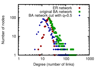
Figure 1: Degree distribution of unweighted ER network and BA network

The reason why we cut the links of BA networks randomly in step 2b is described below. According to the BA model [5], minimum degree $k_{\mathrm{min}}$ and average degree $k_{\mathrm{ave}}$ of original BA networks are always the same value when keeping the configuration of $n_{0}$ and $n_{a}$. On the contrary, $k_{\mathrm{min}}$ and $k_{\mathrm{ave}}$ of ER networks are randomly changed when keeping the configuration of $p$. By cutting the links of BA networks randomly, the BA networks have different $k_{\mathrm{min}}$ and $k_{\mathrm{ave}}$, and we can compare the results for BA networks and ER networks under comparable condition.

III-B The Universality and its Applicable Condition

We experimentally investigate the eigenvalue frequency distribution $f_{N}(\lambda)$ of normalized Laplacian matrix $\bm{N}$ for the randomly-weighted random networks, and clarify the universality (the Wigner semicircle law) of $f_{N}(\lambda)$ and the applicable condition.

In the investigation, we use the constant distribution with $w_{ij}=\overline{w}$, the uniform distribution with the range $[\overline{w}/2,\,3\,\overline{w}/2]$ and exponential distribution with the average $\overline{w}$ to set link weight $w_{ij}$ randomly. Note that these distributions have the same average of link weights, but a different variance of link weights. By the comparison of the results for the different distributions, we clarify the universality regardless of link weights in social networks. We repeat the generation of $\bm{N}$ 100 times, and calculate the average of these results. We use the parameter configuration shown in Tab. I as default.

TABLE I: Default parameter configuration

parameter	symbol	configuration
number of nodes	$n$	1,000
distribution of link weight $w_{ij}$		uniform distribution
average of link weights	$\overline{w}$	1
number of bins in $f_{N}(\lambda)$	$n_{h}$	50

We discuss the applicable condition of the universality on the basis of $k^{2}_{\mathrm{min}}$ and $k_{\mathrm{ave}}$ like the existing study [10]. In Fig. 2, we first show $k^{2}_{\mathrm{min}}$ and $k_{\mathrm{ave}}$ in randomly-weighted ER and BA networks with different expected average number of links, $k_{\rm ave}$, and the uniform distribution. As $k_{\rm ave}$ increases, $k^{2}_{\mathrm{min}}$ and $k_{\mathrm{ave}}$ increases simultaneously, but the increasing speed of $k^{2}_{\mathrm{min}}$ is larger than that of $k_{\mathrm{ave}}$. According to Fig. 2, in order to fulfill the degree condition $k^{2}_{\mathrm{min}}\gg k_{\mathrm{ave}}$ in [10], $k_{\mathrm{ave}}\geq 16$ for ER network and $k_{\mathrm{ave}}\geq 24$ for BA network are needed at least, respectively. In this paper, we set the average of link weight $w_{ij}$ to an amount equal to or greater than 1. Hence, if $k^{2}_{\mathrm{min}}\gg k_{\mathrm{ave}}$ is fulfilled, $d^{2}_{\mathrm{min}}\gg d_{\mathrm{ave}}$ is also fulfilled in average. Hence, we use $k^{2}_{\mathrm{min}}\gg k_{\mathrm{ave}}$ instead of $d^{2}_{\mathrm{min}}\gg d_{\mathrm{ave}}$ in order to clarify the applicable condition regardless of link weights.

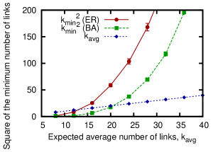
Figure 2: The expected average number $k_{\mathrm{ave}}$ of links vs. the square of the minimum number $k_{\mathrm{min}}$ of links in randomly-weighted ER network and BA network

In Figs. 3 and 4, we show eigenvalue frequency distributions $f_{N}(\lambda)$ of normalized Laplacian matrix $\bm{N}$ for randomly-weighted ER and BA networks, respectively. When we obtained $f_{N}(\lambda)$, we first counted the number of eigenvalues of $\bm{N}$ within $[\lambda-h_{b}/2,\lambda+h_{b}/2]$ where $h_{b}=(\lambda_{n}-\lambda_{2})/n_{h}$. Then, we normalized the counted number so that $\sum_{i=1}^{n_{h}}f_{N}(\theta_{i})=1$ where $\theta_{i}=\lambda_{2}+(i-1/2)\,h_{b}$, and $n_{h}$ is the number of bins in $f_{N}(\lambda)$. Note that we took out the minimum eigenvalue $\lambda_{1}$ of $\bm{N}$ when obtaining $f_{N}(\lambda)$ because $\lambda_{1}$ is always 0. In Figs. 3 and 4, we also draw the semicircle distribution, which is given by

$$\rho_{N}(\lambda)=\begin{cases}\displaystyle\frac{2}{\pi\,r^{2}}\sqrt{r^{2}-(\lambda-1)^{2}}&\!\!(\lambda_{2}<\lambda<\lambda_{n})\\ 0&\!\!(\mathrm{otherwise})\end{cases},$$ (7)

where $r$ is the radius of the semicircle distribution, and is given by $1-\lambda_{2}$ or $\lambda_{n}-1$. According to the range of $\lambda_{2}$ and $\lambda_{n}$, $r$ must be within $0<r<1$. Equation (7) is essentially equivalent to Eq. (6) in the Wigner semicircle law because there is just the difference of the semicircle center. Hence, we define that the Wigner semicircle law is satisfied if eigenvalue frequency distribution $f_{N}(\lambda)$ coincides with the semicircle distribution given by Eq. (7). According to Figs. 3 and 4, eigenvalue frequency distribution $f_{N}(\lambda)$ of $\bm{N}$ for the randomly-weighted ER and BA networks with $k_{\rm ave}=8$ differs from the semicircle distribution (7), but the distributions for the randomly-weighted ER and BA networks with $k_{\rm ave}=36$ almost coincide with it. Hence, we expect that large $k_{\rm ave}$ is needed to satisfy the Wigner semicircle law.

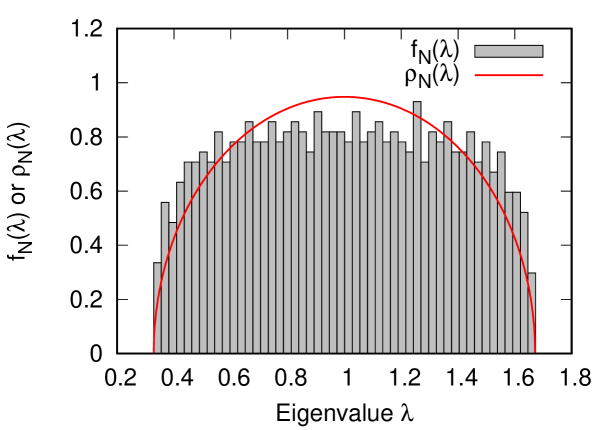
(a) $k_{\rm ave}=8$

(b) $k_{\rm ave}=36$

Figure 3: The eigenvalue frequency distributions of $\bm{N}$’s for randomly-weighted ER networks

(a) $k_{\rm ave}=8$

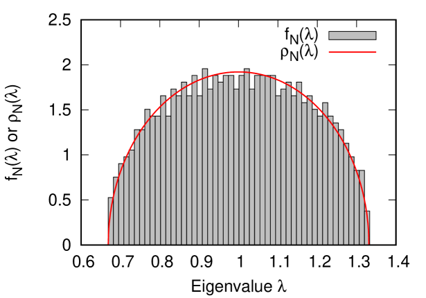
(b) $k_{\rm ave}=36$

Figure 4: The eigenvalue frequency distributions of $\bm{N}$’s for randomly-weighted BA networks

In order to clarify whether the eigenvalue frequency distribution $f_{N}(\lambda)$ satisfies the Wigner semicircle law, we investigate the difference between $f_{N}(\lambda)$ and $\rho_{N}(\lambda)$. As the definition of the difference, we use relative error $\epsilon$. Relative error $\epsilon$ is given by

$$\epsilon=\frac{1}{n_{h}}\sum_{i=1}^{n_{h}}\frac{|f_{N}(\theta_{i})-P(\theta_{i})|}{P(\theta_{i})},$$ (8)

where $\theta_{i}=\lambda_{2}+(i-1/2)\,h_{b}$, and $P(\theta_{i})$ is the probability that the eigenvalues of $\bm{N}$ is within $[\theta_{i}-h_{b}/2,\theta_{i}+h_{b}/2]$. Namely, $P(\theta_{i})$ is defined by

$$P(\theta_{i})=\int_{\theta_{i}-h_{b}/2}^{\theta_{i}+h_{b}/2}\rho_{N}(\lambda)\,\mathrm{d}\lambda.$$ (9)

Note that $P(\theta_{i})$ should become the true value of $f_{N}(\theta_{i})$ for $n\rightarrow\infty$ and $n_{h}\rightarrow\infty$.

In Fig. 5, we show the results of $\epsilon$ for randomly-weighted ER and BA networks with the constant distribution, the uniform distribution, and the exponential distribution of link weight $w_{ij}$. As $k_{\rm ave}$ increases, $\epsilon$ decreases regardless of the link weight distribution and network topology (ER or BA). The reason why $\epsilon$ does not approach to 0 is that there are discretization error due to the finite setting of $n$ and $n_{h}$. Moreover, $\epsilon$ for the uniform and exponential distributions approaches to that for the constant distribution. According to [10], $f_{N}(\lambda)$ with the constant distribution ($w_{ij}=1$) satisfies the Wigner semicircle law when the degree condition $k^{2}_{\mathrm{min}}\gg k_{\mathrm{ave}}$ is fulfilled. Hence, $f_{N}(\lambda)$ with the uniform and exponential distributions also satisfies the Wigner semicircle law.

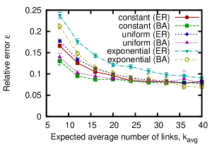
Figure 5: Relative error $\epsilon$ of eigenvalue frequency distribution $f_{N}(\lambda)$ for randomly-weighted ER and BA networks

From the above results, we can find that if the degree condition $k^{2}_{\mathrm{min}}\gg k_{\mathrm{ave}}$ is fulfilled, the eigenvalue frequency distribution of normalized Laplacian matrix $\bm{N}$ for randomly-weighted ER and BA networks satisfies the Wigner semicircle law given by Eq. (7), which is the semicircle distribution determined by only the second smallest eigenvalue $\lambda_{2}$ or the maximum eigenvalue $\lambda_{n}$ of $\bm{N}$. Hence, $\lambda_{2}$ and $\lambda_{n}$ are important to understand the social network property in the a case fulfilling the degree condition.

IV Analysis of the Information Propagation Speed

In this section, we analyze the speed of the information propagation on social networks fulfilling the degree condition $k^{2}_{\mathrm{min}}\gg k_{\mathrm{ave}}$. If the degree condition is not fulfilled in a social network, there are many persons with too small number of friends. However, such persons would be minority in an actual social network, and contribute less to the information propagation on the entire social network. Therefore, we ignore such persons, and focus on social networks fulfilling the degree condition.

IV-A Metric of the Information Propagation Speed

The information propagation in a social network is involved with the chain of word-of-mouth communications (e.g., face-to-face offline conversation, and online communication via SNS) between persons. In such a communication chain, the information is more likely to be propagated to the persons that have many friends. Random walks on a network have similar characteristic that the probability of the random walker arriving at a node is proportional to its node degree [11], which corresponds to the number of friends in a social network. Hence, we model the information propagation on social networks as a random walk. However, the information propagation modeled with the random walk may be too slower than the information propagation in an actual social network since the random walker arrives at the same node multiple times. Therefore, our analysis focuses on the worst-case situation for the information propagation in social networks.

Random walk on network $G$ is formulated by normalized Laplacian matrix $\bm{N}$. When node $i$ selects node $j$ with the probability $w_{ij}/d_{i}$, arrival probability $x_{a:i}(t)$ of the random walker starting from node $a$ to node $i$ at time $t$ is given by

$$x_{a:i}(t)=\sum_{j\in\partial i}\frac{w_{ji}}{d_{j}}x_{a:j}(t-1),$$ (10)

where $\partial i=\{j\ |\ A_{ij}>0,\ 1\leq j\leq n\}$. With arrival probability vector $\bm{x}_{a}(t)=(x_{a:i}(t))_{1\leq i\leq n}$, we obtain

$$\bm{x}_{a}(t) =\bm{x}_{a}(t-1)\bm{D}^{-1}\bm{A}$$

$$\bm{x}_{a}(t)\bm{D}^{-1/2} =\bm{x}_{a}(t-1)\bm{D}^{-1}\bm{A}\,\bm{D}^{-1/2}$$

$$\bm{y}_{a}(t) =\bm{y}_{a}(t-1)(\bm{I}-\bm{N}),$$ (11)

where $\bm{y}_{a}(t)=\bm{x}_{a}(t)\bm{D}^{-1/2}$.

A fundamental metric to evaluate of the information propagation speed in a social network is a first arrival time, which is the time required until the information is first propagated to a person. Such a first arrival time of the information corresponds to the time until the random walker first arrives at a node in the random walk. The existing study [11] derived first arrival time $f_{a:i}$ of the random walker starting from node $a$ to node $i$ as

$$f_{a:i}=2\,|E|\sum_{l=2}^{n}\frac{1}{\lambda_{l}}\left(\frac{q_{l}^{2}(i)}{d_{i}}-\frac{q_{l}(a)\,q_{l}(i)}{\sqrt{d_{a}\,d_{i}}}\right),$$ (12)

where $q_{l}(i)$ is the $i$-th element of eigenvector $\bm{q}_{l}$ of normalized Laplacian matrix $\bm{N}$. Since the steady-state probability of the random walk arriving at node $i$ is given by $d_{i}/(2\,|E|)$, expected value $m$ of first arrival time $f_{a:i}$ is derived as

$$m =\sum_{i=1}^{n}\frac{d_{i}}{2\,|E|}f_{a:i}$$

$$=\sum_{i=1}^{n}\sum_{l=2}^{n}\frac{1}{\lambda_{l}}\left(q_{l}^{2}(i)-\frac{q_{l}(a)\,q_{l}(i)}{\sqrt{d_{a}}}\,\sqrt{d_{i}}\right)$$

$$=\sum_{l=2}^{n}\frac{1}{\lambda_{l}}\left(\sum_{i=1}^{n}q_{l}^{2}(i)-\frac{q_{l}(a)}{\sqrt{d_{a}}}\sum_{i=1}^{n}q_{l}(i)\sqrt{d_{i}}\right)$$

$$=\sum_{l=2}^{n}\frac{1}{\lambda_{l}}\left(\sum_{i=1}^{n}q_{l}^{2}(i)-\frac{\sqrt{2\,|E|}\,q_{l}(a)}{\sqrt{d_{a}}}\sum_{i=1}^{n}q_{l}(i)\,q_{1}(i)\right)$$

$$=\sum_{l=2}^{n}\frac{1}{\lambda_{l}}.$$ (13)

When we derived the above equation, we used $q_{1}(i)=\sqrt{d_{i}/(2\,|E|)}$ and the property that $\bm{q}_{l}$ is the orthonormal basis. From the above equation, we find that $m$ can be calculated with only eigenvalue $\lambda_{l}$ of normalized Laplacian matrix $\bm{N}$, and does not depend on starting node $a$. In our analysis, we use $m$ as the information propagation metric of the social network.

IV-B The Information Propagation Speed with the Universality of Normalized Laplacian Matrix $\bm{N}$

Using the universality shown in Sect. III, we analyze the information propagation speed. According to the universality, eigenvalue frequency distribution $f_{N}(\lambda)$ of $\bm{N}$ for randomly-weighted networks is approximated by $\rho_{N}(\lambda)$, which given by Eq. (7). We first derive $\tilde{m}$ that is the approximated value of $m$ with the assumption that $f_{N}(\lambda)\simeq\rho_{N}(\lambda)$. Then, we discuss the information propagation speed on the basis of $\tilde{m}$.

If $f_{N}(\lambda)\simeq\rho_{N}(\lambda)$, expected value $m$ of first arrival time $f_{a:i}$ is approximated by

$$m =\sum_{l=2}^{n}\frac{1}{\lambda_{l}}\simeq(n-1)\sum_{i=1}^{n_{h}}\frac{1}{\theta_{i}}f_{N}(\theta_{i})$$

$$\simeq(n-1)\int_{\lambda_{2}}^{\lambda_{n}}\frac{1}{\lambda}\,\rho_{N}(\lambda)\,\mathrm{d}\lambda$$

$$=\frac{2\,(n-1)}{\pi\,r^{2}}\int_{\lambda_{2}}^{\lambda_{n}}\frac{1}{\lambda}\sqrt{r^{2}-(\lambda-1)^{2}}\,\mathrm{d}\lambda$$

$$=\frac{2\,(n-1)}{r^{2}}\left(1-\sqrt{1-r^{2}}\right)=\tilde{m},$$ (14)

where $\theta_{i}=\lambda_{2}+(i-1/2)\,h_{b}$ and $h_{b}=(\lambda_{n}-\lambda_{2})/2$. The detailed deviation process of Eq. (14) is provided in the appendix. According to Eq. (14), $\tilde{m}$ is only determined by the number $n$ of nodes, and radius $r$ of the semicircle distribution.

On the basis of Eq. (14), we analyze the worst-case speed of the information propagation in a social network. Figure 6 shows $\tilde{m}$ given by Eq. (14) as the function of radius $r$. Note that $r$ is within the range $(0,1)$ because $0<\lambda_{2},\lambda_{n}<2$. From this figure, $\tilde{m}$ is the monotonically increasing function of $r$ because of $\mathrm{d}\,\tilde{m}/\mathrm{d}\,r>0$ for $0<r<1$. Hence, if $m$ is able to be approximated by $\tilde{m}$, the worst-case speed of the information propagation in a social network becomes slower as $r$ increases. Moreover, since the range of $r$ is $0<r<1$, the lower bound and upper bound of $\tilde{m}$ are given by $n-1$ and $2\,(n-1)$, respectively. Hence, if the structure (i.e., relationship among people) of a social network changes, the worst-case speed of the information propagation changes at most 2.

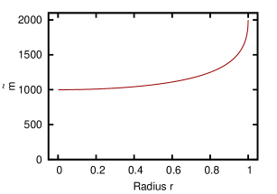
Figure 6: Radius $r$ vs. $\tilde{m}$

IV-C The Validity of Our Analysis

Our analysis is valid if the difference between $m$ and $\tilde{m}$ is sufficiently small. To investigate the difference, we use relative error $\epsilon_{m}$, which is defined by

$$\epsilon_{m}=\frac{|\tilde{m}-m|}{m}.$$ (15)

In the investigation, we repeat the generation of $\bm{N}$ 100 times, and calculate the average of related error $\epsilon_{m}$. Like Sect. III, we use the the parameter configuration shown in Tab. I as default, and randomly-weighted ER or BA networks. These networks have no cluster that is the set of densely-connected nodes, and is often observed in an actual social network. In general, the information propagation in a cluster is very fast, and so a cluster can be a node in the information propagation. Hence, the investigation with BA and ER networks is also valid for actual social networks, which may have clusters.

Figure 7 shows relative error $\epsilon_{m}$ for randomly-weighted ER and BA networks. According to this figure, $\epsilon_{m}$ approaches to 0 as $k_{\rm ave}$ increases regardless of the link weight distribution and network topology. Although the discretization error due to $n$ and $n_{h}$ affects relative error $\epsilon$ of eigenvalue frequent distribution $f_{N}(\lambda)$, it does not affect $\epsilon_{m}$. This characteristic is useful for the information propagation analysis.

By the comparison between Figs. 2 and 7, we conclude that our analysis based on Eq. (14) is valid for social networks if the degree condition $k^{2}_{\mathrm{min}}\gg k_{\mathrm{ave}}$ is fulfilled.

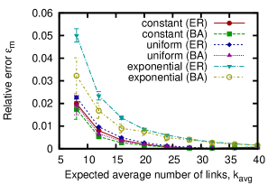
Figure 7: Relative error $\epsilon_{m}$ of expected value of first-arrival time $f_{a:i}$ for randomly-weighted ER and BA networks

V Conclusion and Future Work

Spectral graph theory cannot be simply applied to social network analysis because the matrix elements used in the theory cannot be given exactly to represent the structure of a social network. For this reason, we first discussed the universality of random matrix with the feature of social networks. As such random matrix, we used normalized Laplacian matrix $\bm{N}$ for a network where link weights are randomly given. We clarified that the universality (i.e., the Wigner semicircle law given by Eq. (7)) of normalized Laplacian matrix $\bm{N}$ appears regardless of the link weight distribution in ER networks and BA networks. According to the universality, eigenvalue frequency distribution $f_{N}(\lambda)$ of $\bm{N}$ is is determined by only the number $n$ of nodes and semicircle radius $r=1-\lambda_{2}$ or $\lambda_{n}-1$ where $\lambda_{2}$ and $\lambda_{n}$ are the second minimum eigenvalue and the maximum eigenvalue of $\bm{N}$, respectively. Then, we analyzed the information propagation speed in a social network on the basis of the spectral graph theory and the clarified universality. In this analysis, we modeled the information propagation by a random walk in the light of the resemblance between their characteristics, and investigated expected value $m$ of first arrival times of the random walker for each node. Our analysis showed that the worst-case speed of the information propagation changes at most 2 if the structure (i.e., relationship among people) of a social network changes.

As future work, we will investigate the relationship between topological property (e.g., scale-free property) and radius $r$ since $r$ determines the information propagation speed in a social network. Then, we are planning to design a social media for effective information propagation on the basis of the finding by our work.

Appendix

We describe the detailed deviation process of Eq. (14). If eigenvalue frequency distribution $f_{N}(\lambda)$ is given by the Wigner semicircle law, expected value $m$ of the first-arrival time is approximated by $\tilde{m}$. $\tilde{m}$ is given by

$$\tilde{m} =(n-1)\int_{\lambda_{2}}^{\lambda_{n}}\frac{1}{\lambda}\,\rho_{N}(\lambda)\,\mathrm{d}\lambda$$

$$=\frac{2\,(n-1)}{\pi\,r^{2}}\int_{\lambda_{2}}^{\lambda_{n}}\frac{1}{\lambda}\sqrt{r^{2}-(\lambda-1)^{2}}\,\mathrm{d}\lambda.$$ (A.1)

By substituting $\lambda=r\,\cos\theta+1$ into Eq. (A.1), we obtain

$$\tilde{m} =\frac{2\,(n-1)}{\pi\,r^{2}}\int_{0}^{\pi}\frac{r^{2}\,\sin^{2}\theta}{r\,\cos\theta+1}\,\mathrm{d}\theta$$

$$=\frac{2\,(n-1)}{\pi\,r^{2}}\int_{0}^{\pi}\frac{r^{2}-1+1-r^{2}\,\cos^{2}\theta}{r\,\cos\theta+1}\,\mathrm{d}\theta$$

$$=\frac{2\,(n-1)}{\pi\,r^{2}}\int_{0}^{\pi}\left(\frac{r^{2}-1}{r\,\cos\theta+1}+1-r\,\cos\theta\right)\,\mathrm{d}\theta$$

$$=I_{1}(r)+I_{2}(r),$$ (A.2)

where $I_{1}(r)$ and $I_{2}(r)$ are given by

$$I_{1}(r) =\frac{2\,(n-1)}{\pi\,r^{2}}\int_{0}^{\pi}\frac{r^{2}-1}{r\,\cos\theta+1}\,\mathrm{d}\theta,$$ (A.3)

$$l_{2}(r) =\frac{2\,(n-1)}{\pi\,r^{2}}\int_{0}^{\pi}\left(1-r\,\cos\theta\right)\,\mathrm{d}\theta,$$ (A.4)

respectively. When we use the half-angle formula of $\cos\theta$, $l_{1}(r)$ is given by

$$I_{1}(r) =\frac{2\,(n-1)}{\pi\,r^{2}}$$

$$\quad\times\int_{0}^{\pi}\frac{r^{2}-1}{r\left(\cos^{2}\frac{\theta}{2}-\sin^{2}\frac{\theta}{2}\right)+\left(\cos^{2}\frac{\theta}{2}+\sin^{2}\frac{\theta}{2}\right)}\,\mathrm{d}\theta$$

$$=\frac{2\,(n-1)}{\pi\,r^{2}}\int_{0}^{\pi}\frac{r^{2}-1}{(1+r)\,\cos^{2}\frac{\theta}{2}+(1-r)\,\sin^{2}\frac{\theta}{2}}\,\mathrm{d}\theta$$

$$=\frac{2\,(n-1)}{\pi\,r^{2}}\int_{0}^{\pi}\frac{r^{2}-1}{(1+r)+(1-r)\,\tan^{2}\frac{\theta}{2}}\frac{1}{\cos^{2}\frac{\theta}{2}}\,\mathrm{d}\theta$$

$$=\frac{2\,(n-1)}{\pi\,r^{2}}\int_{0}^{\pi}\frac{r-1}{1-\mathrm{i}^{2}\,\frac{1-r}{1+r}\,\tan^{2}\frac{\theta}{2}}\frac{1}{\cos^{2}\frac{\theta}{2}}\,\mathrm{d}\theta,$$ (A.5)

where $\mathrm{i}$ is the imaginary unit. By substituting $x=\sqrt{\frac{1-r}{1+r}}\tan\frac{\theta}{2}$ into Eq. (A.5), $l_{1}(r)$ is derived as

$$I_{1}(r) =\frac{2\,(n-1)}{\pi\,r^{2}}\int_{0}^{\infty}\frac{-2\,\sqrt{1-r^{2}}}{1-(\mathrm{i}\,x)^{2}}\,\mathrm{d}x$$

$$=\frac{2\,(n-1)}{\pi\,r^{2}}$$

$$\quad\times\int_{0}^{\infty}\left(-\sqrt{1-r^{2}}\right)\left(\frac{1}{1+\mathrm{i}\,x}+\frac{1}{1-\mathrm{i}\,x}\right)\,\mathrm{d}x$$

$$=\frac{2\,(n-1)}{\pi\,r^{2}}\left(-\sqrt{1-r^{2}}\right)$$

$$\quad\times\Bigl{[}\frac{1}{\mathrm{i}}\,\log(1+\mathrm{i}\,x)-\frac{1}{\mathrm{i}}\,\log(1-\mathrm{i}\,x)\Bigr{]}_{0}^{\infty}$$

$$=\frac{2\,(n-1)}{\pi\,r^{2}}\left(\mathrm{i}\,\sqrt{1-r^{2}}\right)$$

$$\quad\times\lim_{x\rightarrow\infty}\Bigl{[}\log(1+\mathrm{i}\,x)-\log(1-\mathrm{i}\,x)\Bigr{]}.$$ (A.6)

When we use $\log z=\log|z|+\mathrm{i}\,\mathrm{arg}(z)$, $I_{1}(r)$ is derived as

$$I_{1}(r) =\frac{2\,(n-1)}{\pi\,r^{2}}\left(\mathrm{i}\,\sqrt{1-r^{2}}\right)\lim_{x\rightarrow\infty}2\,\mathrm{i}\,\tan^{-1}x$$

$$=-\frac{2\,(n-1)}{r^{2}}\sqrt{1-r^{2}}.$$ (A.7)

Then, $l_{2}(r)$ is derived as

$$I_{2}(r) =\frac{2\,(n-1)}{\pi\,r^{2}}\int_{0}^{\pi}\left(1-r\,\cos\theta\right)\,\mathrm{d}\theta$$

$$=\frac{2\,(n-1)}{\pi\,r^{2}}\Bigl{[}\theta-r\,\sin\theta\Bigr{]}_{0}^{\pi}$$

$$=\frac{2\,(n-1)}{r^{2}}.$$ (A.8)

By substituting Eqs. (A.7) and (A.8) into Eq. (A.2), $\tilde{m}$ is given as

$$\tilde{m} =I_{1}(r)+I_{2}(r)$$

$$=\frac{2\,(n-1)}{r^{2}}\left(1-\sqrt{1-r^{2}}\right).$$ (A.9)

References

- [1] F. Chung, Spectral Graph Theory. American Mathematical Society, 1997.
- [2] T. Guhr, A. Müller-Groeling, and H. A. Weidenmüller, “Random-matrix theories in quantum physics: common concepts,” Physics Reports, vol. 299, pp. 189–425, June 1998.
- [3] E. P. Wigner, “On the distribution of the roots of certain symmetric matrices,” Annals of Mathematics, vol. 67, no. 2, pp. 325–327, 1958.
- [4] P. Erdös and A. Rényi, “On random graphs,” Mathematicae, vol. 6, no. 26, pp. 290–297, 1959.
- [5] A. L. Bárabasi and R. Albert, “Emergence of scaling in random networks,” Science, vol. 286, pp. 509–512, Oct. 1999.
- [6] C. Zhan, G. Chen, and L. F. Yeung, “On the distributions of laplacian eigenvalues versus node degrees in complex networks,” Physica A: Statistical Mechanics and its Applications, vol. 389, pp. 1779–1788, Apr. 2010.
- [7] S. Jalan and J. N. Bandyopadhyay, “Random matrix analysis of network laplacians,” Physica A: Statistical Mechanics and its Applications, vol. 387, pp. 667–674, Jan. 2008.
- [8] I. J. Farkas, I. Derényi, A.-L. Barabási, and T. Vicsek, “Spectra of “real-world” graphs: Beyond the semicircle law,” Physical Review E, vol. 64, p. 026704, July 2001.
- [9] Y. Sakumoto and H. Ohsaki, “Fluid-based analysis for understanding tcp performance on scale-free structure,” Journal of Information Processing, vol. 24, pp. 660–668, July 2016.
- [10] F. Chung, L. Lu, and V. Vu, “Spectra of random graphs with given expected degrees,” Proceedings of the National Academy of Sciences, vol. 100, pp. 6313–6318, May 2003.
- [11] L. Lovász, “Random walks on graphs: a survey,” Combinatorics, Paul Erdős is eighty, vol. 2, pp. 353–398, 1996.