Quantum Tunneling Of Electron Snake States In An Inhomogeneous Magnetic Field

Abstract

In a two dimensional free electron gas (2DEG) subjected to a perpendicular spatially varying magnetic field, the classical paths of electrons are snake-like trajectories that weave along the line where the field crosses zero. But quantum mechanically this system is described by a symmetric double well potential which, for low excitations, leads to very different electron behavior. We compute the spectrum, as well as the wavefunctions, for states of definite parity in the limit of nearly degenerate states, i.e. for electrons sufficiently far from the $B_{z}=0$ line. Transitions between the states are shown to give rise to a tunneling current. If the well is made asymmetrical by a time-dependent parity breaking perturbation then Rabi-like oscillations between parity states occur. Resonances can be excited and used to stimulate the transfer of electrons from one side of the potential barrier to the other through quantum tunneling.

To be published in Journal of Physics:Condensed Matter

Snake orbitals exist in mesoscopic systems where electrons may be presumed to move freely in a two-dimensional electron gas (2-DEG) such as created by using a GaAs/GaAlAs heterostructure. If such a system is subjected to a perpendicular magnetic field whose strength varies linearly from one edge of the sample to the other then, classically speaking, an electron moving close to the line where $B_{z}=0$ alternately experiences regions of oppositely directed fields and so the Lorentz force redirects trajectories towards this boundary. In what becomes effectively a 1-D magnetic quantum wire, electrons can propagate unidirectionally in snake-like fashion. The first quantum calculation of electron trajectories and the energy spectrum of such a system was carried out by Muller Muller . This involved numerical diagonalization of the Hamiltonian in a harmonic oscillator basis. Using qualitative reasoning, he pointed out that snake states weaving around the $B_{z}=0$ boundary break time reversal symmetry in the sense that electrons close to the boundary can propagate as free particles in one direction but not in the other. Following up on Muller’s calculation, Reijniers and coworkers Reijners1 Reijners2 performed extensive numerical calculations and were able to give a clearer picture of such states, including their confinement due to interference between oppositely directed waves. However those calculations were done in a model that is somewhat unrealistic, i.e. one in which the magnetic field increases by a discrete step.

Calculations in inhomogeneous fields assume relevance because studying electron motion in appropriate mesoscopic situations has been well within experimental grasp for many years now. Nogaret Nogaret has reviewed electron dynamics in inhomogeneous fields and experimental strategies for making such fields. Recent technological advances have allowed the fabrication of high mobility 2-DEGs with nanomagnets of well defined shapes placed above or below, allowing one to study the effect of inhomogeneous $B$ fields with different profiles. These distributions can profoundly influence electron transport properties and may lead towards the design of useful magnetoelectronic devices. Using the idea of classical snake states one may compute, for example, the magnetoresistance of such systems Rectification - only to discover that this picture of electron motion becomes progressively incorrect as $B$ is increased and the electron density decreased. Quantum effects become more pronounced in these situations. This phenomenon has been observed by Schuler et. al Expt2 who studied resonant transmission through electronic quantum states that exist at the zero points inside a ballistic quantum wire. They explored the dependence on the amplitude of the magnetic field as well as on the Fermi energy. Maha et. al Expt1 have observed asymmetric transport and rectification effects associated with snake states.

The present paper examines the nature of snake states in a region where quantum properties are dominant and semi-classical arguments become inapplicable. The goal is to make as much progress analytically as possible; while numerical calculations are often essential, one pays the price of decreased intuition. In the case under consideration, although one cannot fully succeed in achieving closed form solutions, some progress can be made by invoking ideas familiar from WKB theory and instanton methods.

The specific situation considered here is as in ref Muller , i.e. a magnetic field is directed perpendicularly to a 2-DEG that varies linearly in strength from one edge of the sample to the other. Electrons in Landau levels on opposite sides of the $B_{z}=0$ boundary have identical energies if the Zeeman coupling is ignored. This degeneracy results in tunneling across a potential barrier. The consequence is a current transverse to the field gradient. States of opposite parity are shown to carry currents in opposite directions. We show that if an additional external time-varying electric field of appropriate frequency is imposed, Rabi-like oscillations occur and these can be used to identify the orbital centers of the tunneling electrons. This mechanism allows electrons in Landau orbits to swap positions across the $B_{z}=0$ line.

I Preliminaries

Our starting point is the 2-D Schrödinger equation describing free electrons confined to a rectangular $(L_{x},L_{y})$ sample. A $\hat{z}$-directed magnetic field increases linearly with $y$, $\ \vec{B}(y)=(0,0,yB^{\prime})$. The origin of coordinates will be taken to be at the sample’s centre. The Hamiltonian is,

$$H=\frac{1}{2m}\left(\mathbf{p}-\frac{e}{c}\mathbf{A}\right)^{2}.$$ (1)

The gauge potential is chosen as,

$$\mathbf{A=}-\hat{x}\frac{1}{2}y^{2}B^{\prime}.$$ (2)

This potential is translationally invariant in $x$. This implies a plane wave solution, $\psi(x,y)=\frac{1}{\sqrt{L_{x}}}e^{-ik_{x}x}\varphi(y)$. It is convenient to define a relevant magnetic length scale $L_{M},$

$$L_{M}=\left(\frac{2\hslash c}{eB^{\prime}}\right)^{1/3}.$$ (3)

After rescaling, $\varphi$ satisfies a reduced eigenvalue equation with the single parameter $\alpha,$

$$\left(-\frac{1}{2}\frac{d^{2}}{d\eta^{2}}+V(\eta)\right)\varphi=\epsilon\varphi\,,\text{ }V(\eta)=\frac{1}{2}(\eta^{2}-\alpha^{2})^{2}\,.$$ (4)

In the above,

$$\eta=\frac{y}{L_{M}},\text{ \ }\alpha^{2}=k_{x}L_{M},\text{ \ }E=\frac{\hslash^{2}}{mL_{M}^{2}}\epsilon.$$ (5)

The quantity $k_{x}$ is the eigenvalue of $\hat{p}_{x}=$ $\frac{\hslash}{i}\frac{\partial}{\partial x}$. One notes that $\hat{p}_{x}$ is not the canonical momentum operator and so $k_{x}$ is unrelated to the physical momentum. Translational invariance in $x$ allows periodic boundary conditions $\psi(x+L_{x},y)=\psi(x,y)$ to be imposed. The sum over $k_{x}$ (which, of course, can take either sign) can therefore be converted to an integral,

$$\ \sum_{k_{x}}\longrightarrow\frac{L_{x}}{2\pi}\int dk_{x}\ =\frac{1}{\pi}\frac{L_{x}}{L_{M}}\int\alpha d\alpha.$$ (6)

The sum over $k_{x}$ means that we shall have to deal with values of $\alpha^{2}$ that can take both positive and negative values. In the case $k_{x}>0$ there are minima of the potential located at $\eta=\pm\alpha$. On the other hand, for $k_{x}<0$ the two minima coalesce at $\eta=0.$  The eigenfunctions for the two cases also, of course, have qualitatively different behaviors.

The double well oscillator of Eq.4 is famously unsolvable and has no exact solutions. But this seemingly simple potential actually has rich structure and has been pursued because it occurs in quantum field theory as well as various branches of physics and molecular chemistry. In fact it has been the subject of nearly a thousand investigations, many of which have followed the pioneering work of Bender and Wu Bender1 -Bender2 . Of course, one can always seek approximate solutions. In the limit of large negative $\alpha^{2}$ the eigenvalues are easily found to be,

$$\epsilon_{n}=\frac{1}{2}\alpha^{4}+\left(n+\frac{1}{2}\right)\sqrt{2\left|\alpha^{2}\right|},$$ (7)

or, upon restoring units,

$$E_{n}=\frac{\hslash^{2}k_{x}^{2}}{2m}+\left(n+\frac{1}{2}\right)\sqrt{\frac{e\hslash^{3}B^{\prime}}{m^{2}c}\left|k_{x}\right|},$$

The lowest eigenvalues of Eq.4 are also easily obtained in the limit of large positive $\alpha^{2}.$ These correspond to the two minima being widely separated although, for now, we do not know what this means in quantitative terms. Intuitively it should mean the absence of appreciable tunneling between the well minima because of the intervening high potential barrier whose maximum is $V(0)=\frac{1}{2}\alpha^{4}$. In this situation the double well potential can be harmonically approximated by two single isolated wells, $V(\eta)=\frac{1}{2}(2\alpha)^{2}(\eta\pm\alpha)^{2}$ with $2\alpha$ being the classical oscillation frequency. The normalized eigenfunctions are the usual Hermite polynomials,

$$\frac{1}{\sqrt{2^{n}n!}}\left(\frac{2\alpha}{\pi}\right)^{1/4}H_{n}[\sqrt{2\alpha}(\eta\pm\alpha)]e^{-\alpha(\eta\pm\alpha)^{2}},$$ (8)

that correspond to the energy,

$$\epsilon_{n,\alpha,\pm}=2\alpha\left(n+\frac{1}{2}\right).$$ (9)

In this extreme asymptotic limit the eigenstates are degenerate and may be chosen to have definite parity,

$$\varphi_{n}^{\pm}(\eta)=\frac{1}{\sqrt{2}}\left[\varphi_{n}(\eta-\alpha)\pm\varphi_{n}(\eta+\alpha)\right].$$ (10)

Note that the energy of a gyrating electron increases linearly with $\alpha,$ i.e. in either direction from the sample’s centre. This is in contrast to the case of a uniform field where the energy is flat and Landau levels of a given $n$ are massively degenerate.

By expanding in a harmonic oscillator basis, one can numerically diagonalize the Hamiltonian in Eq.4. In Fig.1 the lowest few eigenvalues are plotted as a function of $\alpha^{2}$ for both signs of $\alpha^{2}$. One can see the emergence of a band structure. The asymptotic conditions leading to Eq.7 and Eq.9  are well satisfied. The confining walls can be chosen far enough away so as to have negligible influence upon the wavefunctions on the $y=0$ line.

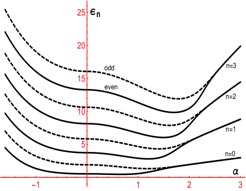
Figure 1: Energies of the lowest electron states obtained through numerical diagonalization. Lower/upper curves for a given $n$ are of even/odd parity. These are plotted as a function of $\alpha,$ with $\alpha^{2}>0$ towards the right and $\alpha^{2}<0$ on the left.

Consider now the interval of $\alpha$ where an electron is almost, but not wholly, confined to the two well minima. If one is originally centred at $\eta=\alpha$, it will bounce within the confines of its own well but will occasionally manage to tunnel across to the other well at $\eta=-\alpha$ before returning after some finite time. For larger $\alpha^{\prime}s,$ i.e larger separation between the two minima, tunneling will become less frequent. Note that $\alpha^{-1}$ plays the role of $\hslash$ in the usual quantum double oscillator, the smallness of which is crucial to the success of semi-classical methods. These methods are essential because non-analyticity in the coupling constant makes perturbation theory useless. Over the years, in a tour de force, Zinn-Justin and collaborators Zinn1 -Zinn2 have used sophisticated resurgent trans-series techniques involving a leading-order summation of multi-instanton contributions to the path integral representation of the partition function for calculating corrections to the leading order result for eigenvalues. After appropriately scaling their results to the present case, the first few terms for $n=0$ and $n=1$ are:

$$\epsilon_{0,\pm} = \alpha\mp\frac{1}{\sqrt{\pi}}2^{\frac{5}{2}}\alpha^{\frac{5}{2}}e^{-\frac{4\alpha^{3}}{3}}$$ (11)

$$\times\left(1-\frac{71}{96\alpha^{3}}-\frac{6299}{18432\alpha^{6}}-\frac{2691107}{5308416\alpha^{9}}\right)$$

$$\epsilon_{1,\pm} = 3\alpha\mp\frac{1}{\sqrt{\pi}}2^{\frac{13}{2}}\alpha^{\frac{11}{2}}e^{-\frac{4\alpha^{3}}{3}}$$ (12)

$$\times\left(1-\frac{347}{96\alpha^{3}}+\frac{5317}{18432\alpha^{6}}-\frac{15995159}{5308416\alpha^{9}}\right)$$

To be added to the above are parity independent terms whose first 300, 70 terms for $n=0,1$ respectively have been calculated by the authors in perturbation theory. These shall not be of interest here, but we shall use in Fig.2 the correction factors in the brackets above.

II Wavefunctions

We now consider electrons orbiting around gyration centres located at $\pm\alpha$. The Hamiltonian Eq.4 is even under $\eta\rightarrow-\eta$ so one can restrict attention to the region $\eta\geq 0$. We follow the philosophy of ColemanColeman by insisting that the solution inside a well centred at $\alpha$ be well approximated by a wavefunction close to that of a SHO. For energies sufficiently below the well maximum $\alpha^{4}/2$, tunneling splits the ground state’s degeneracy by a small amount proportional to $\delta$ with $\delta>0.$ The positive parity state, by virtue of having smaller curvature (less kinetic energy), has lower energy,

$$\epsilon_{n\pm}=\left(n+\frac{1}{2}\right)2\alpha(1\mp\delta),\text{ \ }\alpha^{3}>>2\left(2n+1\right).\text{\ }$$ (13)

Here $n$ is a non-negative integer. Near the well minimum $\eta=\alpha$ the potential is quadratic and for the positive parity state Eq.4 becomes,

$$-\frac{1}{2}\frac{d^{2}\Phi_{\pm}}{d\eta^{2}}+\frac{1}{2}4\alpha^{2}(\eta-\alpha)^{2}\Phi_{\pm}=\epsilon_{n\pm}\Phi_{\pm}\,.$$ (14)

To take the analysis further, let us define a new variable $z$ and rescaled energy $\epsilon$,

$$z = 2\sqrt{\alpha}(\eta-\alpha)$$

$$\varepsilon_{n\pm} = \frac{\epsilon_{n\pm}}{2\alpha}.$$

Temporarily suppressing the indices for clarity, this allows Eq.14 to be more simply written as,

$$\left(-\frac{d^{2}}{dz^{2}}+\frac{1}{4}z^{2}-\varepsilon\right)\Phi=0\,,$$ (15)

the solutions of which are the parabolic cylinder functions,

$$\Phi(z)=c_{1}D_{\varepsilon-\frac{1}{2}}(z)+c_{2}D_{-\varepsilon-\frac{1}{2}}(iz).$$ (16)

We first consider solutions for $z>0$. If the confining walls of the sample are sufficiently far away, then the second term must be discarded because for large positive $z$ this goes as $e^{z^{2}/4}$ and so we must choose $c_{2}=0$. Thus the wavefunction around the well minimum is,

$$\Phi(z)=N_{\varepsilon}D_{\varepsilon-\frac{1}{2}}(z),$$ (17)

where $N_{\varepsilon}$ is a normalization factor. Recalling that $\varepsilon_{n\pm}=(n+\frac{1}{2})(1\mp\delta)$ where $n$ is an integer, we recall that for $\delta=0$ the parabolic cylinder functions can be expressed in terms of the Hermite polynomials,

$$D_{n}(z)=2^{-\frac{n}{2}}H_{n}(z/\sqrt{2})e^{-z^{2}/4}.$$

To the left of the well minimum (i.e. $\eta<\alpha$ ) $D_{\varepsilon-\frac{1}{2}}\left(z\right)$ blows up as $z\rightarrow-\infty$. However the domain is actually finite, i.e. $z>-2\alpha^{3/2}$. To leading order in $\delta$ the asymptotic behavior in this region is,

$$\Phi_{n\pm}(z)=N_{n\pm}\left(z^{n}e^{-\frac{z^{2}}{4}}+\frac{\left(-1\right)^{n+1}\sqrt{2\pi}}{\Gamma[-n\pm(n+\frac{1}{2})\delta]}\frac{e^{\frac{z^{2}}{4}}}{z^{n+1}}\right).$$ (18)

For small $\delta$ the gamma function is

$$\Gamma[-n\pm(n+\frac{1}{2})\delta]=\pm\frac{\left(-1\right)^{n}}{n!}\frac{1}{(n+\frac{1}{2})\delta}+O(\delta^{0}),$$

and therefore the wavefunction for widely separated wells and fixed negative $z$ is, to leading order,

$$\Phi_{\pm}(z)=N_{n\pm}\left(z^{n}e^{-\frac{z^{2}}{4}}\mp\delta\sqrt{2\pi}(n+\frac{1}{2})n!\frac{e^{\frac{z^{2}}{4}}}{z^{n+1}}\right),\text{ }\ z<0.$$ (19)

We now have the parts of the wavefunction to the right and left of the well minimum. However Eq.19 evidently does not have the correct parity behavior under $\eta$ $\rightarrow$ $-$$\eta$, i.e. these approximate solutions do not obey $\varphi_{+}^{\prime}(0)$ $=0$ and $\varphi_{-}(0)$ $=0$. Hence we must return to Eq.4 and construct appropriate solutions near $\eta=0.$ We therefore look for solutions in the presence of the full quartic potential (i.e. solve Eq.4 rather than just the quadratic approximation to it). Inspired by the WKB method but independent of it, let us make the ansatz:

$$h(\eta)e^{-\alpha^{2}\eta+\frac{1}{3}\eta^{3}},$$ (20)

with $h(\eta)$ a function to be determined. Substituting into Eq.4 yields, to leading order in $\delta$,

$$h^{\prime\prime}-2(\alpha^{2}-\eta^{2})h^{\prime}+2(\alpha+2\alpha n+\eta)h=0.$$ (21)

For large $\alpha$ we can ignore the first term and obtain a first order equation that is immediately solvable,

$$h(\eta)=\frac{(\eta+\alpha)^{n}}{(\eta-\alpha)^{n+1}}$$

Since Eq.4 is even under $\eta\longleftrightarrow-\eta$ it follows that $h(-\eta)e^{\alpha^{2}\eta-\frac{1}{3}\eta^{3}}$ is equally well a solution. We may therefore form combinations of definite parity which, up to a multiplicative constant, for $0<\eta<\alpha$ are,

$$\Psi_{\pm}(\eta)\sim\frac{(\eta-\alpha)^{n}}{(\eta+\alpha)^{n+1}}e^{\alpha^{2}\eta-\frac{1}{3}\eta^{3}}\mp\frac{(\eta+\alpha)^{n}}{(\eta-\alpha)^{n+1}}e^{-\alpha^{2}\eta+\frac{1}{3}\eta^{3}},\text{ \ \ }$$ (22)

Transforming to the $z$ variable, $z=2\sqrt{\alpha}(\eta-\alpha)$ and taking the large $\alpha$ limit gives for $z>-2\alpha^{3/2}$,

$$\Psi_{\pm}(z)\rightarrow N_{\pm}\left[z^{n}e^{-\frac{z^{2}}{4}}\mp e^{-\frac{4}{3}\alpha^{3}}2^{4n+2}\alpha^{3(n+\frac{1}{2})}\frac{e^{\frac{z^{2}}{4}}}{z^{n+1}}\right],\text{ \ }.$$ (23)

Comparing Eq.23 with Eq.19, we see they can be matched provided,

$$\delta_{n}(\alpha) = \frac{2^{4n+\frac{3}{2}}\alpha^{3(n+\frac{1}{2})}}{\sqrt{\pi}(n+\frac{1}{2})n!}e^{-\frac{4}{3}\alpha^{3}}$$ (24)

$$N_{\pm} = N_{n\pm}$$ (25)

Quite remarkably the energy splittings obtained here are precisely those obtained in the one-instanton approximation. The extremely rapid decrease of $e^{-\frac{4}{3}\alpha^{3}}$ guarantees that $\delta_{n}(\alpha)$ will approach the true value for large enough $\alpha.$ In Fig.2 we compare the leading order result obtained above with the corrections shown in Eq.11-Eq.12.

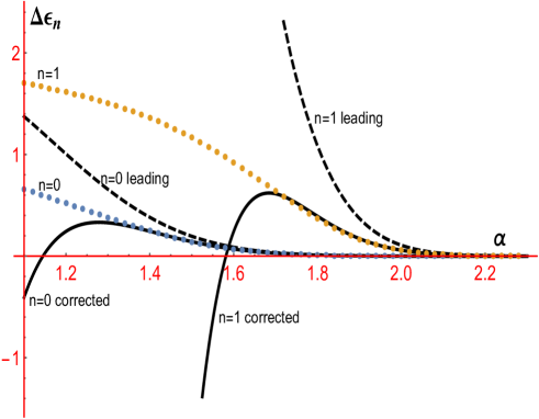
Figure 2: The energy difference between odd and even states as a function of $\alpha$ for $n=0,1$. Results obtained by numerical diagonalization (dotted) are compared against the leading order result as well as with those with multi-instanton corrections.

At this point we need to be more explicit about the domains in which different pieces of the wavefunction are valid. The wavefunction $D_{\varepsilon-\frac{1}{2}}(z)$ , in Eq.19 is valid around $z=0$ but not around $\eta=0$. On the other hand $\Psi_{\pm}\left(z\right)$ in Eq.23 has the correct behavior around $\eta=0$ but fails progressively as one approaches the well bottom. At which point should they be matched? There is clearly some ambiguity here but an obvious choice is the classical turning point to the left of $\alpha,$ i.e. when the potential energy in Eq.14 becomes equal to the eigenvalues, $2\alpha^{2}(\eta-\alpha)^{2}=\left(n+\frac{1}{2}\right)2\alpha.$ This gives the two turning points in the right plane,

$$z_{\pm}=\pm\sqrt{2(2n+1)}.$$

The final form of the wavefunction is,

$$\varphi_{n,\pm}(z)=\left\{\begin{array}[]{lr}\Psi_{\pm}(z):&-2\alpha^{3/2}<z<-\sqrt{2(2n+1)}\\ \Phi_{\pm}(z):&-\sqrt{2(2n+1)}<z<\infty\end{array}\right.$$

where $\Psi_{\pm}(z),\Phi_{\pm}(z)$ are defined in Eq.23, Eq.17 respectively.

III Tunneling Current

The important observable is the electron current $J_{x}$, or equivalently, the velocity v_x. The corresponding operator is obtained from the canonical momentum,

$$\text{\^{v}}_{x} = \frac{\mathbf{p}_{x}-\frac{e}{c}\mathbf{A}_{x}}{m}\,$$ (26)

$$= \frac{\hslash}{mL_{M}}(\eta^{2}-\alpha^{2})=\frac{\hslash}{mL_{M}}\left(\frac{z^{2}}{4\sqrt{\alpha}}+z\sqrt{\alpha}\right).$$

In the limit of large well separations $\alpha>>\left(n+\frac{1}{2}\right)^{1/3}$ the leading parity dependent contributions to the transverse current of an electron state centred at $\alpha$ is,

$$j_{x}^{\pm} = e\left\langle n,\alpha,\pm\left|\text{\^{v}}_{x}\right|n,\alpha,\pm\right\rangle$$ (27)

$$= \frac{e\hslash}{mL_{M}}\left[J_{n,\alpha}\mp\sqrt{\frac{9\pi}{2}}n!(n+\frac{1}{2})\alpha^{2}\delta_{n}(\alpha)\right].$$

Here $J_{n,\alpha}$ is the part of the current that is parity independent. While it is easy to get expressions for it, they cannot be evaluated analytically and integrations will have to be done numerically. Note that if both parity states are occupied then the oppositely directed currents cancel and so, if the current is to be detected, the Fermi level must be tuned (perhaps by varying an external electric potential) so that the last positive parity occupied state lies just below its negative parity partner. The y-directed current is obviously zero when evaluated in a parity eigenstate, $\left\langle\pm\left|\text{\^{v}}_{y}\right|\pm\right\rangle=0$.

The part of the current in Eq.27 that is proportional to $\delta_{n}(\alpha)$ owes entirely to $\Psi_{\pm}(z).$  The contribution of $\Phi_{\pm}(z)$ to this part is ignorable because it is of order $\alpha^{0}.$ It is easy to see why: continuity of $D_{\varepsilon-\frac{1}{2}}$ as a function of $\varepsilon$ means that any definite integral of the type $\int z^{\beta}\left|D_{\varepsilon-\frac{1}{2}}(z)\right|^{2}dz$ that is convergent changes linearly with $\varepsilon$, and hence linearly with $\delta_{n}(\alpha)$ as well. On the other hand, as can be seen in Eq.27 the dominant contribution to the parity sensitive terms is of order $\alpha^{2}\delta_{n}(\alpha).$ We see that the ambiguity in determining the matching point of the wavefunctions does not affect the leading order result. Since $\ e^{-\frac{4}{3}\alpha^{3}}$ decreases extremely fast with $\alpha$, we are essentially looking at the quantum properties of states that lie close to the line of zero $B$ field.

Let us return to physical considerations: an electron that is mostly on the right ($y>0$) is in a mixture of parity states $\left[\varphi_{+}(\eta)+\varphi_{-}(\eta)\right]/\sqrt{2}$ whereas an electron on the left has wavefunction $\left[\varphi_{+}(\eta)-\varphi_{-}(\eta)\right]/\sqrt{2}.$ If an electron swaps its position from right to left, the net change in the current it carries is easily seen to be,

$$\Delta j = \frac{e\hslash}{mL_{M}}\sqrt{\frac{9\pi}{2}}(n+\frac{1}{2})n!\alpha^{2}\delta_{n}(\alpha)$$ (28)

$$= \frac{e\hslash}{mL_{M}}6\alpha^{\frac{7}{2}}e^{-\frac{4}{3}\alpha^{3}}\text{ \ (for }n=0\text{).}\vskip 12.0pt plus 4.0pt minus 4.0pt$$ (29)

Consider an electron initially on the right that, for example, is in the $n=0$ state. It will will return to its original state after a time $\tau=2\pi\hslash/\Delta E$ where $\Delta E$ is the energy splitting $\frac{\hslash^{2}}{mL_{M}^{2}}2\alpha\delta_{0}(\alpha).$ Of course, no net current will have flowed since the going and returning current will have canceled over a complete cycle. How then are we to actually probe such states using the expession in Eq.28? This is taken up in the next section.

IV Time Dependent Field

The symmetric potential $V(\eta)$ in Eq. 1 has zeros at $\eta=\pm\alpha.$ Imagine introducing a small time-dependent symmetry breaking term proportional to $\eta$ or $\eta^{3}$, i.e. somehow rocking this potential so that one minimum sometimes lies slightly below the other. If this rocking frequency can be made to coincide with the natural time for a particle to tunnel across the potential and back, then we can expect an enhancement for electrons at a certain distance from the $B=0$ line, i.e. those at a particular value of $\alpha$. One way of achieving this might be to apply a weak oscillating electric field in the $\hat{y}$ direction. To this end, let us add a perturbing term to the Hamiltonian Eq.1. The time dependent Schrodinger equation is,

$$\left(-\frac{1}{2}\frac{\partial^{2}}{\partial\eta^{2}}+V(\eta)-\eta a_{E}\cos\omega_{E}\tau\right)\Phi=i\frac{\partial}{\partial\tau}\Phi$$ (30)

The dimensionless time is $\tau=\omega_{B}t$ where,

$$\omega_{B}=\frac{\hslash}{mL_{M}^{2}}$$ (31)

and $\omega_{E}$ is the applied frequency in units of $\omega_{B}$. The dimensionless amplitude of the applied field is,

$$\text{\ }a_{E}=\frac{2mc}{\hslash B^{\prime}}E_{y}.$$ (32)

If we choose only small amplitudes $a_{E}$ there will be negligible mixing with higher $n$ levels in which case it should be sufficient to confine ourselves to a two-dimensional space,

$$\Phi=\beta_{+}(\tau)e^{-i\varepsilon_{+}\tau}\varphi_{n+}(\eta)+\beta_{-}(\tau)e^{-i\varepsilon_{-}\tau}\varphi_{n-}(\eta).$$ (33)

Although the eigenfunctions and eigenvalues have been derived for arbitrary $n$, only the lowest values of $n$ are likely to be relevant. To avoid notational clutter, let us therefore specialize to $n=0$. The equations for the amplitudes $\beta_{\pm}$ follow straightforwardly from Eq.30,

$$i\text{ }\dot{\beta}_{+} = -a_{E}\alpha\beta_{-}e^{-i\omega_{D}\tau}\cos\omega_{E}\tau$$ (34)

$$i\text{ }\dot{\beta}_{-} = -a_{E}\alpha\beta_{+}e^{i\omega_{D}\tau}\cos\omega_{E}\tau$$ (35)

Here the difference frequency $\omega_{D}$ is,

$$\omega_{D} = \varepsilon_{-}-\varepsilon_{+}$$ (36)

$$= 8\sqrt{\frac{2\alpha^{5}}{\pi}}e^{-\frac{4\alpha^{3}}{3}}.$$ (37)

The coupled equations are essentially those of the well-known Rabi oscillations. Eqs.34-35 can be solved in the well known rotating wave approximation Fujii . This amounts to replacing $e^{-i\omega_{0}\tau}\cos\omega_{E}\tau$ with $\frac{1}{2}e^{-i(\omega_{0}-\omega_{E})\tau}$ and $e^{i\omega_{0}\tau}\cos\omega_{E}\tau$ with $\frac{1}{2}e^{i(\omega_{0}-\omega_{E})\tau}$ (this, in effect, throws away the rapid oscillation leaving only the slowly modulated envelope). If the system was initially in the positive parity ground state at $\tau=0$ the subsequent probabilities are,

$$\left|\beta_{+}\right|^{2} = 1-4\frac{\alpha^{2}a_{E}^{2}}{\Omega^{2}}\sin^{2}\frac{\Omega\tau}{2}$$ (38)

$$\left|\beta_{-}\right|^{2} = 4\frac{\alpha^{2}a_{E}^{2}}{\Omega^{2}}\sin^{2}\frac{\Omega\tau}{2}$$ (39)

$$\Omega^{2} = 4\alpha^{2}a_{E}^{2}+\left(\omega_{D}-\omega_{E}\right)^{2}.$$ (40)

The current operator in Eq.33. can be inserted into the state $\Phi$ in Eq.33. Now the current has an AC component proportional to $\cos\Omega\tau$,

$$\Delta j(\alpha)=3\frac{e\hslash}{mL_{M}}\alpha^{\frac{7}{2}}e^{-\frac{4}{3}\alpha^{3}}\frac{\alpha^{2}a_{E}^{2}}{\alpha^{2}a_{E}^{2}+\frac{1}{4}\left(\omega_{D}(\alpha)-\omega_{E}\right)^{2}}\cos\Omega\tau.$$ (41)

This is current of a single oscillator and the contributions of all oscillators must be added up. This is easily done using Eq.6,

$$\Delta J=\frac{2}{\pi}\frac{L_{x}}{L_{M}}\int_{0}^{\alpha_{F}}d\alpha\alpha\Delta j(\alpha).$$ (42)

The factor of 2 has been inserted to account for the two electron spin directions - the electron levels will be split by the Zeeman splitting but this has been neglected in this initial investigation. The upper limit of the integral is determined by the Fermi momentum $k_{F},$ $\alpha_{F}=\sqrt{k_{F}\L_{M}}.$ Note that only the region of positive $k_{x}$ contributes, i.e. for $\alpha^{2}>0$. This is evident from the spectrum (see Fig.1) because opposite parity states for $\alpha^{2}<0$ are split by a huge difference. After some simplification,

$$\Delta J=\frac{6}{\pi}\frac{e\hslash L_{x}}{mL_{M}^{2}}\int_{0}^{\alpha_{F}}d\alpha\frac{a_{E}^{2}\alpha^{\frac{9}{2}}e^{-\frac{4}{3}\alpha^{3}}}{\alpha^{2}a_{E}^{2}+\frac{1}{4}\left(\omega_{D}(\alpha)-\omega_{E}\right)^{2}}\cos\Omega\tau.$$ (43)

This result, specialized to the $n=0$ case, can be generalized to arbitrary $n$. Larger values of $n$ will, however, lead to less tunneling. The integral above receives contributions from all values of $\alpha$, both large and small but our analysis is only asymptotically valid for large $\alpha.$ Fortunately one may take advantage of the resonance factor which spikes at $\omega_{D}(\alpha_{0})=\omega_{E}$,

$$R(\alpha)=\frac{1}{1+\frac{\omega_{D}^{\prime}(\alpha_{0})^{2}}{4\alpha_{0}^{2}a_{E}^{2}}\left(\alpha-\alpha_{0}\right)^{2}}.$$ (44)

For illustrative purposes we take the limit of an infinitely weak external field $a_{E}\rightarrow 0$. Using,

$$\int_{-\infty}^{+\infty}d\alpha R(\alpha)=\pi\frac{2\alpha_{0}a_{E}}{\left|\omega_{D}^{\prime}(\alpha_{0})\right|},$$

allows us to approximate the integral in Eq.43 for  $\alpha_{0}<\alpha_{F}$,

$$\Delta J_{res}=12\frac{e\hslash L_{x}}{mL_{M}^{2}}\alpha_{0}^{\frac{9}{2}}e^{-\frac{4}{3}\alpha_{0}^{3}}\frac{1}{\left|\omega_{D}^{\prime}(\alpha_{0})\right|}a_{E}\cos 2\alpha_{0}a_{E}\tau.\text{ \ }$$ (45)

By choosing the externally applied field’s frequency appropriately, in principle this allows us to selectively stimulate the tunneling of only those electrons sufficiently far away from the $B_{z}=0$ line where the asymptotically correct expressions obtained in this paper are valid. Of course, in practice a finite range of $\alpha$ values will contribute and one would need to do the integral in Eq.43 numerically. That $\Delta J_{res}$ increases linearly with the length of the sample is readily understood - the number of oscillators with frequency $\omega_{D}$ is proportional to the length of the $B_{z}=0$ line, i.e. one is effectively dealing with a quantum wire.

V Discussion

This paper has focussed upon electrons close to the $B_{z}=0$ line in a 2DEG. With a suitable choice of vector potential, and after making appropriate choices of variables, this reduces to the study of the famous double well potential as in Eq.4. This does not have exact solutions. In the process of seeking approximate solutions we derived the splitting between opposite parity states. This result coincides with that for a dilute gas of instantons. The instanton method, although it lends itself to systematic improvement, is considerably more involved. However this method has not, to our knowledge, yet been applied to the calculation of the currents or observables other than energy. We therefore directly used the Schrodinger equation to find the associated wavefunctions from which one may compute the expectation values of any single particle operator.

The preliminary investigation reported here must face challenges in both the theoretical and experimental domains. Let us start with reviewing the assumptions of the former. We have constructed a wavefunction by insisting upon boundary conditions at $y=0$ with no external confinement (i.e. without imposing $\varphi(\pm\frac{L_{y}}{2})=0$ at the edges). This is well justified because our interest is only on electron behaviour along the $B_{z}=0$ line rather than in the bulk or the edges (where there would be skipping orbitals in the case of a hard wall). The philosophy used here was that the large $\alpha$ limit would yield asymptotically correct energy splittings and wavefunctions. Indeed, for energies this can be explicitly verified (see Fig. 2). But wavefunctions - particularly for excited states - are more difficult to deal with. The philosophy used here was to match parabolic cylinder functions that are valid inside the wells with those that have the correct symmetries and are correct in the large $\alpha$ limit close to $y=0$. Inevitably there arises the question of where to match. Fortunately, the leading order contribution to $\left\langle j_{x}\right\rangle$ is independent of the matching point. But this does not mean, of course, that subleading terms will be similarly independent. Presumably variational wavefunctions can be constructed that are valid in the entire space and which also embody the correct symmetries. One would then know better where the asymptotic region sets in.

Let us now look at experimental prospects. Current technology using cobalt magnets allows the making of 2DEGs with strong magnetic field gradients of around $1G/\mathring{A}$ which corresponds to a magnetic length scale $L_{M}\sim 1.1\times 10^{3}\mathring{A}.$  For purposes of studying effects close to the $B_{z}=0$ line, the boundary effects can be made negligible by taking the sample width $L_{y}$ to be greater than $10^{4}\mathring{A}$ . This is because the of the extremely rapid decay factor $e^{-\frac{4}{3}\alpha^{3}}.$ Reducing the effects of impurities would be crucial. If translational symmetry in the $x$-direction is broken then $k_{x}$ would not remain a good quantum number and so one would have non-diagonal transitions, $\left\langle\alpha^{\prime}\left|\text{\^{v}}_{x}\right|\alpha\right\rangle\neq 0$. Fortunately high purity samples exist - Hara et al Expt1 report using a 2DEG with electron mean free path $\lambda$ of around 6100 $\mathring{A}$ which is roughly 6 times larger than $L_{M}.$ This is a hopeful sign although a proper calculation is needed to see how large $\lambda$ must be for impurity scattering to play a negligible part. Perhaps the greater challenge would be to achieve ultra-low electron densities. In principle tunneling can occur from any partially filled $n$ state. But, as has been repeatedly emphasized, calculations in the $n=0$ band are easier and more reliable than for higher $n$’s because of the relative simplicity of the wavefunctions. Also, tunneling effects decrease with increasing $n$.

To conclude: it appears - at least in principle - that it is possible to experimentally investigate the mechanism by which spatially separated electrons gyrating in Landau orbits can cross over to their equilibrium positions on the other side of the potential barrier through tunneling. At the calculational level the preliminary investigation reported here is accurate only for relatively large well separations and more precise calculations would be needed for smaller $\alpha$. Therefore we have here an interesting laboratory for doing instanton calculations beyond the dilute gas approximation or for higher order WKB approximations. This simple physical system allows for some other investigations as well. For ordinary wavepacket tunneling, Davies Davies has discussed the subtleties involved in calculating tunneling time, and suggested the use of a ”quantum clock” attached to the particle. In the present context one can again explore how much time is needed to actually transmit information across the wire (rather than along it), i.e. for a wavepacket to make it to the other side.

Acknowledgments

The author thanks Amer Iqbal, A.H. Nayyar, Kashif Sabeeh, and Sohail Zubairy for discussions and comments. He is especially grateful to Shivaji Sondhi for pointing out key references and for a discussion on experimental possibilities.

References

- (1) Effect of a non-uniform magnetic field on a two-dimensional electron gas in the ballistic region, J.E.Muller, Phys.Rev.Lett. 68, p385 (1992).
- (2) Snake orbits and related magnetic edge states, J. Reijniers and F. M. Peeters, J. Phys.: Cond. Matter 12 9771–9786 (2000).
- (3) Confined magnetic guiding orbit states, Reijniers J, Matulis A, Chang K, Peeters F M and Vasilopoulos P, Europhys. Lett. 59 749 (2002).
- (4) Electron dynamics in inhomogeneous magnetic fields, Alain Nogaret, J. Phys, Cond. Matter 22, 253201, (2010).
- (5) Electrical rectification by magnetic edge states, Lawton D, Nogaret A, Makarenko M V, Kibis O V, Bending S J and Henini M, Physica E 13 699 (2002).
- (6) Observation of quantum states without a semiclassical equivalence bound by a magnetic field gradient, B. Schuler, M. Cerchez, Hengyi Xu, J. Schluck, T. Heinzel, D. Reuter, and A. D. Wieck, Phys. Rev. B 90, 201111(R) (2014).
- (7) Transport in a two-dimensional electron-gas narrow channel with a magnetic-field gradient, Hara M, Endo A, Katsumoto S and Iye Y 2004, Phys. Rev. B 69 153304.
- (8) Aspects of Symmetry - Selected Lectures of Sidney Coleman, Cambridge University Press , page 265 (1985).
- (9) Introduction to the Rotating Wave Approximation (RWA) : Two Coherent Oscillations, Kazuyuki Fujii, arXiv:1301.3585v3.
- (10) Multi-instantons and exact results I: Conjectures, WKB expansions, and instanton interactions, J.Zinn-Justin and U.D.Jentschura, Annals Phys. 313, 197 (2004), arXiv:quant-ph/0501136.
- (11) J. Zinn-Justin and U. D. Jentschura, Multi-instantons and exact results II: Specific cases, higher-order effects, and numerical calculations,” Annals Phys. 313, 269 (2004), arXiv:quant-ph/0501137.
- (12) Anharmonic Oscillator, C. M. Bender and T. T. Wu, Phys. Rev. 184, 1231 (1969).
- (13) Anharmonic Oscillator 2: A Study of Perturbation Theory in Large Order, C. M. Bender and T. T. Wu, Phys. Rev. D 7, 1620, 43, (1973).
- (14) Quantum tunneling time, P.C.W. Davies, Am.J.Phy. 73, 23 (2005) arXiv:quant-ph/0403010.