Variable selection using pseudo-variables

Abstract

Penalized regression has become a standard tool for model building across a wide range of application domains. Common practice is to tune the amount of penalization to tradeoff bias and variance or to optimize some other measure of performance of the estimated model. An advantage of such automated model-building procedures is that their operating characteristics are well-defined, i.e., completely data-driven, and thereby they can be systematically studied. However, in many applications it is desirable to incorporate domain knowledge into the model building process; one way to do this is to characterize each model along the solution path of a penalized regression estimator in terms of an operating characteristic that is meaningful within a domain context and then to allow domain experts to choose from among these models using these operating characteristics as well as other factors not available to the estimation algorithm. We derive an estimator of the false selection rate for each model along the solution path using a novel variable addition method. The proposed estimator applies to both fixed and random designs and allows for $p\gg n$. The proposed estimator can be used to estimate a model with a pre-specified false selection rate or can be overlaid on the solution path to facilitate interactive model exploration. We characterize the asymptotic behavior of the proposed estimator in the case of a linear model under a fixed design; however, simulation experiments show that the proposed estimator provides consistently more accurate estimates of the false selection rate than competing methods across a wide range of models.

Keywords: Cox regression; False selection rate; Interactive variable selection; Lasso; Linear Regression; Logistic regression.

1 Introduction

Penalized regression is now a primary tool for model building across a wide range of application domains. The operating characteristics of penalized regression estimators can depend critically on tuning parameters which govern the amount of penalization. Accordingly, there is an extensive literature on tuning parameter selection including information-based criteria (Chen and Chen, 2008; Wang et al., 2009; Zhang et al., 2010; Fan and Tang, 2013; Hui et al., 2015), resampling methods (Hall et al., 2009; Meinshausen and Bühlmann, 2010; Feng and Yu, 2013; Sun et al., 2013; Shah and Samworth, 2013; Sabourin et al., 2015), and variable addition methods (Wu et al., 2007; Barber and Candès, 2015; Barber and Candès, 2016). However, these methods are typically used to facilitate black-box estimation wherein model selection and fitting are completely automated, i.e., data-driven, so as to produce a single estimated model. Complete automation is desirable in some contexts, e.g., benchmarking or online estimation and prediction, and some level of automation in model-building is unavoidable except in very small problems. However, it is often desirable to incorporate domain knowledge into the model building process; one way to do this is to characterize each candidate model along the solution path of a penalized regression estimator in terms of its operating characteristics and then to use these operating characteristics to choose among candidate models.

We derive an estimator of the false selection rate for each model along the solution path using a novel variable addition method. The proposed estimator applies to both fixed and random designs and allows for $p\gg n$. The proposed estimator can be used to estimate a model with a pre-specified false selection rate or can be overlaid on the solution path to facilitate interactive model exploration. Figure 1 shows an example of such a solution path using data from a study on prostate cancer (Stamey et al., 1989); this figure is a screen capture from the software provided in the Supplemental Materials that allows the analyst to mouse-over any point on the solution path and examine the estimated coefficient values as well as the estimated false selection rate. In this example, the selected point on the solution path corresponds to a model with three selected variables, log cancer volume (lcavol); log weight (lweight); and seminal vesicale invasion (svi). The estimated false selection rate corresponding to this model is 0.10 (additional details are provided in Section 4.)

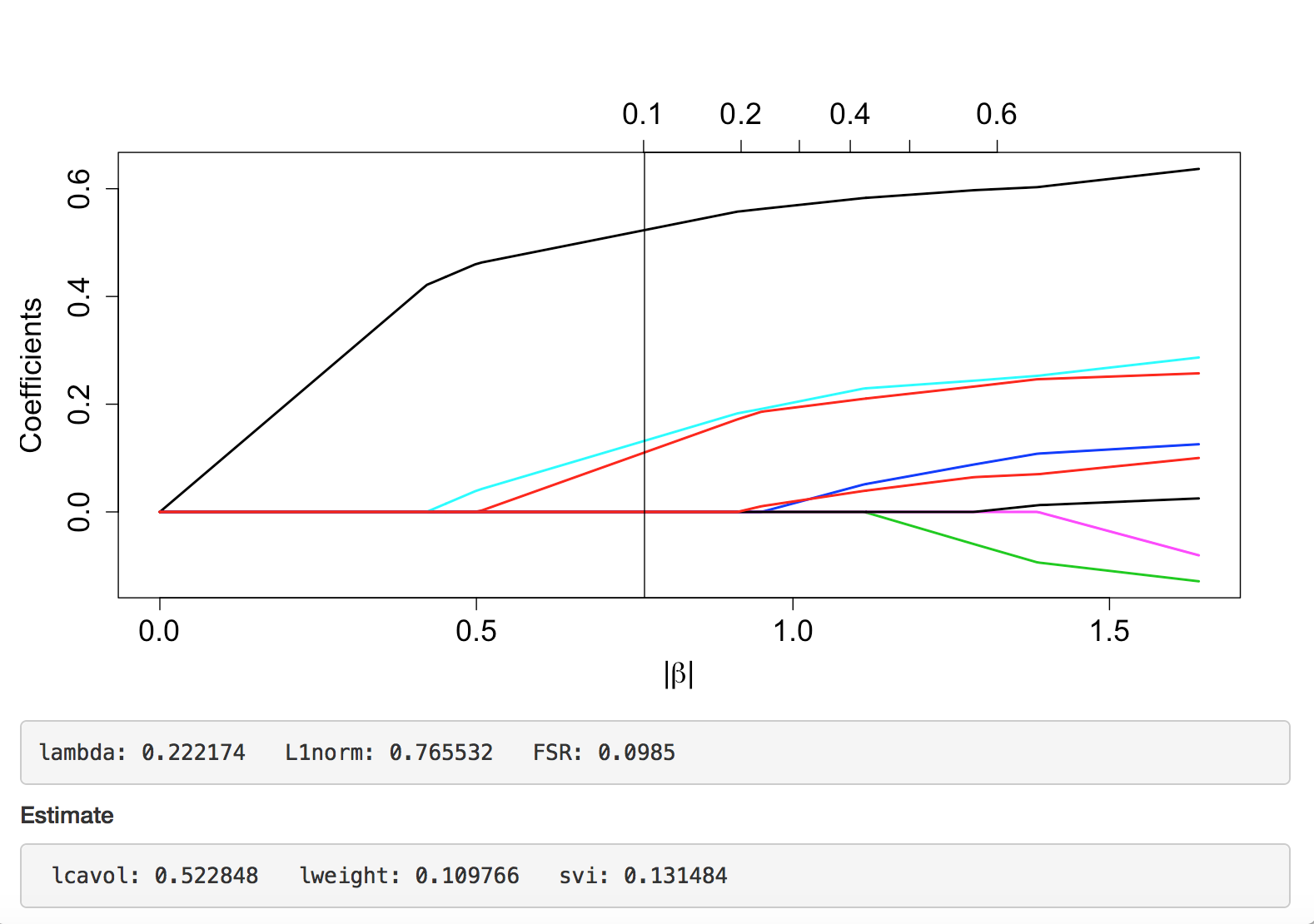
Figure 1: Lasso solution path for prostate cancer data. FSR and coefficient estimates are designed to be shown interactively.

The proposed estimator of the false selection rate depends on the generation of pseudo-variables that are conditionally independent of the response given the important variables in the model. As the true important variables are unknown in practice, our estimator consists of three steps: (i) initial variable screening to estimate the set of important variables; (ii) generation of pseudo-variables so that the covariance structure between the pseudo-variables and those selected in the screening step mimics the covariance structure between the not-selected and selected variables in the screening step; and (iii) fitting the penalized estimator and using the proportion of selected pseudo-variables to construct an estimator of the false selection rate. The proposed methodology is an example of a noise-variable or knock-off variable method. Such methods have been applied to control the false selection rate in forward selection (Wu et al., 2007) and for the Lasso (Barber and Candès, 2015; Barber and Candès, 2016). A primary contribution of this work is an estimator of the false selection rates for a sequence of tuning parameter values $\lambda_{(1)},\lambda_{(2)},\ldots,\lambda_{(m)}$ along the solution path that applies when $p\gg n$. When the proposed method is used to tune the amount of penalization so as to achieve a target false selection rate, it provides better empirical performance than alternatives in simulation experiments. Our theoretical and methodological developments focus on a linear model estimated using the Lasso (Tibshirani, 1996) under a fixed design; however, simulation experiments illustrate broader applicability. To facilitate the interactive model building, we have implemented the proposed methods in an R package and a shiny web application both of which are contained in the Supplemental Materials.

In Section 2, we establish notation, describe the proposed estimator, and state some of its theoretical properties. In Section 3, we demonstrate the finite-sample performance of the proposed method in a suite of simulation experiments. In Section 4, we illustrate application of the proposed method using the data from prostate cancer study and leukemia cancer study. Concluding remarks are made in Section 5.

2 Methods

2.1 Setup and notation

We consider data from a linear model under a fixed design. The observed data are $\left\{(X_{i},Y_{i})\right\}_{i=1}^{n}$ and it is assumed that $Y_{i}=X_{i}^{\intercal}\beta_{0}+\epsilon_{i}$, where $\epsilon_{1},\ldots,\epsilon_{n}\buildrel iid\over{\sim}\mathrm{Normal}(0,\sigma^{2})$, and $\beta_{0}=(\beta_{0,1},\ldots,\beta_{0,p})^{\intercal}\in\mathbb{R}^{p}$. Define $\mathbb{X}=(X_{1},\ldots,X_{n})^{\intercal}\in\mathbb{R}^{n\times p}$ and $\mathbb{Y}=(Y_{1},\ldots,Y_{n})^{\intercal}$. Given tuning parameter $\lambda>0$, the Lasso estimator of $\beta_{0}$ is

$$\widehat{\beta}_{n}(\lambda;\mathbb{Y},\mathbb{X})=\arg\min_{\beta\in\mathbb{R}^{p}}\left\{\frac{1}{2n}||\mathbb{Y}-\mathbb{X}\beta||^{2}+\lambda\sum_{j=1}^{p}|\beta_{j}|\right\}.$$

Define $A_{0}=\left\{j\,:\,\beta_{0,j}\neq 0\right\}$ to be the index set of nonzero coefficients in the true model and let $\widehat{A}_{n}(\lambda)=\left\{j\,:\,\widehat{\beta}_{n,j}(\lambda;\mathbb{Y},\mathbb{X})\neq 0\right\}$ denote the active set at $\lambda$. For any $S\subseteq\left\{1,\ldots,p\right\}$, write $\mathbb{X}_{S}$ to denote the design matrix composed of variables indexed by $S$; let $S^{c}$ denote the complement of $S$ and $\mathcal{N}(S)$ the number of elements in $S$. Define $\boldsymbol{\Sigma}=n^{-1}\left(\mathbb{X}_{A_{0}},\mathbb{X}_{A_{0}^{C}}\right)^{T}\left(\mathbb{X}_{A_{0}},\mathbb{X}_{A_{0}^{C}}\right)$; $\widehat{I}_{n}(\lambda)=\mathcal{N}\left\{\widehat{A}_{n}(\lambda)\bigcap A_{0}\right\}$; and $\widehat{U}_{n}(\lambda)=\mathcal{N}\left\{\widehat{A}_{n}(\lambda)\setminus A_{0}\right\}$. Thus, the false selection rate at $\lambda$ is $p_{n}(\lambda)=E\left[\widehat{U}_{n}(\lambda)/\max\left\{\widehat{I}_{n}(\lambda)+\widehat{U}_{n}(\lambda),1\right\}\right]$.

2.2 Estimating the false selection rate

In this section, we provide a description of our estimator of the false selection rate for each model along the Lasso solution path and provide theoretical justification; details of the implementation are deferred to the subsequent section. The proposed estimator is constructed in three stages: (S1) apply screening to form a preliminary estimator of the set of nonzero coefficients, $A_{0}$; (S2) generate pseudo-variables that mimic the unimportant variables, i.e., those in $A_{0}^{c}$; and (S3) apply the Lasso to a dataset composed of the selected variables from the screening step and the generated pseudo-variables; the proportion of pseudo-variables in the active set, $\widehat{A}_{n}(\lambda)$, is the estimated false selection rate at tuning parameter value $\lambda$.

Let $r=rank(\mathbf{\mathbb{X}})$ and for any square matrix, $U$, write $U^{-}$ to denote a pseudo-inverse. For any non-empty subset $S$ of $\left\{1,\ldots,p\right\}$, define $Q_{11}(S)=n^{-1}\mathbb{X}_{S}^{\intercal}\mathbb{X}_{S}$, $Q_{12}(S)=n^{-1}\mathbb{X}_{S}^{\intercal}\mathbb{X}_{S^{c}}$, $Q_{21}(S)=n^{-1}\mathbb{X}_{S^{c}}^{\intercal}\mathbb{X}_{S}$, $Q_{22}(S)=n^{-1}\mathbb{X}_{S^{c}}^{\intercal}\mathbb{X}_{S^{c}}$, and $P_{\mathbb{X}_{S}}=\mathbb{X}_{S}(\mathbb{X}_{S}^{\intercal}\mathbb{X}_{S})^{-}\mathbb{X}_{S}^{\intercal}$. The estimator $\widehat{p}_{n}(\lambda)$ of $p_{n}(\lambda)$ is constructed as follows.

• Step 1 (Screening): For the full data $(\mathbb{X},\mathbb{Y})$, apply a viable variable selection method to construct a preliminary estimator, $\widehat{A}_{0,n}$, of the set of nonzero coefficients $A_{0}$. Let $\widehat{r}_{0}$ denote the rank of $\mathbb{X}_{\widehat{A}_{0,n}}$.

• Step 2 (Pseudo-variable generation): Let $\Omega(\widehat{A}_{0,n})\in\mathbb{R}^{(r-\widehat{r}_{0})\times\left\{p-\mathcal{N}(\widehat{A}_{0,n})\right\}}$ satisfy

  $$\Omega(\widehat{A}_{0,n})^{\intercal}\Omega(\widehat{A}_{0,n})=Q_{22}(\widehat{A}_{0,n})-Q_{21}(\widehat{A}_{0,n})Q_{11}^{-}(\widehat{A}_{0,n})Q_{12}(\widehat{A}_{0,n}),$$

  and let $V(\widehat{A}_{0,n})\in\mathbb{R}^{n\times(r-\widehat{r}_{0})}$ be any orthonormal matrix that is orthogonal to the column space of $\mathbb{X}_{\widehat{A}_{0,n}}$. Pseudo-variables have the form

  $$\mathbb{X}_{\mathrm{pseudo}}=P_{\mathbb{X}_{\widehat{A}_{0,n}}}\mathbb{X}_{\widehat{A}_{0,n}^{c}}+\sqrt{n}V(\widehat{A}_{0,n})\Omega(\widehat{A}_{0,n}).$$ (1)

  In Section 2.3, we describe how to calculate $\Omega(\widehat{A}_{0,n})$ and generate $V(\widehat{A}_{0,n})$ randomly thereby allowing for generating replicate random pseudo-variables.

• Step 3 (Error rate estimation): Fit the Lasso estimator using $\mathbb{X}_{\mathrm{new}}=(\mathbb{X}_{\widehat{A}_{0,n}},\mathbb{X}_{\mathrm{pseudo}})$, and calculate $\widehat{A}_{n}^{\mathrm{new}}(\lambda)=\{j:\widehat{\beta}_{n,j}(\lambda;\mathbb{Y},\mathbb{X}_{\mathrm{new}})\neq 0\}$, and subsequently

  $$\widehat{p}_{n}(\lambda)=\frac{\widehat{U}_{n}^{\mathrm{new}}(\lambda)}{\max\left\{\widehat{I}_{n}^{\mathrm{new}}(\lambda)+\widehat{U}_{n}^{\mathrm{new}}(\lambda),1\right\}}=\frac{\mathcal{N}\left\{\widehat{A}_{n}^{\mathrm{new}}(\lambda)\setminus\widehat{A}_{0,n}\right\}}{\max\left[\mathcal{N}\left\{\widehat{A}_{0,n}^{\mathrm{new}}(\lambda)\right\},1\right]},$$ (2)

  where $\widehat{I}_{n}^{\mathrm{new}}(\lambda)=\mathcal{N}\left\{\widehat{A}_{n}^{\mathrm{new}}(\lambda)\bigcap\widehat{A}_{0,n}\right\}$ and $\widehat{U}_{n}^{\mathrm{new}}(\lambda)=\mathcal{N}\left\{\widehat{A}_{n}^{\mathrm{new}}(\lambda)\setminus\widehat{A}_{0,n}\right\}$.

To stabilize our estimator, we repeat the above steps $B$ times to obtain the estimators $\widehat{p}_{n}^{(1)}(\lambda),\ldots,\widehat{p}_{n}^{(B)}(\lambda)$ and subsequently compute $\overline{\widehat{p}}_{n}(\lambda)=B^{-1}\sum_{b=1}^{B}\widehat{p}_{n}^{(b)}(\lambda)$. The following results are proved in the Appendix; throughout we implicitly assume that all requisite moments exist and are finite.

Lemma 2.1.

Suppose $\widehat{A}_{0,n}=A_{0}$ with probability one, then $n^{-1}(\mathbb{X}_{\widehat{A}_{0,n}},\mathbb{X}_{\mathrm{pseudo}})^{\intercal}(\mathbb{X}_{\widehat{A}_{0,n}},\mathbb{X}_{\mathrm{pseudo}})=\boldsymbol{\Sigma}.$ Furthermore, $\left\{\widehat{I}_{n}(\lambda),\widehat{U}_{n}(\lambda)\right\}$ and $\left\{\widehat{I}_{n}^{\mathrm{new}}(\lambda),\widehat{U}_{n}^{\mathrm{new}}(\lambda)\right\}$ are equal in distribution.

The preceding result shows that were the set of important variables, $A_{0}$, known, substituting the pseudo-variables for the unimportant variables, $A_{0}^{c}$, does not affect the false selection rate. Of course, $A_{0}$ is not known in practice; the following result shows that preceding result holds provided that the initial screening procedure is selection consistent.

Theorem 2.2.

Assume that $\widehat{A}_{0,n}\rightarrow A_{0}$ with probability one. Then, for any bounded function $g:\mathbb{R}^{2}\rightarrow\mathbb{R}$, it follows that

$$\sup_{\lambda}\left|E\left[g\left\{\widehat{I}_{n}(\lambda),\widehat{U}_{n}(\lambda)\right\}\right]-E\left[g\left\{\widehat{I}_{n}^{\mathrm{new}}(\lambda),\widehat{U}_{n}^{\mathrm{new}}(\lambda)\right\}\right]\right|=o(1).$$

Corollary 2.3.

Assume that $\widehat{A}_{0,n}\rightarrow A_{0}$ with probability one. Then, for any bounded function $g:\mathbb{R}^{2}\rightarrow\mathbb{R}$, it follows that

$$\sup_{\lambda,t}\left|P\left[g\left\{\widehat{I}_{n}(\lambda),\widehat{U}_{n}(\lambda)\right\}\leq t\right]-P\left[g\left\{\widehat{I}_{n}^{\mathrm{new}}(\lambda),\widehat{U}_{n}^{\mathrm{new}}(\lambda)\right\}\leq t\right]\right|=o(1).$$

Corollary 2.4.

Assume $\widehat{A}_{0,n}\rightarrow A_{0}$ with probability one. Then, setting $g(v,w)=v/\max(v+w,1)$ shows

$$\sup_{\lambda}\left|p_{n}(\lambda)-B^{-1}\sum_{b=1}^{B}E\left\{\widehat{p}^{b}_{n}(\lambda)\right\}\right|=o(1).$$

The preceding results require a selection-consistent screening procedure; we provide such a selection procedure based on pseudo-variables in the Supplemental Materials. While the theoretical assumption of selection consistency might be still strong, empirical results in the next section suggest that screening based on Lasso tuned by 10-fold cross validation (which is not selection consistent) leads to satisfactory results.

In small samples, we have found that the empirical performance of our procedure can be improved by augmenting $\mathbb{X}_{\mathrm{new}}$ with a permutation of $\mathbb{X}_{\widehat{A}_{0,n}}$, say $\mathbb{X}_{\mathrm{perm}}=(\mathbb{X}_{\widehat{A}_{0,n}},\mathbb{X}_{\mathrm{pseudo}},G\mathbb{X}_{\widehat{A}_{0,n}})$ where $G$ is a random permutation matrix. The intuition for adding this permutation is to compensate for over-estimation of $A_{0}$ in finite samples (which in turn leads to underestimation of the false selection rate). See Proposition 1.1 in the Supplemental Materials for an analog of Corollary 2.4 for this modified procedure.

Control of the FSR at specified error rate $\alpha$ is achieved by first estimating the FSRs for a sequence of tuning parameter values, $\lambda_{(1)},\ldots,\lambda_{(m)}$ and then selecting the tuning parameter $\widehat{\lambda}=\min\{\lambda_{(i)}:\widehat{p}(\lambda_{(i)})\leq\alpha\}$. The final model is obtained by fitting the Lasso using $(\mathbb{X},\mathbb{Y})$ at tuning parameter $\widehat{\lambda}$.

2.3 Computation of pseudo-variables

Our procedure for generating pseudo-variables is based on the following result which is proved in the Supplemental Materials.

Lemma 2.5.

For any non-empty subset $S$ of $\left\{1,\ldots,p\right\}$ such that $\mathbb{X}_{S}$ has rank $r(S)$, denote $s=\mathcal{N}(S)$. Then $\left\{\mathbb{X}_{S},\mathbb{X}_{\mathrm{pseudo}}(S)\right\}^{\intercal}\left\{\mathbb{X}_{S},\mathbb{X}_{\mathrm{pseudo}}(S)\right\}=\left(\mathbb{X}_{S},\mathbb{X}_{S^{c}}\right)^{\intercal}\left(\mathbb{X}_{S},\mathbb{X}_{S^{c}}\right)$ if and only if $\mathbb{X}_{\mathrm{pseudo}}(S)=P_{\mathbb{X}_{S}}\mathbb{X}_{S^{c}}+\sqrt{n}V(S)\Omega(\mathbb{X},S)$ for some $V(S)$ and $\Omega(\mathbb{X},S)$, where $V(S)$ is an $n\times\left\{r-r(S)\right\}$ orthonormal matrix that is orthogonal to $\mathbb{X}_{S}$, and $\Omega(\mathbb{X},S)$ is an $\left\{r-r(S)\right\}\times\left\{p-s\right\}$ matrix such that $\Omega(\mathbb{X},S)^{\intercal}\Omega(\mathbb{X},S)=Q_{22}(S)-Q_{21}(S)Q_{11}^{-}(S)Q_{12}(S)$.

Thus, the preceding result characterizes a class of potential pseudo-variables indexed by the matrices $V(S)$ and $\Omega(\mathbb{X},S)$.

To generate pseudo-variables, the first part $P_{\mathbb{X}_{S}}\mathbb{X}_{S^{c}}$ is calculated directly using a QR decomposition. The second part, $V(S)$, is constructed using the form $V(S)=V_{1}V_{2},$ where $V_{1}$ is an $n\times\left\{n-r(S)\right\}$ orthonormal matrix which is orthogonal to $\mathbb{X}_{S}$, and $V_{2}$ is a random orthonormal matrix. To find $V_{1}$, we compute the QR decomposition $\mathbb{X}_{S}=Q_{x}R_{x}$ and then choose $V_{1}$ to be the last $n-r(S)$ columns of $Q_{x}$, which are an orthonormal basis for the null space of $\mathbb{X}_{S}^{T}$. Subsequently, $V_{2}$ is a random orthonormal matrix distributed with Haar measure Mezzadri (2006).

To find $\Omega$ such that $\Omega(\mathbb{X},S)^{\intercal}\Omega(\mathbb{X},S)=Q_{22}(S)-Q_{21}(S)Q_{11}^{-}(S)Q_{12}(S)$, it is not necessary to compute $Q_{22},Q_{21},Q_{11}$, which is computationally expensive for $p\gg n$. To see this, define $\mathcal{E}_{1|2}=(I-P_{\mathbb{X}_{S}})\mathbb{X}_{S^{c}}$ so that $\mathcal{E}_{1|2}^{\intercal}\mathcal{E}_{1|2}=(Q_{22}-Q_{21}Q_{11}^{-}Q_{12})$, then compute the QR decomposition $\mathcal{E}_{1|2}=Q_{\mathcal{E}}R_{\mathcal{E}}$ and choose $\Omega$ to be the first $r-r(S)$ rows of $R_{\mathcal{E}}$.

3 Simulations

We examine the finite-sample performance of the proposed method in terms of FSR control and true selection rate (TSR) across data sets with varying dimension, number of nonzero coefficients, signal strength, and correlation structure. Our examination is based on the comparison of the following methods: pseudo-1, the proposed variable addition method with the screening procedure given in the Supplemental Materials; pseudo-2, the proposed variable addition method with the screening done using the Lasso tuned with 10-fold cross-validation; Knockoff and Knockoff+ (Barber and Candès, 2015); and pseudo-Wu, a variable-addition method proposed to control FSR in forward selection (Wu et al., 2007).

In implementing our proposed methods we included the permutation term as discussed in Section 2; results without the permutation are presented in the Supplemental Materials. In our implementation of the proposed pseudo-variable methods, we repeated pseudo-variable generation $B=20$ times in each iteration. The knockoff and knockoff+ methods, are as implemented in the R package knockoff with default parameter settings. The pseudo-Wu is as implemented on the authors’ website. Their implementation requires $n>2p$ so that $p$-values for all variables can be calculated. As suggested by the authors, we use a bootstrap size $B=200$ for the pseudo-Wu method.

The data are generated from the linear model $Y_{i}=X_{i}^{T}\boldsymbol{\beta}_{0}+\epsilon_{i},\ i=1,\ldots n,$ where $\epsilon_{i}\sim N(0,1)$ and $X_{i}\sim~{}N(0_{p\times 1},C)$ with $C_{ij}=\rho^{|i-j|}$. Define $\boldsymbol{\beta}_{0}=(A,A,0,0,A,0,\ldots,0,0)^{t}$, where $A$ is the signal amplitude and positions of nonzero coefficient are sampled without replacement from $\{1,\ldots,p\}$. Denote the number of nonzero coefficients by $s$.

We study four different factors thought to influence FSR/TSR estimation:

• predictor dimension: we fix $n=200,\ \rho=0.5,\ A=1,\ s=5$, and vary $p=30$, $70$, $110$, $150,\ 190,\ 230,\ 330,\ 430,\ 530$;

• correlation magnitudes: we fix $n=200,\ p=50,\ A=1,\ s=5$, and vary $\rho=0,\ 0.1$, $0.2$, $\ldots,0.8,\ 0.9$;

• signal amplitude: we fix $n=200,\ p=50,\ \rho=0.5,\ s=5$, and vary $A=0.1,\ 0.2,\ 0.3,\ \ldots,\ 1$;

• number of nonzero coefficients: we fix $n=200,\ p=50,\ \rho=0.5,\ A=1$, and vary $s=1,\ 2,\ 3,\ \ldots,\ 20$.

For each of the above combinations of parameter values, we first generate twenty different values of $\boldsymbol{\beta}_{0}$ and then for each $\boldsymbol{\beta}_{0}$, we generate $50$ datasets. Thus, for each combination of parameter values, we generate 1,000 replicates. Results are based on the average across these replicates. In all settings, we set $\alpha=0.20$, to be the target false selection rate; results for additional values of $\alpha$ are given in the Supplemental Materials.

Simulation performance across the different parameter settings are displayed in Figures 2-4. Standard errors of the FSR and TSR averages are less than 0.015 for all simulation settings. It can be seen that the proposed methods are consistently less biased than alternatives in terms of FSR. For TSR, knockoff and knockoff+ decrease rapidly as $p\rightarrow n$. Furthermore, when number of true signal is sparse, i.e., when $s$ is small, knockoff+ and Pseudo-Wu have low power.

Both of the proposed pseudo-variable methods performed favorably relative to competing methods. That pseudo-2 performed well is encouraging as it does not satisfy the selection consistency criterion required in our theoretical results, suggesting that the proposed pseudo-variable methods are robust to mild violations of this assumption. Furthermore, in the Supplemental Materials, we present application of the proposed methods to a Cox proportional hazards model as well as a logistic regression model; these simulations are qualitatively similar to those presented here suggesting the proposed method can be applied more generally than the linear model case for which our theory was developed.

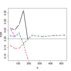
(a) False selection rate vs $p$

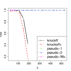
(b) True selection rate vs $p$

Figure 2: Performances under different dimensions at $\alpha=0.2$. Left and right figure shows the average FSR and TSR respectively. The Knockff and Knockoff methods require $n>p$ and the Wu’s pseudo-variable method requires $n>2p$.

(a) False selection rate vs $\rho$

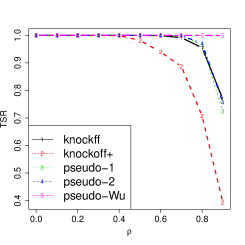
(b) True selection rate vs $\rho$

Figure 3: Performances under different correlations at $\alpha=0.2$. Left and right figure shows the average FSR and TSR respectively.

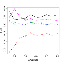
(a) False selection rate vs $A$

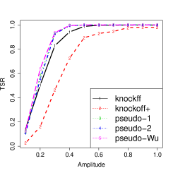
(b) True selection rate vs $A$

Figure 4: Performances under different coefficient amplitude at $\alpha=0.2$. Left and right figure shows the average FSR and TSR respectively.

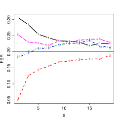
(a) False selection rate vs $s$

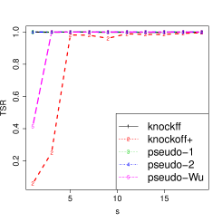
(b) True selection rate vs $s$

Figure 5: Performances under different number of nonzero coefficients at $\alpha=0.2$. Left and right figure shows the average FSR and TSR respectively.

4 Illustrative examples

4.1 Prostate cancer data

Our first illustrative example uses data from a study of prostate specific antigen (PSA) in $n=97$ prostate cancer patients (Stamey et al., 1989). One of the goals of the study was to understand the relationship between PSA and eight biomarkers: log cancer volume (lcavol); log prostate weight (lweight); age in years (age); log of the amount of benign prostatic hyperplasia (lbph); seminal vesicle invasion (svi); log of capsular penetration (lcp); Gleason score (gleason); and percent of Gleason scores 4 or 5 (pgg45).

As in previous analyses, we fit a linear model for the regression of log PSA (lpsa) on the preceding eight biomarkers. We fit the model using the proposed pseudo-variable method with screening done using the Lasso tuned using 10-fold cross validation, and $B=100$ resamples. The Lasso solution path is presented in Figure 6. The vertical line on the left corresponds to an estimated FSR of $\widehat{\alpha}=0.1$; the associated model has three predictors: lcavol, lweight, svi. The middle vertical line corresponds to an estimated FSR of $\widehat{\alpha}=0.2$; the associated model has four predictors: lcavol, lweight, svi, pgg45. The right vertical line corresponds to an estimated FSR of $\widehat{\alpha}=0.3$; the associated model has five predictors: lcavol, lweight, svi, pgg45, lbph.

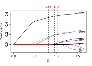
Figure 6: Lasso solution path for prostate cancer data. Vertical lines from left to right correspond to estimated FSRs of $\alpha=0.1$, $\alpha=0.2$, and $\alpha=0.3$.

4.2 Leukemia cancer gene expression data

Our second illustrative example used data from leukemia study (see Efron, 2012). The primary outcome is binary cancer type: acute myeloid leukemia (AML) or acute lymphoblastic leukemia (ALL). The goal is understand how gene expression data relates to cancer type. Expression levels are measured for $p=7128$ genes on $n=72$ subjects. Thus, this second example demonstrates the use of the proposed method in the $p\gg n$ setting.

We fit a penalized logistic regression model for cancer type on gene expression levels. To estimate FSR, screening is done using the Lasso tuned using 10-fold cross validation, and we set $B=100$. The Lasso solution path with estimated FSRs is displayed in Figure 6. The vertical lines on the figure, read from left to right, correspond to estimated FSRs of $\widehat{\alpha}=0.1,0.2$ and $0.3$; it can be seen that these correspond to four, six and eleven selected genes. The choice of an appropriate model along this path should be dictated by the costs associated with a false positive and other domain-specific considerations.

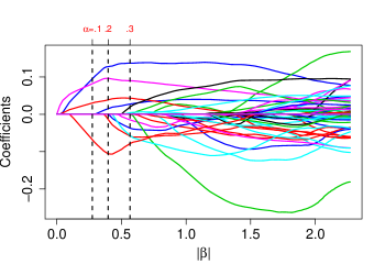
Figure 7: Lasso solution path for leukemia cancer gene expression data. Vertical lines from left to right correspond to estimated FSRs of $\alpha=0.1$, $\alpha=0.2$, and $\alpha=0.3$.

5 Conclusion

We proposed a novel variable-addition method to estimate the FSR in penalized regression. The proposed method provides (asymptotically) unbiased estimates of the FSR uniformly over the solution path even when $p\gg n$. The primary motivation for the proposed methodology was to label the solution path with estimated operating characteristics that are meaningful in a domain context. While our focus was on linear models with a fixed design, simulation results suggest broader applicability. Indeed, one of the appealing features of variable-addition methods is that they can be applied (at least in principle) to black-box models. Evaluation of the theoretical properties of the proposed method to such models is a topic for future research.

SUPPLEMENTARY MATERIAL

Simulation results:

Additional simulation results are presented in the online supplement to this article.

Phony-variables algorithm for screening:

Details of pseudo-variables algorithm for screening with proof of selection consistency.

Proofs and technical details:

Detailed proofs are provided in the online supplement to this article.

R package:

A R package is provided in the online supplement to this article.

6 Proof and Technical Details

See 2.1

Proof.

First for $n^{-1}(\mathbb{X}_{\widehat{A}_{0}})^{\intercal}\mathbb{X}_{\mathrm{pseudo}}$, we have

$$n^{-1}(\mathbb{X}_{\widehat{A}_{0}})^{\intercal}\mathbb{X}_{\mathrm{pseudo}}$$

$$=n^{-1}(\mathbb{X}_{\widehat{A}_{0}})^{\intercal}\left\{P_{\mathbb{X}_{\widehat{A}_{0}}}\mathbb{X}_{\widehat{A}_{0}^{c}}+\sqrt{n}V\Omega\right\}$$

$$=Q_{12}(A_{0}),$$

where the last equality holds since $V$ is orthogonal to the column space of $\mathbb{X}_{\widehat{A}_{0}}$.

Then,

$$n^{-1}\mathbb{X}_{\mathrm{pseudo}}^{\intercal}\mathbb{X}_{\mathrm{pseudo}}$$

$$=n^{-1}\left\{P_{\mathbb{X}_{\widehat{A}_{0}}}\mathbb{X}_{\widehat{A}_{0}^{c}}+\sqrt{n}V\Omega\right\}^{\intercal}\left\{P_{\mathbb{X}_{\widehat{A}_{0}}}\mathbb{X}_{\widehat{A}_{0}^{c}}+\sqrt{n}V\Omega\right\}$$

$$=\left\{n^{-1}\mathbb{X}_{\widehat{A}_{0}^{c}}^{\intercal}P_{\mathbb{X}_{\widehat{A}_{0}}}P_{\mathbb{X}_{\widehat{A}_{0}}}\mathbb{X}_{\widehat{A}_{0}^{c}}\right\}+\left\{\Omega^{\intercal}\Omega\right\}$$

$$=\left\{n^{-1}\mathbb{X}_{\widehat{A}_{0}^{c}}^{\intercal}\left[\mathbb{X}_{\widehat{A}_{0}}\{\mathbb{X}_{\widehat{A}_{0}}^{\intercal}\mathbb{X}_{\widehat{A}_{0}}\}^{-}\mathbb{X}_{\widehat{A}_{0}}^{\intercal}\right]\mathbb{X}_{\widehat{A}_{0}^{c}}\right\}+\left\{\Omega^{\intercal}\Omega\right\}$$

$$=Q_{21}Q_{11}^{-}Q_{12}+(Q_{22}-Q_{21}Q_{11}^{-}Q_{12})$$

$$=Q_{22}(\widehat{A}_{0}).$$

This completes the proof that

$$n^{-1}(\mathbb{X}_{\widehat{A}_{0}},\mathbb{X}_{\mathrm{pseudo}})^{\intercal}(\mathbb{X}_{\widehat{A}_{0}},\mathbb{X}_{\mathrm{pseudo}})=\boldsymbol{\Sigma}.$$

Then we know, $n^{-1/2}(\mathbb{X}_{\widehat{A}_{0}},\mathbb{X}_{\mathrm{pseudo}})^{T}\boldsymbol{\epsilon}$ follows a multivariate normal distribution with mean $\mathbf{0}$ and covariance $\boldsymbol{\Sigma}$, which is the same as distribution of $n^{-1/2}(\mathbb{X}_{A_{0}},\mathbb{X}_{{\widehat{A}_{0}}^{c}})\boldsymbol{\epsilon}$. Since the Lasso solution only depends on $\boldsymbol{\Sigma}$ and $(\mathbb{X}_{\widehat{A}_{0}},\mathbb{X}_{\mathrm{pseudo}}^{T}\boldsymbol{\epsilon})$, we have that $\left(\widehat{I}_{n}\left(\lambda\right),\widehat{U}_{n}(\lambda)\right)$ and $\left(\widehat{I}_{n}^{\mathrm{new}}\left(\lambda\right),\widehat{U}_{n}^{\mathrm{new}}(\lambda)\right)$ are identically distributed. ∎

See 2.2

Proof.

First, we have

$$\sup_{\lambda}\left|E\left\{g\left(\widehat{I}_{n}^{\mathrm{new}}(\lambda),\widehat{U}_{n}^{\mathrm{new}}(\lambda)\right)\mid\widehat{A}_{0,n}=A_{0}\right\}-E\left\{g\left(\widehat{I}_{n}^{\mathrm{new}}(\lambda),\widehat{U}_{n}^{\mathrm{new}}(\lambda)\right)\right\}\right|=o(1).$$ (3)

This follows from

$$E\left\{g\left(\widehat{I}_{n}^{\mathrm{new}}(\lambda),\widehat{U}_{n}^{\mathrm{new}}(\lambda)\right)\right\}$$

$$=E\left\{g\left(\widehat{I}_{n}^{\mathrm{new}}(\lambda),\widehat{U}_{n}^{\mathrm{new}}(\lambda)\right)\mid\widehat{A}_{0,n}=A_{0}\right\}P(\widehat{A}_{0,n}=A_{0})$$

$$+E\left\{g\left(\widehat{I}_{n}^{\mathrm{new}}(\lambda),\widehat{U}_{n}^{\mathrm{new}}(\lambda)\right)\mid\widehat{A}_{0,n}\neq A_{0}\right\}P(\widehat{A}_{0,n}\neq A_{0}),$$

and $P(\widehat{A}_{0,n}=A_{0})=1-o(1)$.

Then, suppose modifying screening step to be deterministic, one constructs pseudo-variables always using the true active set, i.e., $\mathbb{X}_{\mathrm{pseudo}}=P_{\mathbb{X}_{A_{0}}}\mathbb{X}_{A_{0}^{c}}+\sqrt{n}V(A_{0})\Omega(A_{0})$. Denote the corresponding number of important variables at $\lambda$ as $\widehat{I}_{n}^{1}(\lambda)$, the number of unimportant variables at $\lambda$ as $\widehat{U}_{n}^{1}(\lambda)$. Then we have

$$\sup_{\lambda}\left|E\left\{g\left(\widehat{I}_{n}^{\mathrm{new}}(\lambda),\widehat{U}_{n}^{\mathrm{new}}(\lambda)\right)\mid\widehat{A}_{0,n}=A_{0}\right\}-E\left\{g\left(\widehat{I}_{n}^{1}(\lambda),\widehat{U}_{n}^{1}(\lambda)\right)\right\}\right|=o(1).$$ (4)

And by Lemma 2.1

$$\sup_{\lambda}\left|E\left\{g\left(\widehat{I}_{n}(\lambda),\widehat{U}_{n}(\lambda)\right)\right\}-E\left\{g\left(\widehat{I}_{n}^{1}(\lambda),\widehat{U}_{n}^{1}(\lambda)\right)\right\}\right|=o(1).$$ (5)

Therefore, the results follow by combining eq. (3), (4) and (5). ∎

See 2.3 See 2.4

Proof.

Corollary 2.3 and Corollary 2.4 are immediate results from Theorem 2.2. ∎

See 2.5

Proof.

Sufficient condition is proven by similar argument of Lemma 2.1. It is remaining to prove necessary condition. First, we should have $\mathbb{X}_{S}^{\intercal}\mathbb{X}_{\mathrm{pseudo}}=\mathbb{X}_{S}^{\intercal}\mathbb{X}_{S^{c}}$. Therefore, $\mathbb{X}_{\mathrm{pseudo}}$ should have the form $\mathbb{X}_{\mathrm{pseudo}}=\mathbb{X}_{S^{c}}+V_{\epsilon}$, where $V$ is a matrix orthogonal to column space of $\mathbb{X}_{S}$. Then

$$\mathbb{X}_{\mathrm{pseudo}} =\mathbb{X}_{S^{c}}+V_{\epsilon}$$

$$=\mathbb{X}_{S^{c}}+(I-P_{\mathbb{X}_{S}})\mathbb{X}_{S^{c}}+V_{\epsilon}-(I-P_{\mathbb{X}_{S}})\mathbb{X}_{S^{c}}$$

$$=P_{\mathbb{X}_{S}}\mathbb{X}_{S^{c}}+V^{*}_{\epsilon},$$

where $V^{*}_{\epsilon}$ is a matrix orthogonal to column space of $\mathbb{X}_{S}$. Express $V^{*}_{\epsilon}$ to be $V^{*}_{\epsilon}=\sqrt{n}VA$, where $V$ is an orthonormal matrix that orthogonal to column space of $\mathbb{X}_{S}$ and $A$ to be any matrix with right dimension.

Then we will prove $A^{T}A=(Q_{22}-Q_{21}Q_{11}^{-}Q_{12})$. To satisfy condition that $\mathbb{X}_{\mathrm{pseudo}}^{\intercal}\mathbb{X}_{\mathrm{pseudo}}=\mathbb{X}_{S^{c}}^{\intercal}\mathbb{X}_{S^{c}}$. Namely, $\left(P_{\mathbb{X}_{S}}\mathbb{X}_{S^{c}}+\sqrt{n}VA\right)^{\intercal}\left(P_{\mathbb{X}_{S}}\mathbb{X}_{S^{c}}+\sqrt{n}VA\right)=\mathbb{X}_{S^{c}}^{\intercal}\mathbb{X}_{S^{c}}$. By simple calculation, we have $nA^{\intercal}A=\mathbb{X}_{S^{c}}^{\intercal}(I-P_{\mathbb{X}_{S}})\mathbb{X}_{S^{c}}$. Therefore, $A^{T}A=(Q_{22}-Q_{21}Q_{11}^{-}Q_{12})$.

∎

6.1 Proof of error rate estimation with permutation added

Suppose that fitting Lasso with $(\mathbb{X},G\mathbb{X}_{\widehat{A}_{0,n}},Y)$, denote the corresponding number of unimportant variables and important variables at $\lambda$ as $\widehat{U}^{*}_{n}(\lambda)$ and $\widehat{I}^{*}_{n}(\lambda)$ respectively. Assume $E[U^{*}_{n}(\lambda)/\max\{U^{*}_{n}(\lambda)+I^{*}_{n}(\lambda),1\}]\geq E[\widehat{U}_{n}/\max\{\widehat{U}_{n}+\widehat{I}_{n},1\}]$, then we have the following result

Proposition 6.1.

If $\lim_{n\rightarrow\infty}P(\widehat{A}_{0,n}=A_{0})=1$, then $\sup_{\lambda}\left\{E(\widehat{p}_{n}(\lambda))-p_{n}(\lambda)\right\}\geq o(1)$.

Proof.

By similar argument with the proof of Theorem 2.2, we have

$$\sup_{\lambda}\left[E\left(\widehat{p}_{n}(\lambda)\right)-E\left\{\frac{\widehat{U}^{*}_{n}(\lambda)}{\max(\widehat{U}^{*}_{n}(\lambda)+\widehat{I}^{*}_{n}(\lambda),1)}\right\}\right]=o(1).$$

Then combining with the assumption above, we have $\sup_{\lambda}\left\{E(\widehat{p}_{n}(\lambda))-p_{n}(\lambda)\right\}\geq o(1)$. ∎

Remark.

The assumption $E[U^{*}_{n}(\lambda)/\max\{U^{*}_{n}(\lambda)+I^{*}_{n}(\lambda),1\}]\geq E[\widehat{U}_{n}/\max\{\widehat{U}_{n}+\widehat{I}_{n},1\}]$ implies that FSR is higher if more unimportant variables are used to fit Lasso. One can easily verify the assumption if $G\mathbb{X}_{A_{0}}$ is orthogonal to $\mathbb{X}$.

To remove the assumption $E[U^{*}_{n}(\lambda)/\max\{U^{*}_{n}(\lambda)+I^{*}_{n}(\lambda),1\}]\geq E[\widehat{U}_{n}/\max\{\widehat{U}_{n}+\widehat{I}_{n},1\}]$, one can modify the estimator as $\widehat{p}_{n}(\lambda)=\max\{\widehat{p}_{n,1}(\lambda),\{\widehat{p}_{n,2}(\lambda)\}$, where $\widehat{p}_{n,1}(\lambda)$ and $\widehat{p}_{n,2}(\lambda)$ is the FSR estimated at $\lambda$ using the method with and without permutation added respectively. Then $\sup_{\lambda}\left\{E(\widehat{p}_{n}(\lambda))-p_{n}(\lambda)\right\}\geq o(1)$ follows from

$$\sup_{\lambda}\left[E(\widehat{p}_{n,2}(\lambda))-E\left\{\widehat{U}_{n}/\max\{\widehat{U}_{n}+\widehat{I}_{n},1\}\right\}\right]\geq o(1).$$

However, it may double the computational complexity, while no significant benefits is observed in the simulation studies since $\widehat{p}_{n,1}(\lambda)$ is usually bigger than $\widehat{p}_{n,2}(\lambda)$.

7 Simulation results for $\alpha=0.1,0.3$

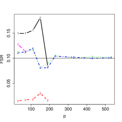
(a) False selection rate vs $p$

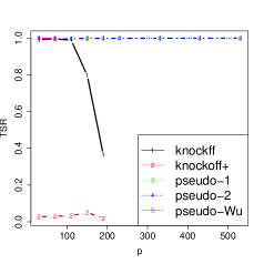
(b) True selection rate vs $p$

Figure 8: Penalized regression; Performances under different dimensions at $\alpha=0.1$.

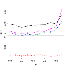
(a) False selection rate vs $\rho$

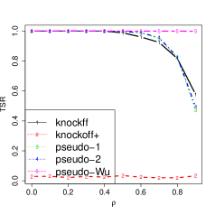
(b) True selection rate vs $\rho$

Figure 9: Penalized regression; Performances under different correlations at $\alpha=0.1$.

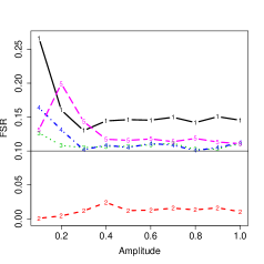
(a) False selection rate vs $A$

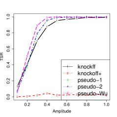
(b) True selection rate vs $A$

Figure 10: Penalized regression; Performances under different coefficient amplitude at $\alpha=0.1$.

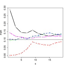
(a) False selection rate vs $s$

(b) True selection rate vs $s$

Figure 11: Penalized regression; Performances under different number of nonzero coefficients at $\alpha=0.1$.

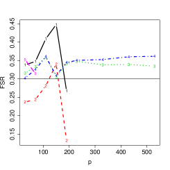
(a) False selection rate vs $p$

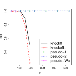
(b) True selection rate vs $p$

Figure 12: Penalized regression; Performances under different dimensions at $\alpha=0.3$.

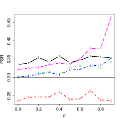
(a) False selection rate vs $\rho$

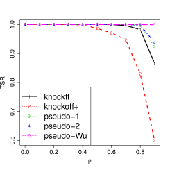
(b) True selection rate vs $\rho$

Figure 13: Penalized regression; Performances under different correlations at $\alpha=0.3$.

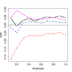
(a) False selection rate vs $A$

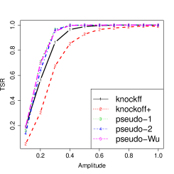
(b) True selection rate vs $A$

Figure 14: Penalized regression; Performances under different coefficient amplitude at $\alpha=0.3$.

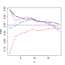
(a) False selection rate vs $s$

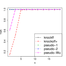
(b) True selection rate vs $s$

Figure 15: Penalized regression; Performances under different number of nonzero coefficients at $\alpha=0.3$.

8 Simulation results without adding permutation

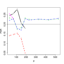
(a) False selection rate vs $p$

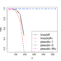
(b) True selection rate vs $p$

Figure 16: Results without permutation added; Performances under different dimensions at $\alpha=0.2$

(a) False selection rate vs $\rho$

(b) True selection rate vs $\rho$

Figure 17: Results without permutation added; Performances under different correlations at $\alpha=0.2$

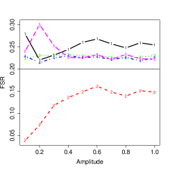
(a) False selection rate vs $A$

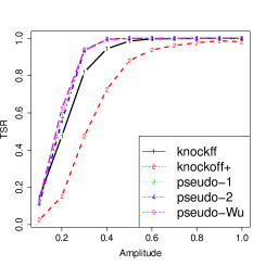
(b) True selection rate vs $A$

Figure 18: Results without permutation added; Performances under different coefficient amplitude at $\alpha=0.2$

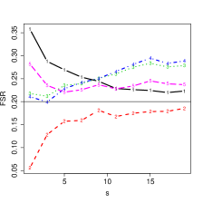
(a) False selection rate vs $s$

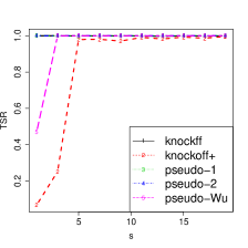
(b) True selection rate vs $s$

Figure 19: Results without permutation added; Performances under different number of nonzero coefficients at $\alpha=0.2$

9 Simulation results for logistic model

In this section, we apply the pseudo-variable method to the penalized logistic model. The Lasso estimator for logistic model at $\lambda$ is defined as

$$\widehat{\boldsymbol{\beta}}(\lambda;\mathbb{Y},\mathbb{X})=\arg\min_{\boldsymbol{\beta}\in\mathbb{R}^{p}}\left\{-\frac{1}{n}\sum_{i=1}^{n}\left\{Y_{i}X_{i}^{\intercal}\boldsymbol{\beta}-\log(1+e^{X_{i}^{T}\boldsymbol{\beta}})\right\}+\lambda\sum_{j=1}^{p}|\beta_{j}|\right\}.$$

In the simulation, $Y_{i},i=1,\ldots,n$, are generated from Bernoulli distribution with parameter $1/\left\{1+\exp(-X_{i}^{T}\boldsymbol{\beta}_{0})\right\}$, where $X_{i}\sim N(0_{p\times 1},C)$ with $C_{ij}=\rho^{|i-j|}$. Similar to simulation study of penalized regression, we consider four settings: different predictor dimensions, correlation magnitudes, signal amplitudes, and number of nonzero coefficients.

Simulation results are presented in Figure 20, 21, 22, and 23. A similar pattern as seen for penalized regression can be observed from those figures. All methods except knockoff have a good control of FSR. For TSR, the pseudo-variable methods have better performance than the knockoff and knockoff+ method in most cases.

For all settings in above simulation study, $E(Y)$ is about $0.5$. This is considered as a easier problem comparing with $E(Y)$ is close to $0$ or $1$. To cover different cases for $E(Y)$, we introduce an intercept $c$ to the probability $1/\{1+\exp(c-X_{i}^{\intercal}\beta_{0})\}$. By varying different $c$, datasets with different $E(Y)$ will be generated. We tried $c=2.5$ and $5$ in our simulation studies. The corresponding $E(Y)$ is about $0.2$ and $0.05$ respectively. Similar patterns are observed as $c=0$.

For the knockoff package, only penalized regression is supported. To implement knockoff and knockoff+ method for penalized logistic model, we first call $create\_equicorrelated$ function in knockoff package to construct knockoff variables, and then call glmnet function with family = binomial to get when the original variables and knockoffs enter the solution path. Then we use the default signed maximum statistics, i.e., $W_{i}=\max(Z_{i},\tilde{Z}_{i})\times\mathrm{sgn}(Z_{i}-\tilde{Z}_{i})$, where $Z_{i}$ and $\tilde{Z}_{i}$ are the $\lambda$ when the $i$-th variable and corresponding knockoff enter the solution path.

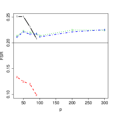
(a) False selection rate vs $p$

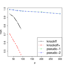
(b) True selection rate vs $p$

Figure 20: Logistic model; Performances under different dimensions at $\alpha=0.2$. Knockff and Knockoff+ method only work if $n>2p$.

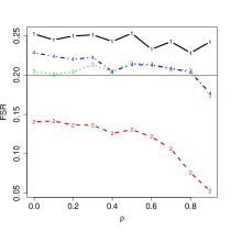
(a) False selection rate vs $\rho$

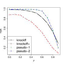
(b) True selection rate vs $\rho$

Figure 21: Logistic model; Performances under different correlations at $\alpha=0.2$.

(a) False selection rate vs $A$

(b) True selection rate vs $A$

Figure 22: Logistic model; Performances under different coefficient amplitude at $\alpha=0.2$.

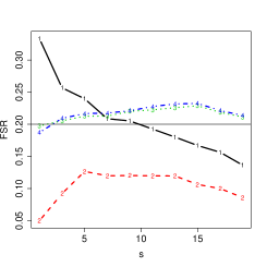
(a) False selection rate vs $s$

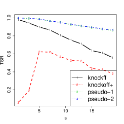
(b) True selection rate vs $s$

Figure 23: Logistic model; Performances under different number of nonzero coefficients at $\alpha=0.2$.

10 Simulation results for Cox model

In this section, the penalized Cox model is considered. Suppose the data are of the form $(Y_{i},X_{i},\delta_{i}),i=1,\ldots,n$, where $Y_{i}$ is the observed time, $X_{i}$ is covariate and $\delta_{i}$ is censoring indicator with $0$ means right-censoring and $1$ indicates failure. The Lasso estimator for Cox model at $\lambda$ is defined as

$$\widehat{\boldsymbol{\beta}}(\lambda;\mathbb{Y},\mathbb{X})=\arg\min_{\boldsymbol{\beta}\in\mathbb{R}^{p}}\left\{-\frac{1}{n}\sum_{i:\delta_{i}=1}^{n}\left[X_{i}^{\intercal}\boldsymbol{\beta}-\log\sum_{j:Y_{j}\geq Y_{i}}\exp(X_{j}^{\intercal}\boldsymbol{\beta})\right]+\lambda\sum_{j=1}^{p}|\beta_{j}|\right\}.$$

In the simulation, survival time $T_{i}$ follows a Weibull distribution with shape parameter 1 and scale $(0.01)\exp(X_{i}^{T}\boldsymbol{\beta}_{0})$. Censoring time $C_{i}$ is exponential distributed with mean $1000$. Similar to simulation study of penalized regression, we consider four settings: different predictor dimensions, correlation magnitudes, signal amplitudes, and number of nonzero coefficients. The censoring percentage are around $10\%$ to $35\%$ across different settings.

Simulation results are presented in Figure 24, 25, 26, and 27. A similar pattern as seen for penalized regression can be observed from those figures. In terms of TSR, the pseudo-variable methods and the knockoff method have better performances than the knockoff+, which is too conservative in some cases. Then for FSR, only the knockoff method exceeds the target error rate significantly.

Similar to implementation of knockoff and knockoff+ method for penalized logistic model, $create\_equicorrelated$ function is called first to construct knockoff variables, and glmnet function is called with family = cox to get when the original variables and knockoff enter the solution path. Signed maximum statistics are used for knockoff and knockoff+ method.

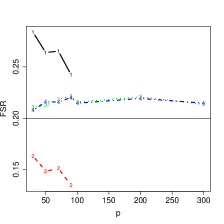
(a) False selection rate vs $p$

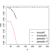
(b) True selection rate vs $p$

Figure 24: Cox model; Performances under different dimensions at $\alpha=0.2$. Knockff and Knockoff+ method only work if $n>2p$.

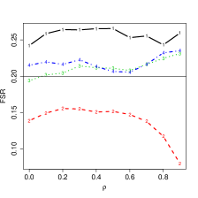
(a) False selection rate vs $\rho$

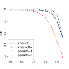
(b) True selection rate vs $\rho$

Figure 25: Cox model; Performances under different correlations at $\alpha=0.2$.

(a) False selection rate vs $A$

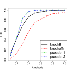
(b) True selection rate vs $A$

Figure 26: Cox model; Performances under different coefficient amplitude at $\alpha=0.2$.

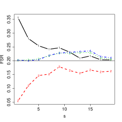
(a) False selection rate vs $s$

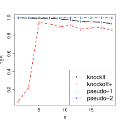
(b) True selection rate vs $s$

Figure 27: Cox model; Performances under different number of nonzero coefficients at $\alpha=0.2$.

11 Pseudo-variables algorithm for screening

In this section, we introduce a general algorithm for screening based on pseudo-variables. The intuition behind this algorithm is that the pseudo-variables can be used to assess the tuning parameter selected. Therefore, one can choose a tuning parameter that controls the percentage of pseudo-variables in the selected model. The Lasso estimator is defined as follows

$$\widehat{\boldsymbol{\beta}}(\lambda_{n};\mathbb{Y},\mathbb{X})=\arg\min_{\boldsymbol{\beta}\in\mathbb{R}^{p}}\left\{\frac{1}{2}||\mathbb{Y}-\mathbb{X}\boldsymbol{\beta}||^{2}+\lambda_{n}\sum_{j=1}^{p}|\beta_{j}|\right\},$$ (6)

where $\lambda_{n}$ is the tuning parameter. The detailed procedure for finding the tuning parameter is summarized as follows

• Step 0: Fix a sequence of lambda $\lambda_{(1)}<\lambda_{(2)}<\cdots<\lambda_{(m)}$

• Step 1: Generate $\mathbb{X}_{\mathrm{pseudo}}$ by direct permuting the rows of $\mathbb{X}$

• Step 2: Fit Lasso using $\mathbb{Y}$ and $\mathbb{X}_{\mathrm{all}}=(\mathbb{X},\mathbb{X}_{\mathrm{pseudo}})$, calculate $\widehat{A}_{\lambda_{(i)}}^{all}=\{j:\widehat{\boldsymbol{\beta}}_{j}(\lambda_{(i)};\mathbb{Y},\mathbb{X}_{\mathrm{all}})\neq 0\}$, then

  $$\widehat{p}_{\lambda_{(i)}}=\frac{\#\{j\in\widehat{A}^{all}_{\lambda_{(i)}}~{}\text{and $j$-th variable is pseudo}\}}{\max\left[\#\{j\in\widehat{A}^{all}_{\lambda_{(i)}}~{}\text{and $j$-th variable is not pseudo}\},1\right]}$$

• Step 3: Repeat Steps 1 and 2 $B$ times, and calculate $\widehat{p}_{\lambda_{(i)}}=1/B\sum_{b=1}^{B}\widehat{p}^{b}_{\lambda_{(i)}}$

• Step 4: Select tuning parameter $\widehat{\lambda}_{n}=\min\{\lambda_{(i)}:\widehat{p}_{\lambda_{(i)}}\leq\alpha_{n}\}$, where $\alpha_{n}$ is a constant.

After obtaining $\widehat{\lambda}_{n}$, one can then fit Lasso at $\widehat{\lambda}_{n}$ with $\mathbb{Y}$ and $X_{\mathrm{all}}=(\mathbb{X},\mathbb{X}_{pseudo})$. And then select those variables in the active set by excluding pseudo-variables. In the simulation studies, we fix $\alpha_{n}=0.2$ and $B=20$.

11.1 Theoretical properties

In this subsection, we prove that the algorithm above leads to consistent variable selection under certain conditions. Denote $\boldsymbol{\epsilon}=(\epsilon_{1},\ldots,\epsilon_{n})^{\intercal}.$ Denote $r_{n}\prec s_{n}$ if $r_{n}=o(s_{n})$, and $r_{n}\succ s_{n}$ if $s_{n}=o(r_{n})$. To prove the asymptotic consistency, we assume the following three conditions:

• There exists positive sequences $\{r_{n}\}$ and $\{s_{n}\}$ such that Lasso method with tuning parameter $\lambda_{n}$ is selection consistent whenever $r_{n}\prec\lambda_{n}\prec s_{n}$.

Use $\lambda_{n}^{*}$ to denote such a tuning parameter with $r_{n}\prec\lambda_{n}^{*}\prec s_{n}$. For such $\lambda_{n}^{*}$, then

$$P(\widehat{A}_{n}(\lambda_{n}^{*})=A_{0})\geq 1-k_{n},$$ (7)

for some $k_{n}\rightarrow 0$.

• For any $\tau>0$, there exists positive constant $c_{0}(\tau)$ and $n_{0}(\tau)$ such that, for $n>n_{0}(\tau)$, $P\left(\left\{\inf_{\tau r_{n}\leq\lambda\leq\lambda_{n}^{*}}\mathds{1}\left(\widehat{A}_{n}(\lambda)=A_{0}\right)\right\}=1\right)\geq 1-c_{0}(\tau),$ where $c_{0}(\tau)$ converges to zero as $\tau\rightarrow\infty$.

• For any pseudo variable $j$, and any $\tau>0$, there exists positive constant $c_{1}(\tau)$ and $n_{1}(\tau)$ such that, for $n>n_{1}(\tau)$, $P\left(\left\{\inf_{\lambda<\tau r_{n}}\mathds{1}\left(j\in\widehat{A}_{n}(\lambda_{n})\right)\right\}=1|\mathbb{X},\boldsymbol{\epsilon}\right)\geq c_{1}(\tau),$ almost surely.

For assumption (A3), when conditioning on $\mathbb{X}$ and $\boldsymbol{\epsilon}$, the randomness come from $\mathbb{X}_{\mathrm{pseudo}}$. Assumptions (A1) and (A2) have been verified in Sun et al. (2013). By similar argument as Sun et al. (2013), it is easy to verify assumption (A3) if assuming a strong condition that $\mathbb{X}_{\mathrm{pseudo}}$ are orthogonal to $\mathbb{X}$. Under above assumptions, we have the following theorem

Theorem 11.1.

Under Assumptions 1, 2 and 3, the tuning parameter $\widehat{\lambda}_{n}$ selected in the above algorithm leads to consistent variable selection, i.e., $\lim_{n\rightarrow\infty}\lim_{B\rightarrow\infty}P\left(\widehat{A}_{n}(\widehat{\lambda}_{n})=A_{0}\right)=1$ provided $1\succ\alpha_{n}\succ k_{n}$, where $k_{n}$ is defined in Eq. 7.

11.2 Proof of Theorem 11.1

Proof.

Define $S_{1}=\{\lambda:\lambda>\lambda_{n}^{*}\}$ and, $S_{2}=\{\lambda:\tau r_{n}>\lambda\}$. First, we show that for $\lim_{n\rightarrow\infty}P(\widehat{\lambda}_{n}\in S_{1}\cup S_{2})\rightarrow 0$. For $S_{1}$, by definition of $\widehat{\lambda}_{n}$ and $\lambda_{n}^{*}$, we have

$$P(\widehat{\lambda}_{n}\leq\lambda_{n}^{*}) \geq P(\widehat{p}_{\lambda^{*}_{n}}\leq\alpha_{n})$$

$$=1-P(\widehat{p}_{\lambda^{*}_{n}}>\alpha_{n})$$

$$\geq 1-\frac{E(\widehat{p}_{\lambda^{*}_{n}})}{\alpha_{n}}$$

$$=1-\frac{E(\widehat{p}^{b}_{\lambda^{*}_{n}})}{\alpha_{n}}$$

$$\geq 1-\frac{k_{n}}{\alpha_{n}}\rightarrow 1,$$

where the last inequality holds because of $E(\widehat{p}_{\lambda^{*}_{n}})\leq k_{n}$, which is implied by assumption A1. Therefore $\lim_{n\rightarrow\infty}P(\widehat{\lambda}_{n}\in S_{1})=0$.

Then for $S_{2}$, by the strong law of large numbers

$$\lim_{B\rightarrow\infty}\frac{1}{B}\sum_{b=1}^{B}\inf_{\lambda\in S_{2}}\widehat{p}_{\lambda}^{b}=E(\inf_{\lambda\in S_{2}}\widehat{p}_{\lambda}^{b}|\mathbb{X},\boldsymbol{\epsilon}).$$

And by Assumption A3, we know that for any pseudo variable $j$,

$$P\left(\left\{\inf_{\lambda<\tau r_{n}}\mathds{1}\left(j\in\widehat{A}_{n}(\lambda)\right)\right\}=1|\mathbb{X},\boldsymbol{\epsilon}\right)\geq c_{1}(\tau).$$

This implies

$$P\left(E(\inf_{\lambda\in S_{2}}\widehat{p}_{\lambda}^{b}|\mathbb{X},\boldsymbol{\epsilon})\geq c_{1}(\tau)/p\right)=1.$$

And since $\inf_{\lambda\in S_{2}}\widehat{p}_{\lambda}\geq B^{-1}\sum_{b=1}^{B}\inf_{\lambda\in S_{2}}\widehat{p}_{\lambda}^{b}$,

$$P\left(\inf_{\lambda\in S_{2}}\widehat{p}_{\lambda}\geq c_{1}(\tau)/p\right)=1-o(1).$$

This implies $\lim_{n\rightarrow\infty}P\left(\inf_{\lambda\in S_{2}}\widehat{p}_{\lambda}<\alpha_{n}\right)=0$. Therefore, $\lim_{n\rightarrow\infty}P(\widehat{\lambda}_{n}\in S_{2})=0$. So $\lim_{n\rightarrow\infty}P(\widehat{\lambda}_{n}\in S_{1}\cup S_{2})=0$, i.e., $\lim_{n\rightarrow\infty}P(\tau r_{n}\leq\widehat{\lambda}_{n}\leq\lambda_{n}^{*})=1$. Then,

$$P\left(\widehat{A}_{n}(\widehat{\lambda}_{n})=A_{0}\right) \geq P\left(\widehat{A}_{n}(\widehat{\lambda}_{n})=A_{0},\tau r_{n}\leq\widehat{\lambda}_{n}\leq\lambda_{n}^{*}\right)$$

$$\geq P\left(\left\{\inf_{\tau r_{n}\leq\lambda\leq\lambda_{n}^{*}}\mathds{1}(\widehat{A}_{n}(\lambda)=A_{0})\right\}=1\right)+P(\tau r_{n}\leq\widehat{\lambda}_{n}\leq\lambda_{n}^{*})-1.$$

Therefore by assumption A2, $\lim_{n\rightarrow\infty}\lim_{B\rightarrow\infty}P\left(\widehat{A}_{n}(\widehat{\lambda}_{n})=A_{0}\right)\geq 1-c_{0}(\tau)$. It holds for any $\tau$. Then let $\tau\rightarrow\infty$, we have $\lim_{n\rightarrow\infty}\lim_{B\rightarrow\infty}P\left(\widehat{A}_{n}(\widehat{\lambda}_{n})=A_{0}\right)=1$. ∎

References

- Barber and Candès (2015) Barber, R. F. and Candès, E. J. (2015). Controlling the false discovery rate via knockoffs. The Annals of Statistics, 43(5):2055–2085.
- Barber and Candès (2016) Barber, R. F. and Candès, E. J. (2016). A knockoff filter for high-dimensional selective inference. arXiv preprint arXiv:1602.03574.
- Chen and Chen (2008) Chen, J. and Chen, Z. (2008). Extended bayesian information criteria for model selection with large model spaces. Biometrika, 95(3):759–771.
- Efron (2012) Efron, B. (2012). Large-scale inference: empirical Bayes methods for estimation, testing, and prediction, volume 1. Cambridge University Press.
- Fan and Tang (2013) Fan, Y. and Tang, C. Y. (2013). Tuning parameter selection in high dimensional penalized likelihood. Journal of the Royal Statistical Society: Series B (Statistical Methodology), 75(3):531–552.
- Feng and Yu (2013) Feng, Y. and Yu, Y. (2013). Consistent cross-validation for tuning parameter selection in high-dimensional variable selection. arXiv preprint arXiv:1308.5390.
- Hall et al. (2009) Hall, P., Lee, E. R., and Park, B. U. (2009). Bootstrap-based penalty choice for the lasso, achieving oracle performance. Statistica Sinica, 19(2):449.
- Hui et al. (2015) Hui, F. K., Warton, D. I., and Foster, S. D. (2015). Tuning parameter selection for the adaptive lasso using eric. Journal of the American Statistical Association, 110(509):262–269.
- Meinshausen and Bühlmann (2010) Meinshausen, N. and Bühlmann, P. (2010). Stability selection. Journal of the Royal Statistical Society: Series B (Statistical Methodology), 72(4):417–473.
- Mezzadri (2006) Mezzadri, F. (2006). How to generate random matrices from the classical compact groups. arXiv preprint math-ph/0609050.
- Sabourin et al. (2015) Sabourin, J. A., Valdar, W., and Nobel, A. B. (2015). A permutation approach for selecting the penalty parameter in penalized model selection. Biometrics, 71(4):1185–1194.
- Shah and Samworth (2013) Shah, R. D. and Samworth, R. J. (2013). Variable selection with error control: another look at stability selection. Journal of the Royal Statistical Society: Series B (Statistical Methodology), 75(1):55–80.
- Stamey et al. (1989) Stamey, T. A., Kabalin, J. N., McNeal, J. E., Johnstone, I. M., Freiha, F., Redwine, E. A., and Yang, N. (1989). Prostate specific antigen in the diagnosis and treatment of adenocarcinoma of the prostate. ii. radical prostatectomy treated patients. The Journal of urology, 141(5):1076–1083.
- Sun et al. (2013) Sun, W., Wang, J., and Fang, Y. (2013). Consistent selection of tuning parameters via variable selection stability. Journal of Machine Learning Research, 14(1):3419–3440.
- Tibshirani (1996) Tibshirani, R. (1996). Regression shrinkage and selection via the lasso. Journal of the Royal Statistical Society. Series B (Methodological), pages 267–288.
- Wang et al. (2009) Wang, H., Li, B., and Leng, C. (2009). Shrinkage tuning parameter selection with a diverging number of parameters. Journal of the Royal Statistical Society: Series B, 71(3):671–683.
- Wu et al. (2007) Wu, Y., Boos, D. D., and Stefanski, L. A. (2007). Controlling variable selection by the addition of pseudovariables. Journal of the American Statistical Association, 102(477):235–243.
- Zhang et al. (2010) Zhang, Y., Li, R., and Tsai, C.-L. (2010). Regularization parameter selections via generalized information criterion. Journal of the American Statistical Association, 105(489):312–323.