A Mixture Model to Detect Edges in Sparse Co-expression Graphs

Abstract

In the early days of gene expression data, researchers have focused on gene-level analysis, and particularly on finding differentially expressed genes. This usually involved making a simplifying assumption that genes are independent, which made likelihood derivations feasible and allowed for relatively simple implementations. In recent years, the scope has expanded to include pathway and ‘gene set’ analysis in an attempt to understand the relationships between genes. We develop a method to recover a gene network’s structure from co-expression data, measured in terms of normalized Pearson’s correlation coefficients between gene pairs. We treat these co-expression measurements as weights in the complete graph in which nodes correspond to genes. To decide which edges exist in the gene network, we fit a three-component mixture model such that the observed weights of ‘null edges’ follow a normal distribution with mean 0, and the non-null edges follow a mixture of two lognormal distributions, one for positively- and one for negatively-correlated pairs. We show that this so-called $L_{2}N$ mixture model outperforms other methods in terms of power to detect edges, and it allows to control the false discovery rate. Importantly, the method makes no assumptions about the true network structure.

Keywords: covariance matrix, gene network, log-normal mixture model, EM algorithm.

1 Introduction

Broadly speaking, statistical analysis of ‘omics’ data consists of studying the relative abundance of biological ‘building blocks’, such as genes, proteins, and metabolites. The goal of many studies involving high-throughput data is to identify differential building blocks - those whose abundance levels vary according to the value of some other factor. These factors include, for example, environmental conditions, disease state, gender, or age. To simplify the discussion, we will use genomics terminology, where the building blocks are genes and the abundance is their expression level. Many biological studies use statistical methods which focus on individual genes and rely on the unrealistic, but mathematically convenient assumption that the expression levels are independent across genes. However, other methods drop this assumption and acknowledge that multiple genes are likely to work as a group associated with the same biological process, thus providing not only more complex functionality, but also robustness to detrimental mutations. A common assumption is that related genes share a regulatory process, and therefore, their expression levels are expected to be highly correlated. The relevant measurements in this context are co-expression levels of pairs of genes, which can be measured in terms of Pearson’s correlation coefficient, Mutual Information, Spearman’s rank correlation coefficient, or Euclidean distance. Gene co-expression data can be seen as a network; an undirected complete graph in which nodes represent genes and weights are assigned to edges according to the strength of the association between each pair’s expression levels, across multiple samples.

Using gene co-expression patterns, a number of authors defined ‘modules’ as sets of genes that have similar expression patterns; they then focused on a small number of intramodular ‘eigengenes’ or ‘hub genes’ instead of on thousands of genes [1, 2, 3, 4, 5]. Among them, the weighted gene co-expression network analysis (WGCNA, [2]) is a widely used approach. Among hub genes, the aforementioned independence assumption is more reasonable because genes belonging to different modules are expected to be much less correlated than genes within the same module. Thus, one can try to find differentially expressed hub genes with respect to a trait or treatment. However, methods assuming a specific structure and focusing on modules and their eigengenes or hub genes, are only suitable for certain networks where nodes within a module are highly connected but connections across modules are relatively rare. However, biological networks such as protein-protein and gene-gene interaction networks may have other network features where modules cannot be clearly partitioned. Such is the case, for example, with scale-free networks [6, 7, 8], a scale-free regime followed by a sharp cutoff [9, 10, 11], and other networks with curved degree distributions [12, 13, 14, 15]. Instead of identifying hub genes and comparing their differential expression levels between two traits or treatments, there have been other approaches that compare high dimensional covariance matrices between the two groups and identify risk genes based on the correlation structures [16, 17, 18, 19, 20]. Recently, Cai and Liu [19] suggested a method for large-scale testing of correlations under certain regularity conditions. Zhu et al. [20] suggested a sparse leading eigenvalue driven test that compares two high-dimensional covariance matrices obtained from schizophrenia and normal groups and identified novel schizophrenia risk genes. Such genes that are found to be highly associated with a trait or treatment are further analyzed by using knowledge-based pathway analysis tools such as Gene Set Enrichment Analysis (GSEA, [21, 22]). Pathway analysis differs from co-expression analysis in that it uses pre-defined gene sets (e.g., from the Gene Ontology (GO, [23]) or the Kyoto Encyclopedia of Genes and Genomes (KEGG, [24]). Such analyses help determine which pathways are over- or under-represented in the identified modules [25].

Obtaining accurate estimates of covariance (or precision) matrix is important for gene network analyses. However, it becomes challenging when the number of genes is larger than the sample size (as is often the case). The problem of estimating large, sparse gene networks has been thoroughly studied in modern multivariate analysis. Researchers have suggested various approaches using regularization techniques, and one of most commonly used approaches is the penalized maximum likelihood. For example, Meinshausen and Bühlmann [26] proposed to estimate a precision matrix by imposing an $l_{1}$ penalty on a Gaussian log-likelihood to increase its sparsity. It uses a simple algorithm to estimate a sparse precision matrix, by fitting a regression model to each variable with all other variables as predictors, and apply the lasso to obtain sparsity. Friedman et al. [27] suggested a simple but faster algorithm called graphical lasso, which also estimates a sparse precision matrix using coordinate descent procedure for lasso. Yuan and Lin [28], Banerjee et al. [29], Rothman et al. [30] and Levina et al. [31] also proposed algorithms to solve the $l_{1}$ penalized Gaussian log-likelihood to estimate a large, sparse precision matrix. These methods have been extensively used to estimate sparse gene network. The use of precision matrix for estimating gene network is justified when the data is generated from a multivariate normal distribution. Under this assumption, elements of the precision matrix correspond to conditional independence restrictions between nodes in a gene network. These approaches work well when analyzing gene data obtained from large retrospective studies such as the TCGA data [32]. However, applying these approaches to datasets with a relatively small number of samples may not yield robust estimates of the regression coefficients.

The main goal of this paper is to introduce a new method to uncover the structure of sparse gene networks from expression data. Rather than estimating the precision matrix, we use the covariance matrix to determine which genes are co-expressed. Sparsity in the covariance matrix (rather than the precision matrix) is motivated mostly by biological arguments – (i) expression level of genes are associated with their functionality, and thus, are expected to be highly correlated for genes that share the same functional process; and (ii) the number of genes associated with most biological functions is small, relative to the total number of genes. There is also a strong mathematical argument for modeling sparsity in the covariance matrix, rather than the precision matrix. For each gene, its expression profile is an $N$-dimensional vector where $N$ is the sample size, and for each pair of genes the correlation between their expression profiles represents the cosine of the angle between the two corresponding vectors. So, the correlation matrix offers an intuitive representation of the similarity between expression profiles. As Frankl and Maehara [33] showed, as $N$ increases, any two random vectors in the Euclidean $N$-dimensional space are approximately orthogonal with probability that approaches 1. Thus, the correlation between two random expression profiles is expected to be close to $cos(\pi/2)=0$, which means that the correlation (and hence, the covariance) matrix is expected to be sparse.

While gene expression datasets consist of thousands of genes and the complete network contains millions of edges, in most biological systems gene networks are expected to be sparse [34]. With a finite sample, however, the observed correlations are not zero, even for uncorrelated pairs, so the first problem is to define an accurate decision rule to differentiate between spurious correlations and true edges. A second, related problem, is how to perform the computation needed to implement such a rule in practice.

To address these challenges, we first obtain weights, $w_{ij}$, by applying Fisher’s Z transformation to the sample correlation coefficients, $r_{ij}$. For uncorrelated pairs, the asymptotic distribution of $w_{ij}$ is normal, with mean zero and variance $N-3$. This motivates fitting a mixture model to $\{w_{ij}\}$ in which the majority of pairs belong to a normally distributed ‘null component’, and a small percentage of the weights belong to one of two ‘non-null components’, which follow log-normal distributions (one for positive and one for negative correlations). This so-called $L_{2}N$ model was first presented in Bar and Schifano [35], in the context of identifying differentially expressed (or dispersed) genes. We use the $L_{2}N$ model to recover a sparse gene network for the following reasons. First, the $L_{2}N$ mixture model leads to shrinkage estimation and to borrowing strength across all pairs, which increases the power to detect co-expressed pairs. Second, the specific form of the mixture model allows us to establish a decision rule which controls the error rate. Third, the mixture model lends itself to a computationally-efficient estimation of the parameters via the EM algorithm [36]. Note that when Bar and Schifano [35] used the model, they assumed independence between genes, while this is not the case in our application. Furthermore, they used the $L_{2}N$ model in the k-group comparison setting, while in our application we fit the model to detect a network for each group.

This paper is organized as follows: in Section 2 we present our method to uncover the structure of gene networks. We discuss some computational challenges and our proposed solutions. In Section 3 we evaluate the goodness of fit of our method and its ability to correctly recover the network structure and compare our method’s ability to correctly identify true edges with existing methods. In Section 4 we apply our method to a publicly available collection of breast cancer datasets from twelve studies. We conclude with a discussion in Section 5.

2 Statistical Model and Estimation

2.1 A Mixture Model for Edge Indicators in a Gene Network

A gene network can be represented by a weighted, undirected graph in which each node corresponds to a gene and each edge corresponds to a pair of genes that are ‘co-expressed’, meaning that their expression levels are highly correlated. The weights represent the strength of the connection between two genes, namely, their tendency to be co-expressed. Given normalized expression data of $G$ genes, our objective is to discover the network structure, namely, which of the $K=G(G-1)/2$ pairs are co-expressed. Our general strategy is to associate with every putative edge in the complete graph with $G$ nodes, a latent indicator variable whose value (0 or 1) is determined by a statistical model.

To start, we define the edge weights in terms of pairwise correlation coefficients. Let $\mathbf{x}_{g}$ be a vector of normalized expression levels for gene $g\in\{1,\ldots,G\}$ obtained from $N$ samples ($N>3$). Suppose that the true correlation coefficient between genes $m$ and $n$ is $\rho_{mn}$, and let $r_{mn}=corr(\mathbf{x}_{m},\mathbf{x}_{n})$ be the observed correlation coefficient. Using Fisher’s Z transformation, we obtain the estimated weight $w_{mn}=arctanh(r_{mn})$, which is known to be approximately normally distributed, with mean $arctanh(\rho_{mn})$ and variance $\frac{1}{N-3}$. Let $E=\{e_{mn}\}$ be the set of true edges in the network. We assume that $G$ is large and that most pairs are not co-expressed, so the network is sparse: $|E|\ll K$. This assumption, along with asymptotic normality of $w_{mn}$, motivate our model choice. Specifically, we assume that the weights follow the so-called $L_{2}N$ mixture distribution in Bar and Schifano [35]. $L_{2}N$ is a three-component mixture model in which the ‘null’ component follows a normal distribution with mean 0, representing the majority of pairs that have approximately zero correlation, and the tails (the ‘non-null’ components, for pairs with strong positive/negative correlations) follow log-normal distributions:

$$w_{mn}|e_{mn}\notin E \sim N(0,\sigma^{2})$$ (1)

$$w_{mn}|[w_{mn}>0,\,e_{mn}\in E]\, \sim LogNormal(\theta_{1},\kappa_{1}^{2})\,,$$ (2)

$$\vspace*{-10pt}-w_{mn}|[w_{mn}<0,\,e_{mn}\in E]\, \sim LogNormal(\theta_{2},\kappa_{2}^{2})\,.\vspace*{-10pt}$$ (3)

Note that $\sigma^{2}$ consists of two variance components, namely, $\sigma^{2}=\frac{1}{N-3}+\sigma_{0}^{2}$, where $\frac{1}{N-3}$ is the variance component due to the asymptotic distribution of $arctanh(r_{mn})$, whereas $\sigma_{0}^{2}$ is due to the random effect model, which allows us to account for extra variability among uncorrelated pairs. A graphical representation of the $L_{2}N$ model is shown in Figure 1.

If we denote the null mixture component in the $L_{2}N$ model by $C_{0}$, the two non-null components by $C_{1}$ and $C_{2}$, the corresponding probability density functions by $f_{j}$, and the mixture probabilities by $p_{j}$, for $j=0,1,2$, such that $p_{0}+p_{1}+p_{2}=1,$ then we classify a putative edge between nodes $m$ and $n$ in the complete graph into one of the three mixture components based on the posterior probabilities,

$$Pr(e_{mn}\in C_{j}|w_{mn})=\frac{p_{j}f_{j}(w_{mn})}{p_{0}f_{0}(w_{mn})+p_{1}f_{1}(w_{mn})+p_{2}f_{2}(w_{mn})},\leavevmode\nobreak\ j=0,1,2.$$ (4)

Let $\mathbf{b}_{mn}=(b_{0mn},b_{1mn},b_{2mn})$ be an indicator vector, so that $b_{jmn}=1$ for the component $j$ with the highest probability, $Pr(e_{mn}\in C_{j}|w_{mn})$, for the pair $mn$, and 0 for the other two components. Using this notation, the $G\times G$ matrix $\textbf{A}=[1-b_{0mn}]$ denotes the adjacency matrix between the $G$ nodes in the graph. Our goal is to obtain an accurate estimate of A. To do that, we treat the indicators $\mathbf{b}_{mn}$ as missing data, and use the EM algorithm [36] to estimate the parameters of the mixture model. The hierarchical and parsimonious nature of the $L_{2}N$ model leads to shrinkage estimation and borrowing power across all pairs of genes, as well as to computational efficiency. This is critical, since $K$ is typically very large and can be much larger than the sample size, $N$. Details regarding the parameter estimation for the $L_{2}N$ model can be found in [35]. The algorithm is implemented as an R-package called edgefinder (see the Supplementary Material).

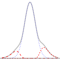
Figure 1: The $L_{2}N$ mixture model, with probability of the null component (blue dotted curve), $Pr(mn\in C_{0})=0.8$, where $mn$ denotes the edge between nodes $m$ and $n$ in the graph.

2.2 Implementation Notes

There are a couple of challenges related to the parameter estimation via the EM algorithm which should be addressed. First, the complete set of pairwise correlation coefficients, and thus the normalized weights, $w_{mn}$, cannot be assumed to be mutually independent. Conditionally, they are all asymptotically normally distributed with variance $\frac{1}{N-3}$, but for a fixed $m$, some $w_{mn}$ may be correlated. Second, obtaining estimates based on all $K$ pairwise correlations is time-consuming and requires storing a very large matrix in the computer’s memory, since the values of the indicator variables, $\hat{b}_{jmn}$, for each pair of genes must be updated in each iteration of the EM algorithm.

When the number of genes is large, as is the case in the applications which motivated this paper, we propose taking a random sample of $G^{\prime}<G$ genes (e.g., $G^{\prime}=1000$) and fitting the mixture model to this random subset. Using the smaller subset of genes greatly improves computational efficiency and yields highly accurate estimates. Furthermore, randomly selecting a subset of the genes allows us to assume that the remaining weights used in the (complete data) likelihood function are approximately independent. With the estimates obtained from the random subset, it is then possible to compute the posterior probabilities (4) for all $K$ pairs, even on a computer with standard memory capacity.

In addition to computational efficiency and increasing power through shrinkage estimation, the mixture model allows us to estimate how many pairs of genes are correctly (or incorrectly) classified as co-expressed. Specifically, for a predetermined posterior probability ratio threshold, $T>1$, we solve

$$c_{1}=\arg\min_{w\in(0,\infty)}\frac{\hat{p}_{1}\hat{f}_{1}(w)}{\hat{p}_{0}\hat{f}_{0}(w)}>T\text{ \kern 10.00002ptand \kern 10.00002pt}c_{2}=\arg\max_{w\in(-\infty,0)}\frac{\hat{p}_{2}\hat{f}_{2}(w)}{\hat{p}_{0}\hat{f}_{0}(w)}>T$$

and set $b_{0mn}=1$ if $w_{mn}\in[c_{2},c_{1}]$, and $b_{0mn}=0$ otherwise. Alternatively, for any $\alpha$, we can (numerically) find thresholds $c_{1}>0$ and $c_{2}<0$ such that

$$Pr(\hat{b}_{0mn}\neq 0\leavevmode\nobreak\ |\leavevmode\nobreak\ b_{0mn}=0) \approx \hat{p}_{0}\int_{-\infty}^{c_{2}}\hat{f}_{0}(w)dw+\hat{p}_{0}\int_{c_{1}}^{\infty}\hat{f}_{0}(w)dw\leq\alpha\,.$$ (5)

That is, we control the estimated probability of a Type I error at a certain level, $\alpha$. Similarly, we can control the false discovery rate [37]. Using the thresholds $c_{1}$ and $c_{2}$, we can estimate the probability of a Type II error:

$$Pr(\hat{b}_{0mn}=0\leavevmode\nobreak\ |\leavevmode\nobreak\ b_{0mn}\neq 0) \approx \hat{p}_{2}\int_{c_{2}}^{0}\hat{f}_{2}(w)dw+\hat{p}_{1}\int_{0}^{c_{1}}\hat{f}_{1}(w)dw.$$ (6)

3 Simulation Study

3.1 Data Generated Under the $L_{2}N$ Model

In the first simulation study, we assess the power and goodness of fit of our model using different configurations, with varying numbers of genes (G), samples (N), degrees of sparsity ($p_{1}+p_{2}$), and graph structures. In this section, data are generated according to the $L_{2}N$ model from Section 2, and we use different parameters for the log-normal components. We show representative results with $N=100$ and $G=500$ (thus, $K$, the maximum possible number of edges is 124,750.) Four network configurations are used in this section. They are described in terms of the shape of the $G\times G$ adjacency matrix, $A$, as follows:

• complete: $A=BlockDiag(J_{S}-I_{S},0_{G-S})$, where $S=100$, $J$ is a matrix of 1’s, $I$ is an identity matrix, and $0$ is a matrix of zeros. This graph contains one clique (complete subgraph) with 100 nodes, and nodes not in the clique are not connected to other nodes. $|E|=4,950$ ($\approx 0.04K$), $p_{1}=0.0396$, $p_{2}=0$.

• ar (autoregressive): $A$ has a Toeplitz structure, with $A_{ij}=1/(1+|i-j|)$ if both $i,j\leq S$, where $S=100$. $|E|=4,950$, $p_{1}=0.0396$, $p_{2}=0$.

• two independent blocks: $A=BlockDiag(J_{S}-I_{S},J_{S}-I_{S},0_{G-2S})$, where $S=50$. (I.e., two distinct cliques, each with 50 genes.) $|E|=2,450$, $p_{1}=0.0196$, $p_{2}=0$.

• two negatively correlated blocks: Similar to the previous configuration, but the two blocks are negatively correlated. $|E|=4,950$, $p_{1}=0.0196$, $p_{2}=0.02$.

For pairs $i,j$ such that $A_{ij}=0$, we generated $w_{ij}$ independently from a standard normal distribution. In the complete and two independent blocks configurations, for $A_{ij}=1$ we generated only positively correlated pairs (so $p_{2}=0$), and in the two negatively correlated blocks configuration, the pairs were positively correlated within each block, but pairs across the two blocks were generated to be negatively correlated. For the ar structure, weights generated from the log-normal distribution appear in the off-diagonals of $A$ in decreasing order. That is, the largest $G-1$ weights are placed randomly in the secondary diagonal (elements $A_{i,i+1}$), the next $G-2$ largest weights are placed randomly in the ternary diagonal (elements $A_{i,i+2}$), etc. (Note that the values $A_{ij}$ in this case are only used to indicate that elements along diagonals are equal, but these values are not used to generate the weights.)

All four configurations are sparse, with only 2-4% of the putative edges being present in the graph. The two negatively correlated blocks structure has the same sparsity as the complete and ar graphs, but it has different weights of non-null mixture components. The ar graph has a more constrained structure, with weights among pairs of nodes which decay as $|i-j|$ increases, for $i,j\leq S$. Recall, however, that our method does not rely on any assumptions about the structure of the graph. Therefore, it is expected that its performance will only depend on the parameters involved in the mixture model. In the simulations presented here we examined the power of the method to detect edges in the graphs as a function of the location parameters of the log-normal components. We varied $\theta_{1}$, such that $\theta_{1}\in\{-1.25,-1,-0.75,\ldots,0.75\}$, and set $\kappa_{1}^{2}=0.25$. In the two negatively correlated blocks configuration, we used $\theta_{2}=\theta_{1}$ and $\kappa_{2}=\kappa_{1}$. The weights which were generated according to the $L_{2}N$ model were transformed into correlation coefficients using the $\tanh$ function, and the resulting covariance matrix was used to simulate 500 gene expression values for 100 subjects. For each configuration we generated 20 different datasets.

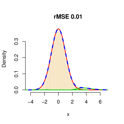
Figure 2: The distribution of $w_{mn}=arctanh(r_{mn})$ for a simulated dataset with 500 genes, of which 100 form a complete subgraph. The total number of edges in the graph is 4,950 (out of a total of 124,750 possible edges.) The red curve represents the null component, the green curves represent the non-null components, and the dashed blue line represents the fitted mixture distribution.

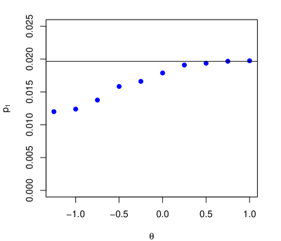
Figure S1: The average estimate of $p_{1}$, the proportion of positively correlated pairs of genes, from 20 replications, is plotted versus $\theta$ in the two negatively correlated blocks configuration. The horizontal black line depicts the true value of $p_{1}$.

We applied our method and checked the goodness of fit of the mixture model and the ability to correctly recover the structure of the network, in terms of the number of true- and false-positive edges. In our simulations, we used the approach described in Section 2 to control the false discovery rate at the 0.01 level. To demonstrate how well our algorithm estimates the true mixture model, we plotted for each configuration the histogram of the observed $w_{mn}$ and the fitted mixture and measured the goodness of fit in terms of the root means squared error (rMSE). In all configurations, the rMSE was very small ($\leq 0.01$), and the mixture weights ($p_{0}$, $p_{1}$, $p_{2}$) were estimated very accurately and with increasing accuracy as $\theta_{1}$ increases. See, for example, Figure S1 in the supplementary material, where the average estimate of $p_{1}$ is plotted versus $\theta$ using the two negatively correlated blocks configuration. A representative goodness of fit plot is shown in Figure 2, for the complete configuration, with $\theta_{1}=-0.25$. The red curve represents the null component, the green lines represent the non-null components (in this case, $C_{2}$ is estimated, correctly, to have a weight which is very close to 0), and the dashed blue line is the mixture.

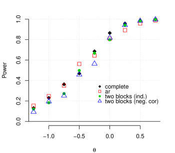
Figure 3: The average power of our method when the data are generated according to the $L_{2}N$ mixture model, as a function of $\theta$, for a simulated dataset with 500 genes and four different forms of adjacency matrices (complete, autoregressive, two independent blocks, and two negatively correlated blocks). In all cases, the FDR was controlled at the 0.01 level.

Arguably, more important than assessing goodness of fit, is determining a method’s ability to recover the true network structure correctly, i.e. identify as many existing edges as possible while maintaining a low number of falsely-detected edges. Figure 3 shows the average power of our method to detect true edges for a range of values for $\theta_{i}$ (with a fixed $\kappa^{2}$) and for different network configurations, where power is the total number of true-positives divided by the total number of edges in the graph. It can be seen that, as the location parameter of the log-normal distribution increases, the power increases and approaches 1. When the data are generated under the $L_{2}N$ model, this is the expected behavior, since as $\theta_{1}$ ($\theta_{2}$) increases, the positive (negative) non-null component, $C_{1}$ ($C_{2}$), is pushed further to the right (left), making it easier to discriminate between non-null and null components. Note that our method has approximately the same power curve for all four configurations.

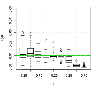
Figure S2: The observed false discovery rate in the simulations under the $L_{2}N$ model (Section 3.1), as a function of the location parameter of the log-normal distributions of the non-null components. The green horizontal line shows the level (0.01) which we used to control the false discovery rate. Using the notation Section 2, we determined the thresholds, $c_{1}$ and $c_{2}$, that correspond to this FDR level. The boxplots show the distributions across four network structures, with 20 replications in each configuration.

The average false discovery rate across all configurations and replications is 0.008. For small values of $\theta_{1}$ ($<-0.75$), the average FDR is slightly higher (approximately 0.012) and for $\theta>0$, the average FDR is less than 0.01. More detailed results regarding the achieved false discovery rate are shown graphically in Figure S2.

3.2 Data Generated Under Other Models

In the second simulation study we evaluate the ability of our method to recover the true network structure and compare it with other methods. For a fair comparison, the data are not generated under $L_{2}N$ model. Rather, we use data generated from a multivariate normal distribution whose covariance matrix $\Sigma$ is defined as a function of an adjacency matrix $A$. To generate data, we use the R-package huge [38]. We generate five types of network configurations as follows:

• random: each edge is randomly set to exist in the graph using $K$ i.i.d. Bernoulli(p) draws ($p=0.01,0.05,0.1$). $|E|\approx 1000\times(1000-1)\times p/2$.

• hub: it consists of $g$ disjoint groups, and nodes within each group are only connected through a central node in the group ($g=25,50,100$). $|E|=1000-g$.

• band: an edge, $e_{mn}$ between nodes $m\neq n$ is set to exist in the graph if $1\leq|m-n|\leq g$ ($g=25,50,100$). $|E|=(2000-1-g)\times g/2$.

• scale-free: scale-free networks are generated using the Barabási-Albert algorithm [39]. $|E|=1,000$.

• overlapped-cluster: we modified a function that generates a cluster network that consists of non-overlapping $g$ groups. In the modified function, the groups are aligned in an adjacency matrix so that each group shares 20% of the nodes with its left-adjacent group and another 20% with its right-adjacent group. Edges in each group are randomly generated with probability $p$. We use $p=0.3$ for $g=25$ and $50$, and $p=0.6$ for $g=100$. $|E|\approx(0.8\times(g-1)+1)\times(1000/g)\times(1000/g-1)\times p/2$. Edges in each group are randomly generated with probability $p$.

For each configuration, we generated expression profiles of $G=1,000$ genes for $N=70$ samples. We compare our method with three existing methods: Meinshausen-Bühlmann graph estimation (MB, [26]), graphical lasso (glasso, [27]), and correlation thresholding graph estimation. For each of MB and glasso, we identify edges in two different ways. First, an edge $e_{mn}$ between nodes $m$ and $n$ is estimated to exist (i.e. $\hat{A}_{mn}=1$) if the method chooses the node $m$ as a neighbor of $n$ and the node $n$ as a neighbor of $m$, which we name as MB-AND and glasso-AND, respectively. Second, an edge $e_{mn}$ is estimated to exist if the method chooses the node $m$ as a neighbor of $n$ or the node $n$ as a neighbor of $m$, which we name as MB-OR and glasso-OR, respectively. The sparsity levels of MB and glasso are controlled by a regularization parameter $\lambda$ and the correlation thresholding method by setting different thresholds from 0 to three times the true sparsity level.

We compare the performance in terms of the number of true positives (i.e. correctly identified edges) given the same total number of edges identified. We define the true network in two different ways: (i) based on the adjacency matrix — a pair $m,n$ is set to be connected if and only if $A_{mn}=1$, and (ii) by applying a threshold to the true covariance matrix — for a predetermined $t$, a pair is connected iff $|\Sigma_{mn}|>t$ where the threshold $t$ is set to achieve the same sparsity level as that of the adjacency matrix. The two are different in that the former assumes conditional independence between two nodes that not connected by an edge, while the latter does not.

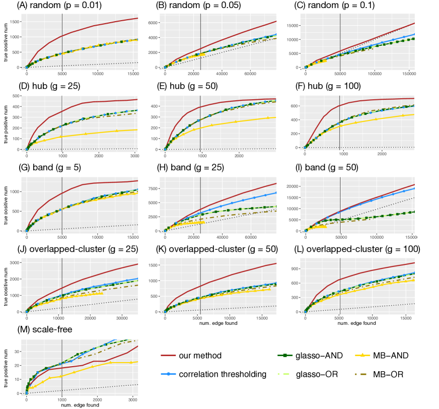
Figure S3: The numbers of true positive edges given the total number of edges identified by each method. The true matrix is obtained by applying a threshold to the true covariance matrix. The y-axis represents the number of true positive edges and the x-axis represents the total number of edges identified. The vertical line represents the number of true edges. The black dotted line is a regression line with 0 intercept and slope equal to the true sparsity, which represents the expected number of true positive edges when the edges are identified in a random manner.

The results from the two network definitions are similar. We show the result from (i) whose true matrix is derived from the adjacency matrix, and show the result from (ii) whose true matrix is derived from the true covariance matrix in the supplementary material (Figure S3).

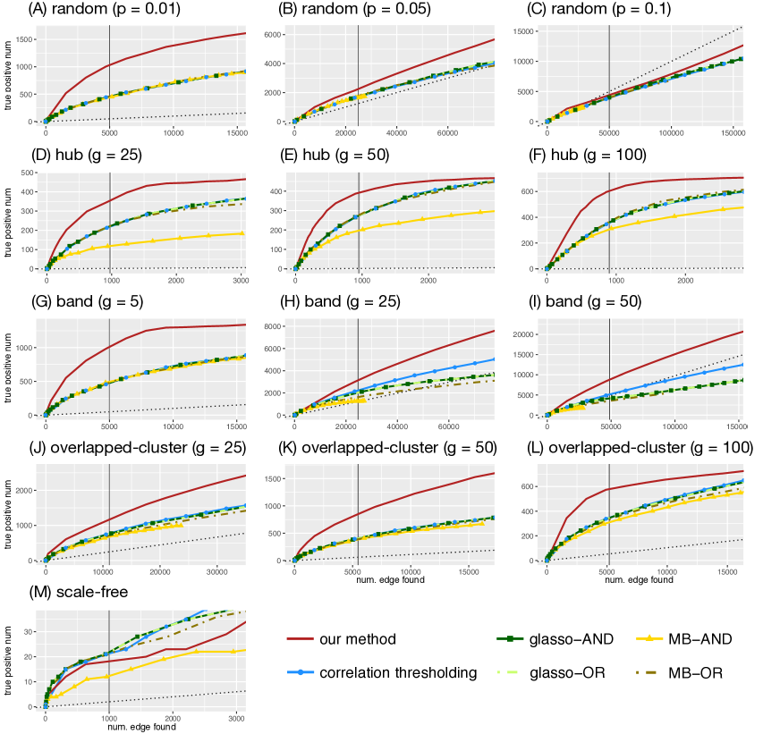
Figure 4: The numbers of true positive edges given the total number of edges identified by each method. The adjacency matrix used by the huge package is used to determine the true edges. The y-axis represents the number of true positive edges and the x-axis represents the total number of edges identified. The vertical line represents the number of true edges. The black dotted line is a regression line with 0 intercept and slope equal to the true sparsity, which represents the expected number of true positive edges when the edges are identified in a random manner (uniformly).

Figure 4 depicts the numbers of true positive edges given the total number of edges identified by each method. Our method (solid red lines) outperforms all the other methods in random, hub, band, and overlapped-cluster networks (see Figure 4A-L). For example, in the hub, $g=100$ configuration (panel F), the true number of edges is 900 (as indicated by the vertical line), and when our method detects 853 edges, 595 of them are true edges. In contrast, the thresholding method yields approximately 345 true edges out of the total 856 detected; MB-OR and glasso- yield approximately 370–380 true edges out of 900–960 edges detected; and MB-AND yields 312 true edges out of 930 edges detected. Notably, MB and glasso are comparable to, but in some cases worse than the correlation thresholding method in all network configurations.

The black dotted line in each plot represents the expected number of true positive edges when the edges are identified in a random manner. In the band, $g=50$ configuration (panel I), the competing methods do as well as or worse than chance, whereas our method gives much better results. In the random, $p=0.1$ configuration (panel C), the other methods perform worse than choosing edges randomly and our method performs slightly better than chance to a certain point (approximately 30,000 total edges being detected) before deteriorating, but still gives better results than the other methods.

The scale-free configuration appears to be especially challenging for all the methods. They all detect only approximately 10 – 20 true edges when the total number of edges detected was 1,000 (Figure 4M). In this case, the correlation thresholding, glasso- and MB-OR perform only slightly better than our method.

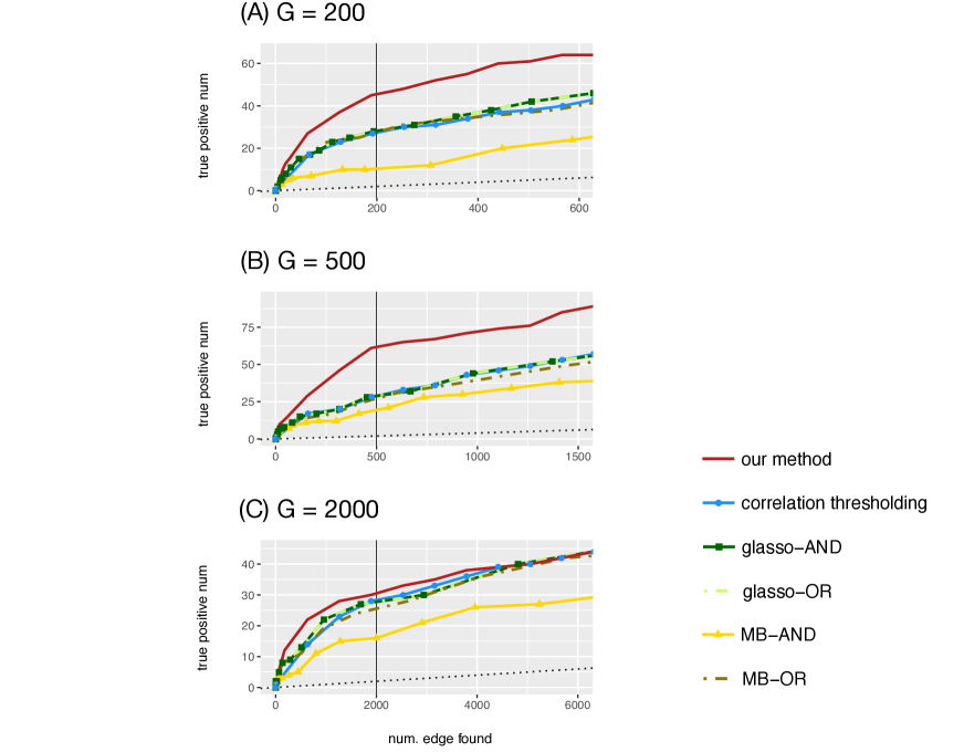
Figure S4: The numbers of true positive edges given the total number of edges using three scale-free network configurations ($G=200,500,2000$, where $G$ is the number of genes). The adjacency matrix is used as the true matrix. The y-axis represents the number of true positive edges and the x-axis represents the total number of edges identified. The vertical line represents the number of true edges. The black dotted line is a regression line with 0 intercept and slope equal to the true sparsity, which represents the expected number of true positive edges when the edges are identified in a random manner.

We further explore scale-free networks with additional network sizes ($G=200,500,2000$). Consider that sparsity levels change as we vary the network sizes: larger $G$ results in a more sparse network. Figure S4 depicts the numbers of true positive edges given the total number of edges for various sizes of scale-free networks. When $G=2,000$, our method is much better than MB-AND (as we have also seen in Figure 4M), and slightly better than the other methods. However, when $G=200,500$, our model outperforms the other methods. For example, when $G=200$, our model identifies around 45 true edges out of 200 edges, while glasso-, MB-OR, and the correlation thresholding methods identify less than 30 true edges, and MB-AND identifies around 10 edges.

4 Case Study

Subtype Characterization of Breast Cancer. We analyzed a large dataset used by Allahyar et al. [40] who introduced SyNet, a computational tool aiming to improve network-based cancer outcome prediction. The dataset, referred to as ACES [41], contained expression data for 12,750 genes collected from 1,616 women across 12 studies. To obtain and preprocess the data, we used the raw data and scripts provided by Allahyar et al. [40] via their github page (github.com/UMCUGenetics/SyNet). We focused on analyzing gene networks by cancer subtype: Basal (n=297), Her2 Positive (n=191), Luminal A (n=584), Luminal B (n=440), and Normal (n=104). Categorization into breast cancer types is based on the positive/negative status of three factors: estrogen receptor (ER), progesterone receptor (PR), and the number of copies of the HER2 gene. The Basal group is called the triple-negative breast cancer, and it includes tumors in which all three markers (ER, PR, HER2) are negative. The Her2 group includes tumors that are ER and PR negative, but HER2 positive. The Luminal A group includes tumors that are ER positive and PR positive, but HER2 negative. The Luminal B group includes tumors that are ER positive, PR negative, and HER2 positive.

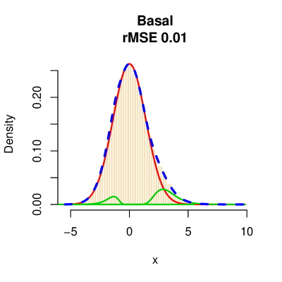
Figure S5: Goodness of fit plot of $L_{2}N$ mixture model. The distributions of $w_{mn}=arctanh(r_{mn})$ for the Basal group. The red curve represents the null component, the green curves represent the nonull components, and the dashed blue line represents the fitted mixture distribution.

We selected 80 random samples from each group, and applied edgefinder to detect the edges in the network in each of the five groups. We controlled the false discovery rate at the 0.01 level. With 12,750 genes there are 81,274,875 possible edges in the network, and edgefinder detects 112,071 edges in the network of the Normal group, 171,959 in the Basal group, 144,128 in the Her2 group, 278,066 in Luminal A, and 213,200 in Luminal B. Clearly, all five networks are very sparse (0.1-0.3% sparsity). All but two edges (in the Basal network) belonged to the positive correlation component in the mixture model. The results are very stable, in the sense of Meinshausen and Bühlmann [26], so that when we picked 100 different subsamples from each subtype, the same edges were detected in each of the cancer groups, and in the normal group the same network was detected 99 times. The mixture model for the normalized correlation coefficients fits all five very well, with rMSE=0.01. For example, Figure S5 in the Supplementary Material shows the fitted curve for the Basal group.

We now consider two characteristics of nodes, namely the degree, $d_{m}$, and the clustering coefficient, $\gamma_{m}$, where $m$ indicates a node $m$. Let $N_{m}=\{n\leavevmode\nobreak\ |\leavevmode\nobreak\ A_{mn}=1\}$ be the set of nodes adjacent to node $m$, and let $E(N_{m})$ be the set of edges between nodes in $N_{m}$. Then

$$d_{m}=|N_{m}|\text{ \kern 10.00002ptand \kern 10.00002pt}\gamma_{m}=\frac{|E(N_{m})|}{d_{m}(d_{m}-1)/2}\,.$$

If $d_{m}\leq 1$, the clustering coefficient is defined as $\gamma_{m}=0$. By definition, $\gamma_{m}\in[0,1]$. The degree of a node is interpreted as the involvement of the node in the network and the clustering coefficient as the connectivity among neighbors of the node. Note that $\gamma_{m}d_{m}$ is, by definition, proportional to $|E(N_{m})|/(d_{m}-1)$, so it is interpreted as (approximately) the average degree among the neighbors of node $m$. Note also that $\gamma_{m}d_{m}$ is bounded by $d_{m}$. To visualize and compare the properties of the networks, we plot $\gamma_{m}d_{m}$ versus $d_{m}$. For example, Figure 5 depicts the relationship between the degree and the clustering coefficients of nodes for (a) the Normal group and (b) the Her2 group. Similar plots for the other three subtypes are provided in the Supplementary Material. In all five groups we observe that as the degree of a node increases, the average degree of each of its neighbors increases. The plot for the Her2 group has a striking pattern, with three distinct ‘arms’, one of which exhibits a very high degree of connectivity between nodes (as shown by the high values of $\gamma_{m}d_{m}$.) This suggests that there is at one cluster which is nearly a complete subgraph in which each node is connected to all or most other nodes in that cluster. The presence of such clusters is also depicted in Figure 6, which shows a bitmap of the data (restricted to genes with at least 20 neighbors), where a black dot represents an edge between a pair of nodes and white dots represent pairs which are not connected. To detect clusters and to generate plots such as Figure 6, where clusters are arranged by their size, we first define the dissimilarity between two neighboring nodes, $m$ and $n$, as the number of neighbors of $m$ which are not neighbors of $n$, plus the number of neighbors of $n$ which are not neighbors of $m$. Then, we create clusters recursively as follows. In each iteration, $i$, we find the node, $x_{i}$, with the largest degree and identify all of its neighbors. We sort its neighbors in increasing dissimilarity order. So, within the $i$-th cluster, the nodes are arranged from closest to $x_{i}$ to the farthest. Then, in the subsequent iterations node $x_{i}$ and all its neighbors are excluded, until we have exhausted all the nodes.

Figure 6 shows that the genes in the second largest cluster in the Her2 network appear to be highly connected. Figure 7 shows again the plot of $\gamma_{m}d_{m}$ versus $d_{m}$, but this time, genes identified as belonging to the second largest cluster appear in red. Clearly, the upper ‘arm’ in the plot consists of genes from that cluster.

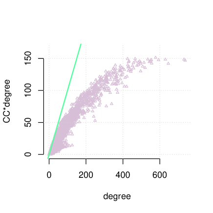
(a) Normal

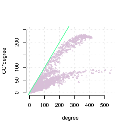
(b) Her2

Figure 5: Plot of $\gamma_{m}d_{m}$ versus $d_{m}$, where $\gamma_{m}$ is the clustering coefficient and $d_{m}$ is the degree of node $m$.

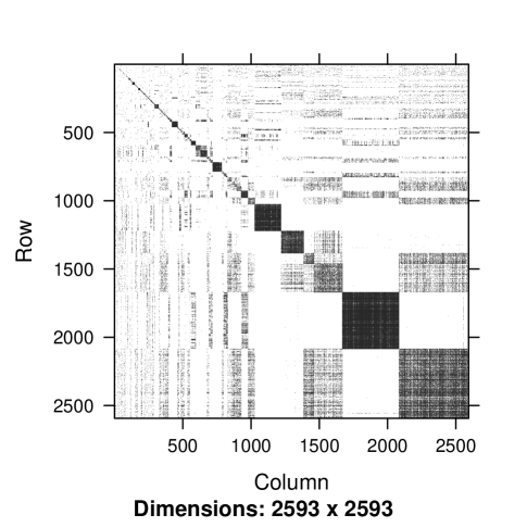
Figure 6: A bitmap of the Her2 network, including only genes with at least 20 neighbors. A black dot represents an edge between a pair of nodes, and white dots represent pairs which are not connected. The genes were ordered according to their degree, within each cluster.

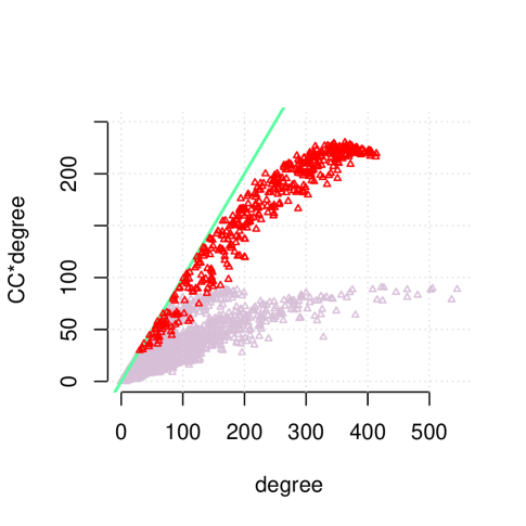
Figure 7: Plot of $\gamma_{m}d_{m}$ versus $d_{m}$ for the Her2 group. Points in red correspond to genes identified as belonging to the second largest cluster.

Table 1: Pathways characterizing the breast cancer subtypes.

Subtype Pathway Name Pathway Size Cluster Index P-value Genes Her2 Steroid hormone biosynthesis 42 18 0.000780 AKR1C1, AKR1C2, HSD3B1, SRD5A1, AKR1D1, UGT2B28 Tryptophan metabolism 35 18 0.002258 KYAT1, DDC, MAOA, KYNU, HAAO Drug metabolism - cytochrome P450 54 18 0.009187 ADH1C, CYP2A6, FMO5, MAOA, UGT2B28 Basal RNA transport 126 46 0.004090 CLNS1A, RAN, RANBP2, NUP160, SUMO4 mRNA surveillance pathway 68 70 0.004276 PPP2CA, PPP2R5C, PPP2R5E, PPP2R3C LumA Bacterial invasion of epithelial cells 65 3 0.006240 CAV1, CAV2, HCLS1, ILK, ITGA5, PIK3CD, ELMO1, ARPC1B Lum B Tight junction 118 39 8.34E-05 ACTN2, ACTN3, MYH1, MYH2, MYL2, MYLPF Base excision repair 31 37 0.001882 FEN1, PCNA, UNG Dilated cardiomyopathy 83 42 0.002040 MYL2, TNNC1, TPM3, TTN Hypertrophic cardiomyopathy (HCM) 77 42 0.002040 MYL2, TNNC1, TPM3, TTN Regulation of autophagy 30 3 0.003573 IFNA4, IFNA10, IFNA17, IFNA21 Nucleotide excision repair 41 37 0.003760 PCNA, RFC4, RFC5 • Uniquely enriched pathways in each breast cancer subtype. All identified clusters are indexed by their size. The cluster index indicates the order of the clusters. P-values are adjusted to control the false discovery rate using Benjamini and Hochberg [37].

Next, we characterize each subtype by pathways enriched in its gene clusters. For each subtype, we perform gene set enrichment analysis [21] and find the KEGG pathways significantly enriched in every identified cluster (p-value $\leq 0.01$). We then identify uniquely enriched pathways for each subtype compared to other subtypes (see Table 1).

Our results obtained from the pathway analysis are consistent with the previous findings. The HER2 group has three uniquely enriched pathways: drug metabolism–cytochrome P450, steroid hormone biosynthesis, and tryptophan metabolism. The relationship of drug metabolism–cytochrome P450 to HER2 has been reported in Towles et al. [42], the relationship of steroid hormone biosynthesis to HER2 has been reported in Huszno et al. [43], and the relationship of tryptophan metabolism to HER2 has been reported in Fisher et al. [44] and Miolo et al. [45]. The basal group has two uniquely enriched pathway that are related to genetic information processing for RNA translation: mRNA surveillance pathway and RNA transport. The luminal A group has one uniquely enriched pathway: Bacterial invasion of epithelial cells. The luminal B group has six uniquely enriched pathways: Base excision repair, Dilated cardiomyopathy, Hypertrophic cardiomyopathy (HCM), Nucleotide excision repair, Regulation of autophagy, and Tight junction. Among those, regulation of autophagy [46], base excision repair, and nucleotide excision repair [47] are associated with endocrine treatment resistance in breast cancer patients characterized by the expression of estrogen receptor alpha. The normal group is characterized by pathways related to the immune system while those pathways are not enriched or enriched in fewer clusters in all breast cancer subtypes. Endocytosis and lysosome that are uniquely enriched in the normal group are parts of the immune system. Furthermore, Phagosome, antigen processing and presentation, natural killer cell mediated cytotoxicity, graft-versus-host disease, T cell receptor signaling pathway, and primary immunodeficiency are enriched in a larger number of clusters in the normal group than other subtypes. These pathways are also part of or related to the immune system (see Table S1 in the Supplementary Material).

5 Discussion

We propose a new approach for detecting edges in gene networks, based on co-expression data. We consider the entire set of genes as a network in which nodes represent genes and weights on edges represent the correlation between expression levels of pairs of genes. We start by modeling the normalized pairwise correlations as a mixture of three components: a normal component with mean 0, representing the majority of pairs which are not co-expressed, and two non-null components, modeled as log-normal distributions, for positively and negatively correlated pairs.

From a theoretical point of view, the so-called $L_{2}N$ model has the advantage that the overlap between the null component and the non-null components around 0 is negligible. This helps to avoid identifiability problems which are known to affect other mixture models which rely only on normal components, such as the spike-and-slab or a three-way normal mixture model. Furthermore, the mixture model allows us to accurately estimate the proportion of spurious correlations among all pairs of genes and to derive a cutoff criterion in order to eliminate the vast majority of the edges in the graph that correspond to uncorrelated genes. We also derived estimators for the probabilities of Type-I and Type-II errors, as well as the false discovery rate associated with the cutoff criterion.

From a practical point of view, this model appears to fit co-expression data extremely well, even when the data are not generated according to the mixture model. Our simulations show that it outperforms other methods in terms of the power to detect edges, and that it maintains a low false discovery rate. Estimation of the model parameters is done very efficiently, using the EM algorithm. In typical gene expression datasets which consist of thousands of genes and millions of putative edges, computational efficiency is critical.

Our approach does not require any assumptions about the underlying structure of the network. We only assume that the normalized correlations follow the $L_{2}N$ model. This is a very modest assumption since the Fisher z-transformed correlations are indeed (asymptotically) normally distributed for all the uncorrelated pairs.

Our case study yielded results that are insightful and consistent with previous findings. In particular, for the HER2 group, we identified the pathways that are known to be associated with this subtype. For luminal B group, we identified pathways that are associated with endocrine treatment resistance in breast cancer with estrogen receptor alpha. All the breast cancer subtypes are less prone to have pathways related to the immune system than the normal group, which is reasonable because cancer is known to weaken the immune system.

We plan to extend this method to handle time varying networks. This will be particularly useful when analyzing gene expression data from repeated measures designs. We also plan to extend the model to applications that involve multiple platforms, such as methylation and proteomics. In principle, with the appropriate normalization technique for each platform, one can simply construct a graph with $G_{1}+\ldots+G_{k}$ nodes, where $G_{i}$ is the number of ‘building blocks’ observed in each platform. However, much more work is needed to establish the theoretical framework to define ‘co-expression’ across platforms.

Supplementary Material

See attached document for additional figures for the simulations and case study. The edgefinder R-package is available from the first author’s website https://haim-bar.uconn.edu/software/.

Supplementary Materials

Web-based Supplementary Materials for ‘A Mixture Model to Detect Edges in Sparse Co-expression Graphs’ by Haim Bar and Seojin Bang.

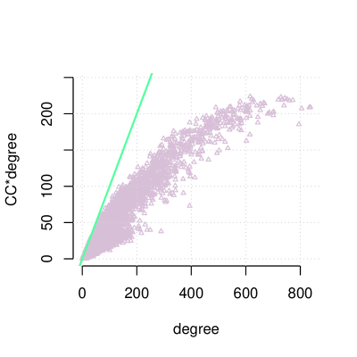
Figure S6: Plot of $\gamma_{m}d_{m}$ versus $d_{m}$ for the Luminal A group.

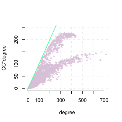
Figure S7: Plot of $\gamma_{m}d_{m}$ versus $d_{m}$ for the Luminal B group.

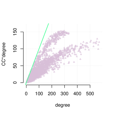
Figure S8: Plot of $\gamma_{m}d_{m}$ versus $d_{m}$ for the Basal group.

Table S1: Pathways characterizing the normal group.

Pathway Name Pathway Size Cluster Index P-value Genes Endocytosis 181 35 0.001379 HLA-B, HLA-C, HLA-E, HLA-F, HLA-G Lysosome 109 20 0.007482 CTSB, CTSL, MAN2B1, LGMN Primary immunodeficiency 34 4 6.69E-08 ADA, BTK, CD3D, CD4, CD8A, CD40, IL2RG, LCK, PTPRC 14 1.81E-06 CD8B, CD79A, IL7R, ZAP70, ICOS T cell receptor signaling pathway 103 4 1.34E-06 CD3D, CD4, CD8A, CD28, FYN, ITK, LCK, LCP2, PIK3CD, PTPN6, PTPRC, VAV1 14 0.000249 CD247, CD8B, IFNG, ZAP70, ICOS Graft-versus-host disease 36 4 9.07E-08 CD28, CD86, HLA-A, HLA-DMA, HLA-DMB, HLA-DPA1, HLA-DPB1, HLA-DRA, HLA-DRB1 14 0.001665 IFNG, KLRD1, PRF1 Natural killer cell mediated cytotoxicity 119 4 3.20E-08 CD48, FCER1G, FYN, HLA-A, ITGAL, ITGB2, LCK, LCP2, SH2D1A, PIK3CD, PRKCB, PTPN6, RAC2, TYROBP, VAV1 14 0.000336 CD247, IFNG, KLRD1, PRF1, ZAP70 35 0.002522 HLA-B, HLA-C, HLA-E, HLA-G Antigen processing and presentation 69 35 1.61E-09 B2M, HLA-B, HLA-C, HLA-E, HLA-F, HLA-G, PSME2, TAP1 4 1.80E-07 CD4, CD8A, CD74, CTSS, HLA-A, HLA-DMA, HLA-DMB, HLA-DPA1, HLA-DPB1, HLA-DRA, HLA-DRB1 20 0.001641 CTSB, CTSL, LGMN, IFI30 14 0.007611 CD8B, IFNG, KLRD1 Phagosome 138 4 4.67E-06 CTSS, FCGR2B, HLA-A, HLA-DMA, HLA-DMB, HLA-DPA1, HLA-DPB1, HLA-DRA, HLA-DRB1, ITGB2, NCF4, CORO1A, CLEC7A 35 3.40E-05 HLA-B, HLA-C, HLA-E, HLA-F, HLA-G, TAP1 20 0.000366 ATP6V1B2, CTSL, FCGR2A, FCGR3B, MSR1, NCF2 11 0.003818 C1R, COMP, ITGA5, ITGAV, THBS2, MRC2 • Uniquely enriched pathways (endocytosis and lysosome) and enriched in a larger number of clusters in the normal group than other subtypes (phagosome, antigen processing and presentation, natural killer cell mediated cytotoxicity, graft-versus-host disease, T cell receptor signaling pathway, and primary immunodeficiency). All identified clusters are indexed by their size. The cluster index indicates the order of the clusters. Note that a pathway can be enriched in multiple clusters as we performed the enrichment analysis for each cluster. P-values are adjusted to control the false discovery rate using Benjamini and Hochberg [37].

References

- Stuart et al. [2003] Joshua M Stuart, Eran Segal, Daphne Koller, and Stuart K Kim. A gene-coexpression network for global discovery of conserved genetic modules. science, 302(5643):249–255, 2003.
- Zhang and Horvath [2005] Bin Zhang and Steve Horvath. A general framework for weighted gene co-expression network analysis. Statistical applications in genetics and molecular biology, 4(1), 2005.
- Eisen et al. [1998] Michael B Eisen, Paul T Spellman, Patrick O Brown, and David Botstein. Cluster analysis and display of genome-wide expression patterns. Proceedings of the National Academy of Sciences, 95(25):14863–14868, 1998.
- Taylor et al. [2009] Ian W Taylor, Rune Linding, David Warde-Farley, Yongmei Liu, Catia Pesquita, Daniel Faria, Shelley Bull, Tony Pawson, Quaid Morris, and Jeffrey L Wrana. Dynamic modularity in protein interaction networks predicts breast cancer outcome. Nature biotechnology, 27(2):199–204, 2009.
- Barabási et al. [2011] Albert-László Barabási, Natali Gulbahce, and Joseph Loscalzo. Network medicine: a network-based approach to human disease. Nature Reviews Genetics, 12(1):56–68, 2011.
- Ravasz et al. [2002] Erzsébet Ravasz, Anna Lisa Somera, Dale A Mongru, Zoltán N Oltvai, and A-L Barabási. Hierarchical organization of modularity in metabolic networks. science, 297(5586):1551–1555, 2002.
- Wuchty et al. [2003] Stephan Wuchty, Zoltán N Oltvai, and Albert-László Barabási. Evolutionary conservation of motif constituents in the yeast protein interaction network. Nature genetics, 35(2):176–179, 2003.
- Tong et al. [2004] Amy Hin Yan Tong, Guillaume Lesage, Gary D Bader, Huiming Ding, Hong Xu, Xiaofeng Xin, James Young, Gabriel F Berriz, Renee L Brost, Michael Chang, et al. Global mapping of the yeast genetic interaction network. science, 303(5659):808–813, 2004.
- Newman [2001] Mark EJ Newman. Scientific collaboration networks. ii. shortest paths, weighted networks, and centrality. Physical review E, 64(1):016132, 2001.
- Amaral et al. [2000] Luıs A Nunes Amaral, Antonio Scala, Marc Barthelemy, and H Eugene Stanley. Classes of small-world networks. Proceedings of the national academy of sciences, 97(21):11149–11152, 2000.
- Jeong et al. [2001] Hawoong Jeong, Sean P Mason, A-L Barabási, and Zoltan N Oltvai. Lethality and centrality in protein networks. Nature, 411(6833):41–42, 2001.
- Zhang et al. [2011] Liqing Zhang, Layne T Watson, and Lenwood S Heath. A network of scop hidden markov models and its analysis. BMC bioinformatics, 12(1):191, 2011.
- Chu et al. [2012] Liang-Hui Chu, Corban G Rivera, Aleksander S Popel, and Joel S Bader. Constructing the angiome: a global angiogenesis protein interaction network. Physiological genomics, 44(19):915–924, 2012.
- Smith [2006] Reginald D Smith. The network of collaboration among rappers and its community structure. Journal of Statistical Mechanics: Theory and Experiment, 2006(02):P02006, 2006.
- Radrich et al. [2010] Karin Radrich, Yoshimasa Tsuruoka, Paul Dobson, Albert Gevorgyan, Neil Swainston, Gino Baart, and Jean-Marc Schwartz. Integration of metabolic databases for the reconstruction of genome-scale metabolic networks. BMC systems biology, 4(1):114, 2010.
- Schott [2007] James R Schott. A test for the equality of covariance matrices when the dimension is large relative to the sample sizes. Computational Statistics & Data Analysis, 51(12):6535–6542, 2007.
- Li et al. [2012] Jun Li, Song Xi Chen, et al. Two sample tests for high-dimensional covariance matrices. The Annals of Statistics, 40(2):908–940, 2012.
- Cai et al. [2013] Tony Cai, Weidong Liu, and Yin Xia. Two-sample covariance matrix testing and support recovery in high-dimensional and sparse settings. Journal of the American Statistical Association, 108(501):265–277, 2013.
- Cai and Liu [2016] T Tony Cai and Weidong Liu. Large-scale multiple testing of correlations. Journal of the American Statistical Association, 111(513):229–240, 2016.
- Zhu et al. [2017] Lingxue Zhu, Jing Lei, Bernie Devlin, and Kathryn Roeder. Testing high-dimensional covariance matrices, with application to detecting schizophrenia risk genes. The Annals of Applied Statistics, 11(3):1810, 2017.
- Subramanian et al. [2005] Aravind Subramanian, Pablo Tamayo, Vamsi K Mootha, Sayan Mukherjee, Benjamin L Ebert, Michael A Gillette, Amanda Paulovich, Scott L Pomeroy, Todd R Golub, Eric S Lander, et al. Gene set enrichment analysis: a knowledge-based approach for interpreting genome-wide expression profiles. Proc Natl Acad Sci, 102(43):15545–15550, 2005.
- Mootha et al. [2003] Vamsi K Mootha, Cecilia M Lindgren, Karl-Fredrik Eriksson, Aravind Subramanian, Smita Sihag, Joseph Lehar, Pere Puigserver, Emma Carlsson, Martin Ridderstråle, Esa Laurila, et al. Pgc-1-responsive genes involved in oxidative phosphorylation are coordinately downregulated in human diabetes. Nature genetics, 34(3):267–273, 2003.
- Consortium et al. [2004] Gene Ontology Consortium et al. The gene ontology (go) database and informatics resource. Nucleic acids research, 32(suppl 1):D258–D261, 2004.
- Kanehisa and Goto [2000] Minoru Kanehisa and Susumu Goto. Kegg: kyoto encyclopedia of genes and genomes. Nucleic acids research, 28(1):27–30, 2000.
- Khatri et al. [2012] Purvesh Khatri, Marina Sirota, and Atul J Butte. Ten years of pathway analysis: current approaches and outstanding challenges. PLoS computational biology, 8(2):e1002375, 2012.
- Meinshausen and Bühlmann [2006] Nicolai Meinshausen and Peter Bühlmann. High-dimensional graphs and variable selection with the lasso. The Annals of Statistics, pages 1436–1462, 2006.
- Friedman et al. [2008] Jerome Friedman, Trevor Hastie, and Robert Tibshirani. Sparse inverse covariance estimation with the graphical lasso. Biostatistics, 9(3):432–441, 2008.
- Yuan and Lin [2007] Ming Yuan and Yi Lin. Model selection and estimation in the gaussian graphical model. Biometrika, 94(1):19–35, 2007.
- Banerjee et al. [2008] Onureena Banerjee, Laurent El Ghaoui, and Alexandre d’Aspremont. Model selection through sparse maximum likelihood estimation for multivariate gaussian or binary data. Journal of Machine learning research, 9(Mar):485–516, 2008.
- Rothman et al. [2008] Adam J Rothman, Peter J Bickel, Elizaveta Levina, Ji Zhu, et al. Sparse permutation invariant covariance estimation. Electronic Journal of Statistics, 2:494–515, 2008.
- Levina et al. [2008] Elizaveta Levina, Adam Rothman, and Ji Zhu. Sparse estimation of large covariance matrices via a nested lasso penalty. The Annals of Applied Statistics, pages 245–263, 2008.
- NCI and NHGRI [2018] NCI and NHGRI. The cancer genome atlas, 2018. URL https://cancergenome.nih.gov. National Cancer Institute and National Human Genome Research Institute, The Cancer Genome Atlas.
- Frankl and Maehara [1990] Peter Frankl and Hiroshi Maehara. Some geometric applications of the beta distribution. Annals of the Institute of Statistical Mathematics, 42:463–474, 1990.
- Yeung et al. [2002] MK Stephen Yeung, Jesper Tegnér, and James J Collins. Reverse engineering gene networks using singular value decomposition and robust regression. Proceedings of the National Academy of Sciences, 99(9):6163–6168, 2002.
- Bar and Schifano [2019] Haim Bar and Elizabeth D. Schifano. Differential variation and expression analysis. Stat, 8(1):e237, 2019. doi: 10.1002/sta4.237. URL https://onlinelibrary.wiley.com/doi/abs/10.1002/sta4.237.
- Dempster et al. [1977] A. P. Dempster, N. M. Laird, and D. B. Rubin. Maximum likelihood from incomplete data via the EM algorithm. Journal of the Royal Statistical Society, Series B, 39(1):1–38, 1977.
- Benjamini and Hochberg [1995] Yoav Benjamini and Yosef Hochberg. Controlling the false dicovery rate-a practical and powerful approach to multiple testing. Journal of the Royal Statistical Society Series B, 57(3):499–517, 1995.
- Zhao et al. [2015] Tuo Zhao, Xingguo Li, Han Liu, Kathryn Roeder, John Lafferty, and Larry Wasserman. huge: High-Dimensional Undirected Graph Estimation, 2015. URL https://CRAN.R-project.org/package=huge. R package version 1.2.7.
- Barabási and Albert [1999] Albert-László Barabási and Réka Albert. Emergence of scaling in random networks. Science, 286(5439):509–512, 1999.
- Allahyar et al. [2019] Amin Allahyar, Joske Ubels, and Jeroen de Ridder. A data-driven interactome of synergistic genes improves network-based cancer outcome prediction. PLOS Computational Biology, 15(2):1–21, 02 2019. doi: 10.1371/journal.pcbi.1006657. URL https://doi.org/10.1371/journal.pcbi.1006657.
- Staiger et al. [2013] Christine Staiger, Sidney Cadot, Balázs Györffy, Lodewyk Wessels, and Gunnar Klau. Current composite-feature classification methods do not outperform simple single-genes classifiers in breast cancer prognosis. Frontiers in Genetics, 4:289, 2013. ISSN 1664-8021. doi: 10.3389/fgene.2013.00289. URL https://www.frontiersin.org/article/10.3389/fgene.2013.00289.
- Towles et al. [2016] Joanna K Towles, Rebecca N Clark, Michelle D Wahlin, Vinita Uttamsingh, Allan E Rettie, and Klarissa D Jackson. Cytochrome p450 3a4 and cyp3a5-catalyzed bioactivation of lapatinib. Drug Metabolism and Disposition, 44(10):1584–1597, 2016.
- Huszno et al. [2015] Joanna Huszno, Agnieszka Badora, and Elżbieta Nowara. The influence of steroid receptor status on the cardiotoxicity risk in her2-positive breast cancer patients receiving trastuzumab. Archives of medical science: AMS, 11(2):371, 2015.
- Fisher et al. [2010] Robert D Fisher, Mark Ultsch, Andreas Lingel, Gabriele Schaefer, Lily Shao, Sara Birtalan, Sachdev S Sidhu, and Charles Eigenbrot. Structure of the complex between her2 and an antibody paratope formed by side chains from tryptophan and serine. Journal of molecular biology, 402(1):217–229, 2010.
- Miolo et al. [2016] Gianmaria Miolo, Elena Muraro, Donatella Caruso, Diana Crivellari, Anthony Ash, Simona Scalone, Davide Lombardi, Flavio Rizzolio, Antonio Giordano, and Giuseppe Corona. Pharmacometabolomics study identifies circulating spermidine and tryptophan as potential biomarkers associated with the complete pathological response to trastuzumab-paclitaxel neoadjuvant therapy in her-2 positive breast cancer. Oncotarget, 7(26):39809, 2016.
- Cook et al. [2011] Katherine L Cook, Ayesha N Shajahan, and Robert Clarke. Autophagy and endocrine resistance in breast cancer. Expert review of anticancer therapy, 11(8):1283–1294, 2011.
- Anurag et al. [2018] Meenakshi Anurag, Nindo Punturi, Jeremy Hoog, Matthew N Bainbridge, Matthew J Ellis, and Svasti Haricharan. Comprehensive profiling of dna repair defects in breast cancer identifies a novel class of endocrine therapy resistance drivers. Clinical Cancer Research, 24(19):4887–4899, 2018.