“Divide-and-Conquer” Semiclassical Molecular Dynamics: An Application to Water Clusters

Abstract

We present an investigation of vibrational features in water clusters performed by means of our recently established divide-and-conquer semiclassical approach (M. Ceotto, G. Di Liberto, R. Conte Phys. Rev. Lett. 119, 010401 (2017)). This technique allows to simulate quantum vibrational spectra of high dimensional systems starting from full-dimensional classical trajectories and projection of the semiclassical propagator onto a set of lower dimensional subspaces. The potential energy surface employed is a many-body representation up to three-body terms, in which monomers and two-body interactions are described by the high level WHBB water potential, while, for three-body interactions, calculations adopt a fast permutationally-invariant ab initio surface at the same level of theory of the WHBB 3-body potential. Applications range from the water dimer up to the water decamer, a system made of 84 vibrational degrees of freedom. Results are generally in agreement with previous variational estimates in the literature. This is particularly true for the bending and the high-frequency stretching motions, while estimates of modes strongly influenced by hydrogen bonding are red shifted, in a few instances even substantially, as a consequence of the dynamical and global picture provided by the semiclassical approach.

I Introduction

The water molecule has often attracted the attention of the scientific community due to the fundamental role it plays for life on our planet.¹; ²; ³; ⁴; ⁵; ⁶; ⁷ In chemical and physical processes involving water, hydrogen bonding is crucial⁸; ⁹ allowing the formation of supra-molecular structures (made of several water molecules) known as water clusters.¹⁰; ¹¹; ¹² Water clusters are major players in atmospheric photocatalytic processes,¹³; ¹⁴ and they have been largely investigated by both theoretical and experimental approaches focused on their structure and interaction network. Many studies have been also devoted to protonated water clusters, which represent suitable and realistic models for understanding the proton transfer mechanism in aqueous solutions.¹⁵ Furthermore, the interest in water clusters and systems where one or more water molecules interact with other species has recently involved methane and hydrogen clathrates,¹⁶; ¹⁷; ¹⁸ HCl hydrates,¹⁹; ²⁰; ²¹ or even solvated ions.²²; ²³; ²⁴; ²⁵

Focusing on homogeneous water clusters, experimental investigations involving systems of different size ranging from the dimer up to the decamer have shown that the vibrational spectral features of the OH bonds are extremely sensitive to hydrogen interactions and dependent on the specific cluster network,²⁶; ²⁷; ²⁸ while deuteration studies have demonstrated that the OH vibrational frequencies may serve as a probe for hydrogen bonding.²⁹ Experimental findings also include the evidence that the OH stretches involved in the hydrogen bonds undergo a red shift sometimes as large as 600-700 cm^-1,³⁰; ³¹ while the frequency of vibration of the free OH stretches is almost unchanged and the bending region characterized by a slight but progressive blue shift with increasing cluster size.³² The main vibrational features of these clusters are distributed in the 1500-4000 cm^-1 region. The lowest in frequency (at about 1600 cm^-1) can be assigned to the bending motion,³³ while the other features are associated to the OH stretch and situated at around 3000, 3500, and 3700 cm^-1.³⁴

From a theoretical point of view, important and pioneering work has been performed by Xantheas and co-workers, who revealed that the potential energy surface (PES) of even small clusters is very complicated because of the many minima that can be located on it. They also showed that for properly studying these systems a high level of electronic structure theory must be employed, and that the zero-point-energy correction is definitely not negligible to determine the relative stability between the several minima.³⁵ Energy differences among these minima are often smaller than a fraction of kcal/mol, so an investigation based exclusively on the global minimum is probably not accurate enough to properly account for the overall properties.³⁶; ³⁷; ³⁸; ³⁹; ⁴⁰; ⁴¹

The complexity of the water cluster PESs makes their construction difficult, while the high level of electronic theory required rules out the possibility to resort to on-the-fly ab initio approaches. However, the development in the past years of precise fitting procedures has opened up the way to many theoretical investigations of variously-sized water clusters.⁴²; ⁴³; ⁴⁴; ⁴⁵; ⁴⁶; ⁴⁷; ⁴⁸; ⁴⁹; ⁵⁰ Among them we recall the work done by Partridge and Schwenke⁵¹ in which they developed an accurate one body potential, the parametrization of the water model by Burnham and Leslie,⁵² or, more recently, the effort profused by the groups of Xantheas and Bowman which led to more and more accurate water potentials.⁵³; ⁵⁴; ⁵⁵; ⁵⁶; ⁵⁷; ⁵⁸; ⁵⁹; ⁶⁰

A practical way to describe the PES of a water cluster is through a many-body representation. Several studies, including those by Xantheas, Clary, Paesani and their co-workers to name a few remarkable ones, demonstrated that the representation can be truncated to the three-body terms without significant loss of accuracy.⁶¹; ⁶²; ⁴⁸ In particular, Bowman’s HBB,⁵⁵ WHBB,⁶³; ⁶⁰ and WHBB2 PESs⁶⁰ include terms up to the three-body interaction and were shown to be very accurate and flexible for water clusters of any size, thus permitting state-of-art VCI calculations for the vibrational frequencies.⁵⁸ These calculations were based on the local monomer approach which permits to accurately simulate spectra and to deal with even large water clusters which otherwise would not be computationally affordable.

We deem that an alternative, quantum dynamical theoretical approach for spectroscopy calculations of water clusters could more realistically describe the hydrogen bonding among water monomers and better uncover possible resonances between overtones and fundamental vibrations. The latter may for instance involve the OH bending overtones and the OH stretching fundamental vibrations, which occur at nearby frequency values. Such a quantum dynamical approach can be provided by the semiclassical theory (SC) in its initial value representation version (SCIVR). SCIVR builds a bridge between classical and quantum physics, since it allows to approximate the quantum propagator reliably by using only dynamical quantities that are generated from a classical simulation.⁶⁴; ⁶⁵; ⁶⁶; ⁶⁷; ⁶⁸; ⁶⁹; ⁷⁰; ⁷¹; ⁷²; ⁷³; ⁷⁴; ⁷⁵; ⁷⁶ Specifically, the time averaged version of the quantum propagator is able to detect quantum effects on small- and medium-sized molecules accurately.⁷⁷; ⁷⁸; ⁷⁹; ⁸⁰; ⁸¹; ⁸²; ⁸³; ⁸⁴; ⁸⁵; ⁸⁶; ⁸⁷; ⁸⁸; ⁸⁹; ⁹⁰ Recently, we have proposed a method called Divide-and-Conquer Semiclassical Initial Value Representation (DC SCIVR)⁹¹; ⁹² which makes semiclassical dynamics viable also for large molecules. In DC SCIVR the full-dimensional problem is divided into a set of lower dimensional ones before proceeding with a proper set of SC calculations constrained within the low-dimensional subspaces but still based on the full-dimensional classical trajectory.

In this work we present a theoretical investigation of variously sized water clusters by means of our recently established DC SCIVR. Results show that quantum anharmonic effects are not negligible and dynamical effects associated to the strong hydrogen-bond interactions are relevant. We also illustrate a methodology for selecting a few relevant minima in order to run semiclassical simulations with very reduced computational costs yet retaining good accuracy. In the next Section we describe the computational approach employed. Then we report our results starting from the investigation of the vibrational features of the smallest water clusters: the dimer and the trimer. Finally the focus shifts to the water hexamer prism, for which we present some evidences of the important role of hydrogen bond interactions, and to the water decamer, whose vibrational features we are able to precisely describe by employing just a few selected trajectories. The paper ends with a brief summary and the presentation of our conclusions.

II Computational Methods

The global PES employed in the calculations has been constructed according to the many-body representation (truncated at the three-body level) reported in Eq. (1)

$$V({\bf q})=\sum_{i}^{N}V^{W}({\bf q}_{i})+\sum_{j>i}^{N}V^{W-W}({\bf q}_{i},{\bf q}_{j})+\sum_{k>j>i}^{N}V^{W-W-W}({\bf q}_{i},{\bf q}_{j},{\bf q}_{k}),$$ (1)

where the $W$ superscripts stand for “water”, $N$ indicates the number of water monomers in the cluster, ${\bf q}$ represents the collection of all atomic coordinates, while ${\bf q}_{i}$ is the set of coordinates corresponding to atoms exclusively belonging to the i-th water monomer. Specifically, we used the Partridge-Schwenke potential for the 1-body ($W$) term;⁵¹ the 2-body ($W-W$) interaction surface has been extracted from the highly accurate WHBB potential;⁵⁹ a new, computationally-efficient potential was built for the 3-body ($W-W-W)$ interaction starting from the same database of about 40,000 ab initio points used for the WHBB 3-body potential but employing a previously developed fitting procedure for many-body interaction potentials.¹⁶; ⁹³; ¹⁷; ⁹⁴; ⁹⁵; ⁹⁶ This new 3-body potential is based on 1,181 polynomials, it has an rms of 46 cm^-1 calculated with respect to the database of ab initio points (51 cm^-1 for WHBB with maximum polynomial order 5), and it is about 70 times faster than the 3-body potential (maximum polynomial order 5) included in the WHBB suite. A $W-W-W$ potential very similar in speed to the one employed here has been recently and independently developed by Bowman and coworkers and included in a new version of their water potential, named WHBB2.⁶⁰

Vibrational frequencies have been determined upon calculation of semiclassical power spectra. Semiclassical approaches aim at regaining quantum information starting from classically-evolved trajectories and their mathematical formalism is obtained by approximating Feynman’s quantum propagator. Feynman’s path integral formulation⁹⁷ is a renowned way to represent the quantum propagator in which the probability of going from an initial state $\mathbf{q}_{0}$ to a final one $\mathbf{q}_{t}$ can be obtained by summing up over all the paths that connect the two states. A weight that depends on its action is associated to each path

$$\left\langle\mathbf{q}_{t}\left|e^{-i\hat{H}t/\hbar}\right|\mathbf{q}_{0}\right\rangle \int_{\mathbf{q}_{0}}^{\mathbf{q}_{t}}\mathcal{D}\left[\mathbf{q}\left(t\right)\right]e^{iS_{t}\left[\mathbf{q}_{0},\mathbf{q}_{t}\right]/\hbar}$$= (2)

Upon stationary-phase approximation, the integral in Eq. (2) becomes a sum over the paths that give the major contribution. Such paths are the classical ones and the approximation is exact up to quadratic potentials.⁹⁸ The result coincides with the van Vleck version of the semiclassical propagator,⁹⁹ which is reported in Eq. 3.

$$\left\langle\mathbf{q}_{t}\left|e^{-i\hat{H}t/\hbar}\right|\mathbf{q}_{0}\right\rangle\approx\sum_{\text{cl. paths}}\sqrt{\frac{1}{\left(2\pi i\hbar\right)^{F}}\left|-\frac{\partial^{2}S_{t}^{cl}\left(\mathbf{q}_{0},\mathbf{q}_{t}\right)}{\partial\mathbf{q}_{t}\partial\mathbf{q}_{0}}\right|}e^{iS_{t}^{cl}\left(\mathbf{q}_{0},\mathbf{q}_{t}\right)/\hbar-i\nu\pi/2}$$

$$=\text{$\sum_{\text{cl. paths}}\sqrt{\frac{1}{\left(2\pi i\hbar\right)^{F}}\left|\frac{\partial\mathbf{q}_{t}}{\partial\mathbf{p}_{0}}\right|^{-1}}e^{iS_{t}^{cl}\left(\mathbf{q}_{0},\mathbf{q}_{t}\right)/\hbar-i\nu\pi/2}$},$$ (3)

where $F$ is the number of degrees of freedom, $\mathbf{p}_{0}$ is the initial momentum of the classical path, and $\upsilon$ is the Maslov index, which ensures the continuity of the complex square root. A more user-friendly version of the SC propagator has been worked out by Miller, who introduced the Initial Value Representation (IVR)¹⁰⁰ of the van Vleck propagator. Application of this SCIVR propagator to the survival amplitude of a generic reference wavefunction $\left|\chi\right\rangle$ leads to

$$\left\langle\chi\left|e^{-i\hat{H}t/\hbar}\right|\chi\right\rangle\approx\int\int \mathbf{p}_{0} \mathbf{q}_{0}\sqrt{\frac{1}{\left(2\pi i\hbar\right)^{F}}\left|\frac{\partial\mathbf{q}_{t}}{\partial\mathbf{p}_{0}}\right|}\chi^{*}\left(\mathbf{q}_{t}\right)\chi\left(\mathbf{q}_{0}\right)e^{iS_{t}^{cl}\left(\mathbf{p}_{0},\mathbf{q}_{0}\right)/\hbar-i\nu\pi/2}$$dd (4)

Eq. (4) points out the two main advantages of an IVR approach, i.e. the difficult quest for a solution to a double-boundary problem is substituted by the easy generation of the classical trajectory starting from its initial phase-space conditions ($\mathbf{p}_{0},\mathbf{q}_{0}$), plus the removal of the partial derivative at the denominator of Eq. (3) which may lead to an unphysical divergence of the propagator. Another milestone contribution to SC dynamics came from Heller with the introduction of the coherent state representation. Coherent states are suitable to describe bound as well as unbound systems since their projection onto the coordinate space consists in a Gaussian-shaped real part and a free-particle imaginary part as follows¹⁰¹; ¹⁰²

$$\left\langle\mathbf{x}\left|\mathbf{p}_{t}\mathbf{q}_{t}\right.\right\rangle \left(\frac{det(\Gamma)}{\pi^{F}}\right)^{\frac{1}{4}}e^{-\frac{1}{2}\left(\mathbf{x}-\mathbf{q}_{t}\right)^{T}\Gamma\left(\mathbf{x}-\mathbf{q}_{t}\right)+\frac{i}{\hbar}\mathbf{p}_{t}^{T}\left(\mathbf{x}-\mathbf{q}_{t}\right)}$$= (5)

The width of the multidimensional coherent state is generally chosen to be a diagonal matrix ($\Gamma$). In the case of vibrational studies the width matrix can be built by setting its diagonal elements equal to the square roots of the eigenvalues of the Hessian matrix at the equilibrium geometry, i.e. the harmonic frequencies. The semiclassical propagator in the coherent state representation is the Herman Kluk (HK) propagator¹⁰³

$$\left\langle\chi\left|e^{-i\hat{H}t/\hbar}\right|\chi\right\rangle\approx\left(\frac{1}{2\pi\hbar}\right)^{F}\iintop \mathbf{p}_{0} \mathbf{q}_{0}C_{t}\left(\mathbf{p}_{0},\mathbf{q}_{0}\right)e^{\frac{i}{\hbar}S_{t}\left(\mathbf{p}_{0},\mathbf{q}_{0}\right)}\left\langle\chi\right.\left|\mathbf{p}_{t}\mathbf{q}_{t}\left\rangle\right\langle\mathbf{p}_{0}\mathbf{q}_{0}\right|\left.\chi\right\rangle$$dd, (6)

where the pre-exponential factor - $C_{t}\left(\mathbf{p}_{0},\mathbf{q}_{0}\right)$ - accounts for quantum effects but is affected by the possible chaotic behavior of the classical trajectories initiated from the phase space points $\left(\mathbf{p}_{0},\mathbf{q}_{0}\right)$.

$$\text{$C_{t}\left(\mathbf{p}_{0},\mathbf{q}_{0}\right)$=$\sqrt{\mbox{det}\left[\frac{1}{2}\left(\mathbf{M_{qq}}+{\bf\Gamma}^{-1}\mathbf{M_{pp}}\mathbf{\Gamma}+\frac{i}{\hbar{\bf\Gamma}}\mathbf{M_{pq}}-i\mathbf{\hbar{\bf\Gamma}M_{qp}}\right)\right]}$},$$ (7)

where ${\bf M_{ij}}=\partial{\bf i}_{t}/\partial{\bf j}_{0}\quad{\bf i},{\bf j}={\bf p},{\bf q}$ is itself a matrix which represents a generic element of the monodromy matrix.⁹⁸; ¹⁰⁴

The power spectrum of the Hamiltonian $\hat{H}$ is the Fourier transform of Eq. (6), i.e.

I$$\left(E\right) \left(\frac{1}{2\pi\hbar}\right)^{F+1}\int_{-\infty}^{+\infty} e^{iEt/\hbar}\iintop \mathbf{p}_{0} \mathbf{q}_{0}C_{t}\left(\mathbf{p}_{0},\mathbf{q}_{0}\right)e^{\frac{i}{\hbar}S_{t}\left(\mathbf{p}_{0},\mathbf{q}_{0}\right)}\left\langle\chi\right.\left|\mathbf{p}_{t}\mathbf{q}_{t}\left\rangle\right\langle\mathbf{p}_{0}\mathbf{q}_{0}\right|\left.\chi\right\rangle$$=dt dd. (8)

Unfortunately the standard formulation of the HK propagator is difficult to converge and computationally very demanding.¹⁰⁵; ¹⁰⁶ To overcome this issue, Kaledin and Miller demonstrated that it is possible to time-average (TA) Eq. (6) to arrive to an expression for the spectral density I(E) - see Eq. (9) - where the phase-space integrand is positive-definite and, consequently, the integral is much easier to converge⁷⁷

I$$\left(E\right) \left(\frac{1}{2\pi\hbar}\right)^{F}\iintop \mathbf{p}_{0} \mathbf{q}_{0}\frac{1}{2\pi\hbar T}\left|\intop_{0}^{T}dte^{\frac{i}{\hbar}\left[S_{t}\left(\mathbf{p}_{0},\mathbf{q}_{0}\right)+Et+\phi\left(t\right)\right]}\left\langle\bm{\chi}\left|\mathbf{p}_{t}\mathbf{q}_{t}\right.\right\rangle\right|^{2}$$=dd. (9)

Eq (9) is very accurate for small and medium sized molecules, but, unfortunately, runs out of steam when the system dimensionality gets higher than 25-30 degrees of freedom due to the so-called curse of dimensionality. To overcome this issue we have recently developed a Divide-and-Conquer semiclassical method, which allows to obtain the overall power spectrum as a composition of partial spectra.⁹¹

In the following, we briefly recall how DC SCIVR works. The basic idea is to compute a set of power spectra by operating in lower-dimensional subspaces but keeping the dynamics full-dimensional. Among the approaches we have recently illustrated for an effective grouping of the modes into different subspaces,⁹² in this work we have adopted the so-called Hessian approach, which consists in averaging the Hessian off-diagonal elements $\tilde{H}_{ij}$ along a preliminary trajectory with harmonic zero-point energy and in comparing them to a threshold value $\varepsilon$. If the vibrational modes i and j satisfy the condition $\tilde{H}_{ij}\geq\varepsilon$, they are enrolled in the same subspace. Also, they belong to the same subspace if a third mode k exists such that the conditions $\tilde{H}_{ik}\geq\varepsilon$ and $\tilde{H}_{kj}\geq\varepsilon$ are both satisfied. Eq. (9) consequently changes to

$$\widetilde{I}\left(E\right) \left(\frac{1}{2\pi\hbar}\right)^{M}\iintop \tilde{\mathbf{p}}\left(0\right) \tilde{\mathbf{q}}\left(0\right)\frac{1}{2\pi\hbar T}\left|\intop_{0}^{T}e^{\frac{i}{\hbar}\left[\tilde{S}_{t}\left(\tilde{\mathbf{p}}\left(0\right),\tilde{\mathbf{q}}\left(0\right)\right)+Et+\tilde{\phi}_{t}\right]}\left\langle\tilde{\bm{\chi}}\left|\tilde{\mathbf{p}}\left(t\right)\tilde{\mathbf{q}}\left(t\right)\right.\right\rangle dt\right|^{2}$$=dd, (10)

where $\tilde{f}$ indicates the projection of the generic $f$ quantity onto an M-dimensional subspace. Matrices (Hessian and Gaussian width ones) as well as vectors (momentum and position) can be easily projected by means of Hinsen and Kneller’s singular value decomposition.¹⁰⁷; ¹⁰⁸; ⁹¹ Projection of the action is more elaborated due to the general non-separability of the potential energy. In fact, the projected action is calculated through straightforward projection of the kinetic energy, which is separable, and by means of a projected potential - see Eq. (11). In the projected potential the variables external to the M-dimensional subspace (${\bf q}_{F-M})$ are treated as parameters and a time-dependent field ($\lambda$), able to account for the non-separability of the potential and to regain the exact potential in separable instances, is introduced.⁹¹; ⁹²

$$\begin{array}[]{c}V({\bf\tilde{{\bf q}}}_{M})=V({\bf\tilde{{\bf q}}}_{M};{\bf q}_{F-M}^{eq})+\lambda(t);\\ \lambda(t)=V({\bf\tilde{{\bf q}}}_{M};{\bf q}_{F-M})-V({\bf\tilde{{\bf q}}}_{M}^{eq};{\bf q}_{F-M})-V({\bf\tilde{{\bf q}}}_{M};{\bf q}_{F-M}^{eq})\end{array}$$ (11)

For water clusters, due to the large number of low frequency modes which may make spectra very noisy, it is necessary to introduce an additional device consisting in giving no initial kinetic energy to modes different from bendings and OH stretchings. Several of these modes present very low vibrational features associated to the libration motions of frustrated translations and rotations. Below we will show that this ad-hoc approximation does not spoil the accuracy of the calculated frequencies for bendings and stretchings. Furthermore, we employed a recently developed and accurate approximation to the pre-exponential factor,⁷⁹ which has permitted to retain the chaotic trajectories that in a basic application of DC SCIVR would have been otherwise discarded. The approximation exploits the exact Log-derivative formulation of the pre-exponential factor¹⁰⁹ in which the latter depends on a matrix $\mathbf{R}_{t}$ determined by solving an appropriate Riccati equation

$$\text{\text{$C_{t}\left(\mathbf{p}_{0},\mathbf{q}_{0}\right)$=}$\sqrt{\mbox{det}\left[\frac{1}{2}\left(I+\frac{i}{\hbar{\bf\Gamma}}\mathbf{R}_{t}\right)\right]}e^{\frac{1}{2}\intop_{0}^{t}d\tau\text{Tr}\left[\mathbf{R}_{\tau}\right]}$},$$ (12)

where $\mathbf{R}_{t}$ can be approximated as

$$\mathbf{R}_{t} \frac{i}{2}\left[\frac{\mathbf{K}_{t}}{\hbar\bm{\Gamma}}+\hbar\bm{\Gamma}\right] \frac{i}{4}\frac{\left(\hbar\bm{\Gamma}-\frac{\mathbf{K}_{t}}{\hbar\bm{\Gamma}}\right)^{2}}{\left(\hbar\bm{\Gamma}+\frac{\mathbf{K}_{t}}{\hbar\bm{\Gamma}}\right)}$$=-+, (13)

and $\mathbf{K}_{t}$ is the Hessian matrix.

According to the convergence pattern of TA-SCIVR, the power spectra would require generation of a number of trajectories of the order of a thousand per degree of freedom to reach convergence. A reliable procedure to alleviate computational overheads is needed for application of DC SCIVR to large molecular systems. For this purpose, we implemented the Multiple Coherent State (MC) approach into DC-SCIVR by running one trajectory per each of the $N_{st}$ coherent states that make up the reference state $|\chi\rangle$ according to Eq. (14).

$$|\chi\rangle=\sum_{k=1}^{N_{st}}\prod_{j=1}^{M}\text{$\left|p_{eq,j}^{(k)}q_{eq,j}^{(k)}\right\rangle$+$\xi_{j}^{(k)}\left|-p_{eq,j}^{(k)}q_{eq,j}^{(k)}\right\rangle$},$$ (14)

where $\xi_{j}^{(k)}$ is a parameter that allows to distinguish between different vibrational signals according to their symmetry or parity. In this way, as demonstrated in the literature,⁸³; ⁸¹; ⁸⁰; ¹¹⁰ accurate spectra can be recovered by running just a few or even a single classical trajectory provided it is close in energy to the actual quantum vibrational frequency. To get more information than a traditional discrete Fourier transform, the time integration of Eq.(10) is performed using the compress sensing signal processing technique.¹¹¹

The divide-and-conquer approach can be also implemented to calculate classical-like spectral densities from the Fourier transform of the velocity-velocity correlation function

$$I\left(E\right)=\int dte^{iEt}\biggl{\langle}\mathbf{v}\left(t\right)\mathbf{v}\left(0\right)\biggr{\rangle}=\int_{-\infty}^{+\infty}dte^{iEt}\int d\mathbf{q}_{0}d\mathbf{p}_{0}\rho\left(\mathbf{q}_{0},\mathbf{p}_{0}\right)\mathbf{v}\left(t\right)\mathbf{v}\left(0\right)$$ (15)

By adding a further integration ($\frac{1}{T}\int_{0}^{T}dt$) we can derive the time-averaged version of Eq. (15), similarly to what Miller and co-workers have obtained for semiclassical spectral densities,⁷⁷; ⁷⁸ and Kaledin and Bowman for classical simulations ¹¹²

$$I\left(E\right)=lim_{T\rightarrow+\infty}\int d\mathbf{q}_{0}d\mathbf{p}_{0}\rho\left(\mathbf{p}_{0},\mathbf{q}_{0}\right)\frac{1}{2T}\Biggl{|}\int_{0}^{T}dte^{iE\left(t\right)}\mathbf{v}\left(t\right)\Biggr{|}^{2}.$$ (16)

Reduced dimensional spectra can be calculated by means of the projected classical quantities obtained with the same procedure employed in DCSCIVR.⁹¹; ⁹² The final working formula is

$$I\left(E\right)=lim_{T\rightarrow+\infty}\int d\mathbf{\tilde{q}}_{0}d\mathbf{\tilde{p}}_{0}\tilde{\rho}\left(\tilde{\mathbf{q}}_{0},\mathbf{\tilde{p}}_{0}\right)\frac{1}{2T}\Biggl{|}\int_{0}^{T}dte^{iE\left(t\right)}\mathbf{\tilde{v}}\left(t\right)\Biggr{|}^{2},$$ (17)

where $\tilde{\rho}({\bf p}_{0},{\bf q}_{0})$ is the sampling phase-space distribution function in reduced dimensionality.

III Results and Discussion

We start off by demonstrating the reliability of our DC-SCIVR calculations of small water clusters such as the dimer and trimer, for which accurate MultiMode and experimental energy levels are available. Then, we move to the water hexamer showing the influence of dynamical effects on spectral densities. Finally, as an application to a larger system, we calculate the vibrational energy levels of the water decamer.

III.1 Water Dimer (H₂O)₂

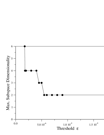
Figure 1: Dependence of the maximum subspace dimensionality on the arbitrary Hessian threshold for the water dimer.

The smallest water cluster - the dimer - has 12 vibrational degrees of freedom, two of which are bendings while other four are OH stretchings. To calculate these six relevant frequencies of vibration, we first tried to employ a 6-dimensional work subspace to collect all bendings and stretchings together but, unfortunately, it was not possible to get a well-resolved spectroscopic signal. To overcome this issue, we applied the DC-SCIVR partitioning to decrease the maximum subspace dimension down to 2 as suggested by the large plateau which can be easily identified from the analysis of the maximum subspace dimensionality vs Hessian threshold dependence shown in Figure (1).

In our calculations we employed a threshold value $\varepsilon=1.8\cdot 10^{-5}$. Table (1) presents experimental values,²⁷ MultiMode (MM) and Local Monomer Model (LMM) data,⁵⁸ and our semiclassical DC-SCIVR results based on different sets of trajectories. The outcomes of single-trajectory simulations (based on a dynamics 30,000 atomic time units long) that employed the multiple coherent procedure within the subspaces (MC-DC SCIVR) are reported in the last column of the Table. The mean absolute error (MAE) with respect to experimental values (78 cm^-1) is not satisfactory especially if compared to the MAE values of the benchmark MM and LMM calculations (25 and 23 cm^-1 respectively). To understand the reasons of such inaccuracy and try to improve results, we investigated the presence of additional minima on the surface which may be neglected in a single-trajectory simulation but, at the same time, may influence the semiclassical results. This is true if these local minima are very close in energy to the global minimum.¹¹⁰ For this purpose we explored the PES by means of damped-dynamics runs, and found 4 local minima just about 200 cm^-1 higher in energy than the global minimum. The damped dynamics was performed by sampling 1,000 trajectories according to a Husimi distribution around the global minimum. The damping parameter has been chosen according to a trade-off between the necessity of exploring large regions of the PES and the need to limit the simulation times. In practice, we decreased the kinetic energy by a factor equal to 0.99 at each step of the dynamics and checked that it was terminated in a minimum (either local or global) by looking at the sign of the eigenvalues of the Hessian matrix calculated at that geometry. Then, we re-applied the MC-DC-SCIVR approach by running 5 trajectories per subspace this time, with each trajectory starting from a different minimum and the MAE shifts from 78 to a much improved 48 cm^-1, which is not far from the accuracy obtained in other previous semiclassical calculations.⁸⁰ This outcome will be exploited in treating much larger clusters for which semiclassical calculations can be performed only if based on a small number of trajectories. The multiple-minima effect can also partially explain the difference between DC-SCIVR simulations (that visit all 5 minima) and the single-well reference MM or LMM calculations.

To check the reliability of MC-DC-SCIVR simulations we also performed standard, fully converged, DC-SCIVR simulations. Convergence has been reached by employing 10,000 trajectories, but 5,000-trajectory simulations were found to be already reliable. We started all the trajectories with the cluster in its equilibrium geometry. Initial atomic velocities were extracted, for each subspace calculation, from the chosen distribution of the normal mode initial kinetic energy. Specifically, for modes included in the subspace under investigation a Husimi distribution centered on momentum values corresponding to one quantum of harmonic excitation was employed; other bending and stretching motions belonging to different subspaces were instead assigned the corresponding harmonic zero-point energy contribution. Finally, as anticipated in the previous Section, all other low frequency modes were given no initial kinetic energy. Furthermore, harmonic frequencies served to define the coherent state and Husimi distribution widths. Each trajectory was evolved for a total of 30,000 atomic time units. Semiclassical investigations performed on trajectories twice as long provided no significant differences in the vibrational frequencies indicating that 30,000 atomic units is a long enough evolution time to achieve numerical convergence. MAE values for simulations based on 10,000 and 5,000 trajectories are equal to 32 and 39 cm^-1respectively. The MAE value obtained with MC-DC-SCIVR based on 5 tailored trajectories (48 cm^-1) is not far from those values, confirming the reliability of the computationally-cheaper approach. From the results it is evident the separation between the bending and stretching frequencies, and that MC-DC SCIVR must be adopted upon identification of all relevant minima. A final comparison to the experiment demonstrates that standard DC SCIVR is also able to detect the high frequency stretching overtones with reasonable accuracy.

Figure (2) shows the peaks obtained with MC-DC SCIVR employing 5 trajectories per subspace, and reports MultiMode and harmonic frequency estimates for a visual comparison. We observe that in our semiclassical spectra, because of the interaction between different modes, multiple-peak features appear as, for instance, in the case of mode 10 (which shows a shoulder at the frequency of mode 9), or as in the case of mode 9 and overtones of modes 7 and 8. The interaction between the bending overtones and the lower frequency stretches involved in hydrogen bondings is a general feature of water clusters which we found also in larger ones and which complicates the aspect of the simulated spectra.

Table 1: Vibrational frequencies of the water dimer, in $\text{c$m^{-1}$}.$ Assignments of mode excitations are reported in the first column; the following columns present, in order, the experimental results (Exp), the harmonic estimates (HO), Multimode (MM) and Local Monomer Model (LMM) results, DC-SCIVR frequencies obtained from 5,000 and 10,000 trajectories, MC-DC-SCIVR frequencies based on 5 trajectories, and MC-DC-SCIVR results from a single trajectory started from the global minimum. The mean absolute errors (MAE) are relative to the experimental values. ^a from Ref. 27; ^b from Ref. 58.

Index	Expa	HO	MMb	LMMb	DC SCIVR10k	DC SCIVR${}_{\text{5k}}$	MC-DC SCIVR5 trajs, multmin	MC-DC SCIVR${}_{\text{1 traj}}$
$7_{1}$	1600	1650	1588	1595	1597	1597	1562	1572
$8_{1}$	1617	1669	1603	1602	1585	1578	1588	1578
$7_{2}$	3163	3300	3144	3153	3154	3178	3128	3156
$8_{2}$	3194	3338	3157	3168	3130	3100	3180	3156
$9_{1}$	3591	3758	3573	3550	3550	3539	3526	3356
$10_{1}$	3661	3828	3627	3637	3690	3693	3680	3540
$11_{1}$	3734	3917	3709	3701	3670	3671	3582	3628
$12_{1}$	3750	3935	3713	3724	3764	3764	3717	3690
MAE	-	136	25	23	32	39	48	78
	7207					7266
	7362					7336
	5328					5375

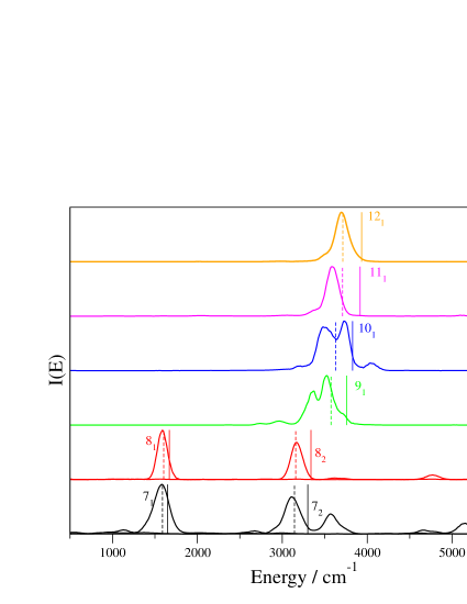
Figure 2: MC-DC-SCIVR vibrational spectra of bendings and stretches of the water dimer based on 5 trajectories per subspace. The vertical solid lines indicate the harmonic estimates, while the dashed vertical lines the MultiMode results. The bending fundamental and overtone signals were obtained by tuning the reference state according to Eq. (14).

III.2 Water Trimer (H₂O)₃

The water trimer is made of 21 vibrational degrees of freedom, 3 of which are bendings and 6 are OH stretches. In order to reduce the computational burden, we employed a version of the three body potential which is, as anticipated, very fast to compute and retains quite well the accuracy of the original WHBB 3-body potential. A first analysis of the trimer is obtained by looking at its Hessian threshold trend. We observe that employing the same threshold value used for the dimer would lead to label all vibrational modes as indepedent ones, reflecting the decrement in magnitude of the off-diagonal elements of the trimer Hessian. Furthermore, for the trimer, three plateau can be clearly identified at maximum subspace dimensionality values of 8, 6 and 1. However, similarly to the dimer case, spectra projected onto high-dimensional subspaces cannot be well resolved and the maximum subspace dimensionality still consistent with a resolved spectrum is 3. For this reason and to keep working with subspaces as high dimensional as possible, we used a threshold value for the trimer equal to $1.5\cdot 10^{-5}$. The relevant 9-dimensional space has been consequently divided into mono, bi- and tri-dimensional subspaces. In particular, modes 17,18,19 have been enrolled into a 3-dimensional subspace, while modes 16 and 20 into a bidimensional one. Generation of the initial conditions and the subsequent dynamics have been performed according to the methodology already described for the dimer.

Table 2: Main fundamental vibrational frequencies of the water trimer, in $\text{c$m^{-1}$}.$ Labels are the same as in Table (1). Last column shows classical-like results from Eq. (17) based on the Fourier transform (FT) of the velocity-velocity autocorrelation function (C_vv). MAE values are relative to MultiMode (MM) results.

Index	HO	MM58	LMM58	DC SCIVR10k	MC-DC SCIVR${}_{\text{10trajs,multmin}}$	MC-DC SCIVR${}_{\text{1 traj}}$	$FT(\text{$C_{vv}$})$
$13_{1}$	1661	1597	1602	1584	1575	1534	1520
$14_{1}$	1664	1600	1614	1595	1637	1528	1520
$15_{1}$	1681	1623	1615	1627	1634	1530	1516
$16_{1}$	3664	3486	3489	3440	3386	3426	3536
$17_{1}$	3703	3504	3500	3450	3400	3547	3548
$18_{1}$	3711	3514	3510	3247	3380	3151	3480
$19_{1}$	3911	3709	3718	3640	3610	3706	3676
$20_{1}$	3916	3715	3718	3700	3675	3652	3697
$21_{1}$	3918	3720	3719	3736	3760	3684	3640
MAE	151	-	6	54	65	88	58

Table (2) shows our DC-SCIVR (based on 10,000 trajectories, 30,000 atomic time units long) and MC-DC-SCIVR results compared to the MultiMode and Local Monomer Model ones.⁵⁸ Once again, a single trajectory is insufficient to recover the correct semiclassical spectral features, and a preliminary exploration of the Potential Energy Surface is required for application of MC-DC SCIVR. We found nine different local minima very close in energy to the global one. We repeated the same MC-DC-SCIVR procedure described in the dimer section, running in this case 10 trajectories for each subspace, each one centered on a different minimum (global or local).

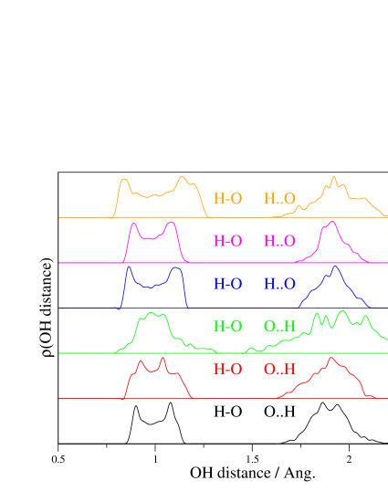
Figure 3: Distribution of the OH distance during a dynamics where the i-th mode is initially excited in order to enhance its motion. The left side of the panel reports the OH distance of bound atoms, while in the right side of the panel the distribution of OH involved in the hydrogen bonds (O…H) is presented. The different colors refer to different modes.

The energy range of the vibrational levels is very similar between the two oligomers so far investigated, with the trimer having the bending frequencies slightly blue shifted with respect to the dimer, in agreement with results reported in the literature.³²; ¹¹³; ⁶⁰ Larger differences may be found for the OH stretchings which are in general red shifted with respect to the dimer. Semiclassical results show a strong red-shift of mode 18 and, more mildly, of modes 16 and 17 with respect to MM values, which is responsible for most of the MAE values reported in Table (2). The red shift found with semiclassical calculations can be explained by looking at Figure (3), where for modes 16-21 we compare the distributions of intramolecular (O-H) distances to (O..H) distances involved in the hydrogen bonds along trajectories with mode-specific excitation. Modes 19 and 20 seem to be not affected at all by long range interactions, as expected by their free OH stretching nature. Mode 21 is also a high-frequency free stretch. It has a broader distribution of the intramolecular O-H distance which contributes to the appearance of a tail at shorter distances for the intermolecular O..H distance. The intramolecular motion for mode 21 is dominant, while the tail of the distribution is not directional and hydrogen bonding is not effective. On the opposite, for modes 16, 17, 18 (with particular emphasis for the latter) the short O..H distances are related to a strong dynamical hydrogen interaction. Because of it, a bond weakening is expected resulting into a red-shift of the vibrational frequency. This is clearly seen upon comparison with MM results. The dynamical effect that influences modes involved in hydrogen bonds justifies a large part of the 54 (or 65 for MC-DC-SCIVR) wavenumbers of MAE with respect to MM values, since if only bending and free OH frequencies (which are not affected by hydrogen bonding) are compared, then the MAE reduces to 20 (or 40 for MC-DC-SCIVR) cm^-1. As anticipated, single-trajectory MC-DC-SCIVR simulations are not reliable and the major improvement we have found upon moving to a MC-DC-SCIVR approach based on multiple minima (and trajectories) concerns the low-energy red-shifted OH stretches because of the non-local hydrogen interactions. Such non-local behavior could justify the differences that arise between our results and MM ones, while another source of discrepancy might come from the fact we employed a different (even if similar) PES for the three-body interaction. Furthermore, as already pointed out for the dimer, these low frequency OH stretches show much more complex spectral features with respect to modes 13-16 and 19-21 owing to the interactions with the bending overtones (which are in the same energy range) or other stretches as depicted by Figure (4). Figure (4) shows the computed spectra employing the MC-DC-SCIVR approach (solid lines) and reports MM (dashed vertical lines) and harmonic (solid vertical lines) frequencies. Bending overtones are very sensitive to the energy of the trajectories employed in the semiclassical calculations and they cannot be precisely detected when employing a dynamics energetically tailored on the OH stretchings, and this adds to the complexity of the resulting spectra. In particular, mode 18 presents several low-frequency spectral features due to the overtone bendings and a peak which is blue shifted compared to the MM frequency and that is due to mode 19.

To point out the importance of a semiclassical approach we have also computed classical-like spectra obtained from the Fourier transform of velocity-velocity correlation functions. The trajectory starting conditions were sampled using the same strategy adopted for semiclassical simulations with the aim to make the comparison between the different approaches as straightforward as possibile. In the classical-like case, 5,000 classical trajectories for each fundamental mode were enough to get reliable results. We notice that the classical estimates for the three OH bending frequencies are substantially red-shifted with respect to MM, LMM, and DC SCIVR ones, while free OH stretches are found in better agreement. Looking at modes 16-18, the red-shift is less prominent when the outcomes of classical-like simulations are compared with DC SCIVR results. Furthermore, as expected, no overtone features are present in these classical-like spectra.

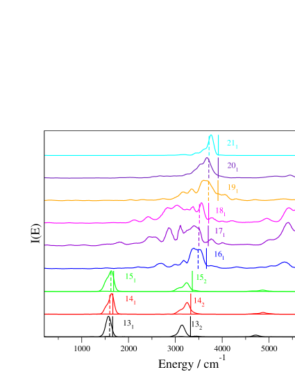
Figure 4: Vibrational spectra of the water trimer. The solid lines refer to MC-DC-SCIVR simulations based on 10 trajectories for each subspace; vertical solid lines indicate the harmonic estimates, while dashed ones the benchmark MultiMode values. The bending fundamental and overtone signals were obtained by tuning the reference state according to Eq. (14).

Finally, we compare in Table (3) our results to available experimental data, and find low discrepancies (about 30 cm^-1 on average) within the typical semiclassical accuracy. As anticipated, classical-like results are off the mark in the bending region.

Table 3: Experimental vibrational frequencies available for the water trimer, in c$m^{-1}$, and calculated ones. Experimental data are not assigned to a specific vibrational mode, so for each theoretical approach the closest frequency has been chosen for comparison. Labels are the same as in previous Tables. MAE is the mean absolute error referred to experimental data.

	Exp.114; 113	MM58	LMM58	DC SCIVR${}_{\text{10k}}$	MC-DC SCIVR${}_{\text{10trajs,multmin}}$	$FT(\text{$C_{vv}$})$
	1608	1597	1602	1584	1575	1520
	1609	1600	1614	1595	1637	1520
	1629	1623	1615	1627	1634	1516
	3533	3514	3510	3640	3610	3536
	3726	3720	3719	3736	3760	3697
MAE	-	10	11	31	35	64

III.3 Water Hexamer prism (H₂O)₆

In this Section we explore the vibrational features of the water hexamer prism. It presents 48 degrees of freedom, 18 of which are bendings and OH stretches. Similarly to what happens moving from the dimer to the trimer, the magnitude of interactions becomes less intense going from the trimer to the hexamer. Indeed, with the same Hessian threshold value adopted for the trimer, all the modes of the hexamer have been treated independently, with the exception of a couple of modes (number 35 and 45) which have been still enrolled into a bi-dimensional subspace.

We computed the hexamer DC-SCIVR spectra with 5,000 trajectories per subspace, and, similarly to the case of the dimer and trimer, we also checked the reliability of a MC-DC-SCIVR approach based on just a few trajectories. However, from our damped dynamics simulations it was soon evident that too many local minima had to be taken into consideration. Running a trajectory from each minimum would have not provided a real computational advantage over DC-SCIVR, so we introduced a different approach to select the most relevant minima for our calculations.

We adopted a strategy inspired by Habershon’s recent work on correlation distributions.¹¹⁵ As anticipated, the many-body PES of the hexamer is characterized by several local minima, very close in energy to each other. To assess the “vicinity” of each minimum to the global one, we chose a connection criterion based on structural considerations. Specifically, we introduced a correlation parameter computed as a sum of molecular distances. In fact, by defining a proper set of distances $\left\{d_{i}\right\}_{i=1,\ldots,N_{distances}}$ between the atoms, the correlation parameter $\sigma^{2}$ can be calculated as

$$\sigma^{2}=\sum_{i=1}^{N_{distances}}(d-d_{i}^{ref})^{2},$$ (18)

where $d_{i}^{ref}$ is the i-th distance calculated at the global minimum geometry. In the set of distances we included the length of OH bonds for each of the six monomers plus the O-O distances of adjacent oxygen atoms. By looking at Eq. (18) it is expected that minima very correlated to the global one have $\sigma^{2}\rightarrow 0$, while higher values identify less correlated wells.

We took into consideration $\sigma^{2}$ values up to 0.011 Ų, which is enough to cover more than 80% of the located local minima. Those which are further away from the global minimum (in $\sigma^{2}$ terms) are expected to contribute less significantly to the spectral features, and are neglected. Figure (5) shows the correlation distribution as a function of $\sigma^{2}$ for different sets of damped-dynamics trajectories employed. As in previous cases, the initial conditions of the damped trajectories are sampled by means of a Husimi distribution around the PES global minimum, and a damping factor equal to 0.99 is adopted. Peaks in the distribution, sampled along the $\sigma^{2}$ range studied, are used to select the most relevant minima for the MC-SCIVR calculations.

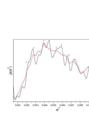
Figure 5: Correlation distribution between the global minimum and the local minima found by exploring the hexamer many-body PES. The plots report the results for 1,000 (black) and 10,000 (red) damped-dynamics trajectories. Data have been interpolated by means of a cubic spline. The black asterisks represent the correlation peaks corresponding to the minima employed in the MC-DC-SCIVR calculations.

Table 4: Vibrational frequencies of the water hexamer prism, in $\text{c$m^{-1}$}.$ The first column refers to the mode-excitation label; the second column is the harmonic estimate; the third column reports the Local Monomer Model results; from the fourth column on, the semiclassical values are listed. The MC-DC-SCIVR simulation based on 11 trajectories has been performed upon selection of 10 local minima from the correlation distribution. MAE values are referred to LMM ones.

Index	HO	LMM58	DC SCIVR${}_{\text{5k}}$	MC-DC SCIVR11trajs,multmin	MC-DC SCIVR1traj
$31_{1}$	1661	1606	1617	1602	1606
$32_{1}$	1672	1612	1623	1620	1592
$33_{1}$	1676	1620	1622	1622	1588
$34_{1}$	1701	1633	1664	1636	1682
$35_{1}$	1715	1654	1661	1640	1684
$36_{1}$	1739	1677	1715	1712	1722
$37_{1}$	3377	3092	2925	2956	3011
$38_{1}$	3494	3256	3052	3060	3012
$39_{1}$	3619	3372	3182	3168	2940
$40_{1}$	3638	3442	3516	3395	3198
$41_{1}$	3714	3482	3573	3556	3200
$42_{1}$	3735	3521	3640	3616	3500
$43_{1}$	3792	3579	3592	3606	3680
$44_{1}$	3809	3588	3580	3574	3608
$45_{1}$	3827	3630	3678	3650	3602
$46_{1}$	3915	3697	3771	3610	3578
$47_{1}$	3923	3706	3698	3750	3768
$48_{1}$	3925	3728	3677	3712	3700
MAE	169	-	64	57	102

Table (4) shows our results compared to the Local Monomer Model ones.⁵⁸ Vibrations are predicted by LMM at lower frequencies than the typical OH stretching region, approximately in the range between 3,100 and 3,300 cm^-1. Some semiclassical results were found in the 2,900-3,100 cm^-1 region of the spectrum. Therefore our dynamics-based results for the lower-frequency stretches are red shifted with respect to the time-independent ones. We ascribe the main reason for this discrepancy to the different impact of hydrogen interactions, which weaken such OH bonds. In a dynamical approach, the effect of hydrogen bonding is enhanced, as already evinced for the trimer. A further evidence of this is reported in Figure (6) where we compare the distributions of intramolecular (O-H) distances to (O..H) distances involved in the hydrogen bonds for modes 37-41 along trajectories with specific mode excitation. Modes 37-39, which are semiclassically the most red-shifted ones, present a more prominent tail at short O..H distances with respect to modes 40-41, which are not red shifted. These features point to a stronger OH..O hydrogen interaction for modes 37-39 than for the other stretches. Consequently, the corresponding OH bonds are weakened and their frequencies red shifted. MAE values relative to the LMM ones are around 60 cm^-1for DC-SCIVR and MC-DC-SCIVR based on 11 trajectories, while the MAE is substantially higher (~100 cm^-1) when a single trajectory is employed. These values are much lower if only modes not involved in hydrogen bonding, i.e. modes 31-36 and 43-48, are considered. In fact the MAE decreases to 25 cm^-1for DC SCIVR, and to 22 cm^-1for MC-DC SCIVR with 11 trajectories.

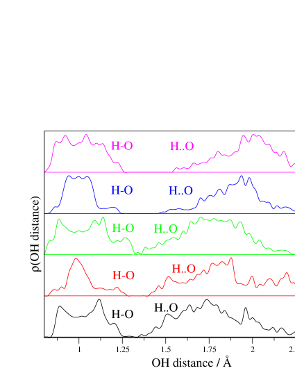
Figure 6: Distribution of the OH distance during a dynamics where the i-th mode is initially excited in order to enhance its motion. The left side of the panel reports the OH distance of bound atoms, while in the right side of the panel the distribution of OH involved in the hydrogen bonds (O…H) is presented. The different colors refer to different modes.

Figures (7), (8), and (9) show the spectra computed for the hexamer employing the MC-DC-SCIVR approach with 11 trajectories (solid line) together with the LMM (dashed vertical lines) and harmonic (solid vertical lines) frequency estimates. Specifically, in Figure (7) the six bendings and their overtones are reported, while Figures (8) and (9) are dedicated to the low-frequency and free OH stretches respectively. If, for bendings, spectral features are well resolved, peaks associated to the stretches are instead broader and have a more complex shape due to the intermode couplings involving both stretches and overtones of bendings. This was also observed in the trimer and it is evident in the hexamer too. In particular, power spectra of modes 39 and 40 present a double peak feature due to the coupling between these two modes. A similar instance occurs for spectra of modes 41 and 42 which, in addition, show a shoulder at the frequency of mode 37. The effects of coupling fade away when moving to the free OH stretches, a characteristic which has been already found in the trimer.

Figure 7: Vibrational spectra of the water hexamer prisms in the bending region. The solid lines refer to MC-DC-SCIVR simulations based on 11 trajectories for each subspace; vertical solid lines indicate the harmonic estimates, while dashed ones the Local Monomer values. The bending fundamental and overtone signals were obtained by tuning the reference state according to Eq. (14).

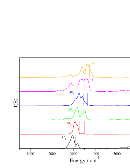
Figure 8: Vibrational spectra of the water hexamer prism in the OH stretching region. The solid lines refer to MC-DC-SCIVR simulations based on 11 trajectories for each subspace; vertical solid lines indicate the harmonic estimates, while dashed ones the Local Monomer values.

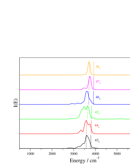
Figure 9: Vibrational spectra of the water hexamer prism in the free OH stretching region. The solid lines refer to MC-DC-SCIVR simulations based on 11 trajectories for each subspace; vertical solid lines indicate the harmonic estimates, while dashed ones the Local Monomer values.

In summary, the semiclassical information about the hexamer energy levels based on thousands of trajectories can be basically regained by means of a MC-DC-SCIVR treatment that employs just 11 selected trajectories. A single-trajectory approach is instead not enough to recover the correct spectral features due to the strong influence of local minima similar in both energy and connectivity to the global one. Therefore, our MC-DC-SCIVR approach is very promising for dealing with higher-dimensional clusters for which a DC-SCIVR calculation is out of reach as in the case of the water decamer $\left(\text{H}_{2}\text{O}\right)_{10}$.

III.4 Water Decamer (H₂O)₁₀

Our last application concerns the water decamer which has 10 bendings and 20 OH stretches, and a total of 84 vibrational degrees of freedom. Due to the computational overhead of the simulations, for the decamer we only performed MC-DC-SCIVR calculations based on multiple trajectories starting from a set of minima located by means of the damped-dynamics approach. We identified several minima on the surface and calculated a correlation distribution dependent on intramolecular OH distances and OO distances of adjacent monomers according to Eq. (18), from which we extracted the 10 most relevant local minima. By employing the same Hessian threshold value adopted for the trimer and the hexamer, all 30 degrees of freedom have been treated as independent ones. This is in agreement with the trend of weakening interactions between vibrational modes associated with an increase in the dimensionality of the system. For each subspace we performed our MC-DC-SCIVR calculations based on 11 trajectories initiated from the global minimum and the 10 chosen local minima. Results are reported in Table (5) which shows a comparison of the decamer semiclassical fundamental frequencies with the corresponding values calculated with the Local Monomer Model.⁵⁸

Table 5: Fundamental frequencies of vibration for the water decamer ($cm^{-1}$). HO is the label for the harmonic frequencies; LMM are the Local Monomer Model results; MC-DC-SCIVR refers to our semiclassical estimates.

HO	LMM58	MC-DC-SCIVR11 trajs, multmin		HO	LMM58	MC-DC-SCIVR11 trajs, multmin
1670	1600	1590		3571	3382	3337
1675	1602	1624		3659	3417	3379
1678	1608	1624		3666	3419	3400
1686	1609	1628		3676	3420	3406
1692	1617	1660		3682	3429	3448
1712	1647	1663		3727	3518	3492
1713	1664	1674		3741	3525	3496
1720	1665	1690		3756	3534	3522
1738	1669	1708		3774	3566	3532
1748	1691	1714		3781	3568	3565
3335	3013	2936		3914	3706	3640
3352	3036	3006		3920	3734	3668
3383	3046	3022		3924	3736	3672
3387	3050	3052		3925	3741	3680
3554	3286	3121		3926	3744	3800

In this case we observe that our results for the bendings are generally in good agreement with LMM ones with a MAE equal to 36 wavenumbers. Both MC-DC-SCIVR and LMM predict more red-shifted stretches than in the case of the smaller clusters, but they are in closer agreement with respect to the trimer or the hexamer.

IV Summary and Conclusions

In this paper we have presented a semiclassical investigation of the vibrational features of some water clusters ranging from the dimer to the decamer by means of our recently established Divide-and-Conquer semiclassical approach. Semiclassical simulations employ several thousand classical trajectories to reach convergence of results, but a computationally-cheaper MC-DC-SCIVR approach based on few, selected trajectories was demonstrated to provide quite acceptable results. The caveat here is that, differently from other molecular systems studied in the past, a single-minimum/single-trajectory semiclassical calculation is usually not accurate. Therefore, we have explored the potential energy surface looking for local minima and presented a way to select them according to their “resemblance” to the global minimum and their expected contribution to the calculations. The application of semiclassical methods to water clusters demonstrates that these techniques can be employed also for large $\left(\text{H}_{2}\text{O}\right)_{n}$ ones as well as for rather floppy systems, and not only for quite rigid ones. The divide-and-conquer method is able to simplify the full-dimensional problem recovering part of the interactions between the low-dimensional subspaces thanks to the maintained full-dimensional nature of the trajectories on which the subspace calculations are based. Spectral features though are very sensitive to intermode couplings and multiple peak structures are often present especially in the case of low frequency stretches. Furthermore, vibrational angular momentum due to the floppy nature of the system contributes to increase the width of peaks, which is substantially larger than what is commonly found in semiclassical calculations of single molecules.

Results show that the outcomes of experiments and previous theoretical studies are regained with quantitative agreement for bendings and free OH stretches, while frequencies of OH stretches influenced by hydrogen-bond interactions are red shifted with respect to the estimates provided by other theoretical approaches. This can be clearly seen in the assignment of the trimer experimental frequency at 3533 cm^-1. We assign it semiclassically to mode 19, while VCI calculations yield a closer estimate for the frequency of mode 18, and classical-like simulations point to mode 16. The difference between semiclassical and classical-like estimates is evident and confirms the need to undertake a semiclassical approach able to regain quantum effects. The presence of a set of semiclassical frequencies around 3,000 cm^-1 for the hexamer and the decamer is consistent with previous studies even if the red shift is more accentuated in our simulations. This is due to dynamical effects (confirmed by the short-distance tails of the O..H distance distributions for modes involved in hydrogen bonds) and to the multi-reference nature of the semiclassical approach. Compared to the isolated water molecule, bending frequencies are more and more blue shifted and low-frequency stretches more and more red-shifted as the cluster size increases. Agreement between semiclassical and VCI calculations for modes in the red-shift region is better for the decamer than for smaller clusters.

SUPPLEMENTARY MATERIAL

See Supplementary Material for the new 3-body water-water-water PES employed in this work.

References

- Wu and Voth (2003) Y. Wu and G. A. Voth, Biophys. J. 85, 864 (2003).
- Smondyrev and Voth (2002) A. M. Smondyrev and G. A. Voth, Biophys. J. 82, 1460 (2002).
- Petersen et al. (2005) M. K. Petersen, F. Wang, N. P. Blake, H. Metiu, and G. A. Voth, J. Phys. Chem. B 109, 3727 (2005).
- Mohammed et al. (2005) O. F. Mohammed, D. Pines, J. Dreyer, E. Pines, and E. T. Nibbering, Science 310, 83 (2005).
- Riccardi et al. (2006) D. Riccardi, P. Koenig, X. Prat-Resina, H. Yu, M. Elstner, T. Frauenheim, and Q. Cui, J. Am. Chem. Soc. 128, 16302 (2006).
- Wolke et al. (2016) C. T. Wolke, J. A. Fournier, L. C. Dzugan, M. R. Fagiani, T. T. Odbadrakh, H. Knorke, K. D. Jordan, A. B. McCoy, K. R. Asmis, and M. A. Johnson, Science 354, 1131 (2016).
- Marx (2006) D. Marx, Chem. Phys. Chem. 7, 1848 (2006).
- Feyereisen, Feller, and Dixon (1996) M. W. Feyereisen, D. Feller, and D. A. Dixon, J. Phys. Chem. 100, 2993 (1996).
- Poole et al. (1994) P. H. Poole, F. Sciortino, T. Grande, H. E. Stanley, and C. A. Angell, Phys. Rev. Lett. 73, 1632 (1994).
- Liu et al. (1996) K. Liu, M. Brown, C. Carter, R. Saykally, et al., Nature 381, 501 (1996).
- Xantheas (2000) S. S. Xantheas, Chem. Phys. 258, 225 (2000).
- Liu, Cruzan, and Saykally (1996) K. Liu, J. Cruzan, and R. Saykally, Science 271, 929 (1996).
- Pfeilsticker et al. (2003) K. Pfeilsticker, A. Lotter, C. Peters, and H. Bösch, Science 300, 2078 (2003).
- Vöhringer-Martinez et al. (2007) E. Vöhringer-Martinez, B. Hansmann, H. Hernandez, J. Francisco, J. Troe, and B. Abel, Science 315, 497 (2007).
- Yu and Bowman (2017) Q. Yu and J. M. Bowman, J. Am. Chem. Soc. 139, 10984 (2017).
- Conte, Qu, and Bowman (2015) R. Conte, C. Qu, and J. M. Bowman, J. Chem. Theory Comput. 11, 1631 (2015).
- Qu et al. (2015) C. Qu, R. Conte, P. L. Houston, and J. M. Bowman, Phys. Chem. Chem. Phys. 17, 8172 (2015).
- Homayoon et al. (2015) Z. Homayoon, R. Conte, C. Qu, and J. M. Bowman, J. Chem. Phys. 143, 084302 (2015).
- Mancini and Bowman (2013) J. S. Mancini and J. M. Bowman, J. Chem. Phys. 138, 121102 (2013).
- Mancini and Bowman (2014) J. S. Mancini and J. M. Bowman, J. Phys. Chem. Lett. 5, 2247 (2014).
- Samanta et al. (2016) A. K. Samanta, Y. Wang, J. S. Mancini, J. M. Bowman, and H. Reisler, Chem. Rev. 116, 4913 (2016).
- Kamarchik et al. (2014) E. Kamarchik, D. Toffoli, O. Christiansen, and J. M. Bowman, Spectrochimica Acta Part A: Molecular and Biomolecular Spectroscopy 119, 59 (2014).
- Kamarchik, Wang, and Bowman (2011) E. Kamarchik, Y. Wang, and J. M. Bowman, J. Chem. Phys. 134, 114311 (2011).
- Kamarchik and Bowman (2010) E. Kamarchik and J. M. Bowman, J. Phys. Chem. A 114, 12945 (2010).
- Wang, Bowman, and Kamarchik (2016) Y. Wang, J. M. Bowman, and E. Kamarchik, J. Chem. Phys. 144, 114311 (2016).
- Paul et al. (1997) J. Paul, C. Collier, R. Saykally, J. Scherer, and A. O’keefe, J. Phys. Chem. A 101, 5211 (1997).
- Bouteiller and Perchard (2004) Y. Bouteiller and J. Perchard, Chem. Phys. 305, 1 (2004).
- Buck and Huisken (2000) U. Buck and F. Huisken, Chem. Rev. 100, 3863 (2000).
- Paul et al. (1998) J. Paul, R. Provencal, C. Chapo, A. Petterson, and R. Saykally, J. Chem. Phys. 109, 10201 (1998).
- Lakshminarayanan, Suresh, and Ghosh (2005) P. Lakshminarayanan, E. Suresh, and P. Ghosh, J. Am. Chem. Soc. 127, 13132 (2005).
- Steinbach et al. (2004) C. Steinbach, P. Andersson, M. Melzer, J. Kazimirski, U. Buck, and V. Buch, Phy. Chem. Chem. Phys. 6, 3320 (2004).
- Paul et al. (1999) J. Paul, R. Provencal, C. Chapo, K. Roth, R. Casaes, and R. Saykally, J. Phys. Chem. A 103, 2972 (1999).
- Hirabayashi and Yamada (2005) S. Hirabayashi and K. M. Yamada, J. Chem. Phys. 122, 244501 (2005).
- Buck et al. (1998) U. Buck, I. Ettischer, M. Melzer, V. Buch, and J. Sadlej, Phys. Rev. Lett. 80, 2578 (1998).
- Yoo et al. (2010) S. Yoo, E. Apra, X. C. Zeng, and S. S. Xantheas, J. Phys. Chem. Lett. 1, 3122 (2010).
- Bulusu et al. (2006) S. Bulusu, S. Yoo, E. Apra, S. Xantheas, and X. C. Zeng, J. Phys. Chem. A 110, 11781 (2006).
- Xantheas and Dunning Jr (1993) S. S. Xantheas and T. H. Dunning Jr, J. Chem. Phys. 98, 8037 (1993).
- Maheshwary et al. (2001) S. Maheshwary, N. Patel, N. Sathyamurthy, A. D. Kulkarni, and S. R. Gadre, J. Phys. Chem. A 105, 10525 (2001).
- Wales and Hodges (1998) D. J. Wales and M. P. Hodges, Chem. Phys. Lett. 286, 65 (1998).
- Xantheas, Burnham, and Harrison (2002) S. S. Xantheas, C. J. Burnham, and R. J. Harrison, J. Chem. Phys. 116, 1493 (2002).
- Xantheas (1995) S. S. Xantheas, J. Chem. Phys. 102, 4505 (1995).
- Bowman et al. (2010) J. M. Bowman, B. Braams, S. Carter, C. Chen, G. Czakó, B. Fu, X. Huang, E. Kamarchik, A. Sharma, B. Shepler, et al., J. Phys. Chem. Lett. 1, 1866 (2010).
- Wang et al. (2012) Y. Wang, V. Babin, J. M. Bowman, and F. Paesani, J. Am. Chem. Soc. 134, 11116 (2012).
- Liu, Wang, and Bowman (2012) H. Liu, Y. Wang, and J. M. Bowman, J. Phys. Chem. Lett. 3, 3671 (2012).
- Chng et al. (2012) L. C. Chng, A. K. Samanta, G. Czako, J. M. Bowman, and H. Reisler, J. Am. Chem. Soc. 134, 15430 (2012).
- Wang and Bowman (2013) Y. Wang and J. M. Bowman, J. Phys. Chem. Lett. 4, 1104 (2013).
- Babin and Paesani (2013) V. Babin and F. Paesani, Chem. Phys. Lett. 580, 1 (2013).
- Medders and Paesani (2013) G. R. Medders and F. Paesani, J. Chem. Theory Comput. 9, 4844 (2013).
- Liu, Wang, and Bowman (2015) H. Liu, Y. Wang, and J. M. Bowman, J. Chem. Phys. 142, 194502 (2015).
- Richardson et al. (2016) J. O. Richardson, C. Pérez, S. Lobsiger, A. A. Reid, B. Temelso, G. C. Shields, Z. Kisiel, D. J. Wales, B. H. Pate, and S. C. Althorpe, Science 351, 1310 (2016).
- Partridge and Schwenke (1997) H. Partridge and D. W. Schwenke, J. Chem. Phys. 106, 4618 (1997).
- Burnham et al. (1999) C. J. Burnham, J. Li, S. S. Xantheas, and M. Leslie, J. Chem. Phys. 110, 4566 (1999).
- Burnham and Xantheas (2002) C. J. Burnham and S. S. Xantheas, J. Chem. Phys. 116, 5115 (2002).
- Fanourgakis and Xantheas (2006) G. S. Fanourgakis and S. S. Xantheas, J. Phys. Chem. A 110, 4100 (2006).
- Huang et al. (2008) X. Huang, B. J. Braams, J. M. Bowman, R. E. Kelly, J. Tennyson, G. C. Groenenboom, and A. van der Avoird, J. Chem. Phys. 128, 034312 (2008).
- Fanourgakis and Xantheas (2008) G. S. Fanourgakis and S. S. Xantheas, J. Chem. Phys. 128, 074506 (2008).
- Shank et al. (2009) A. Shank, Y. Wang, A. Kaledin, B. J. Braams, and J. M. Bowman, J. Chem. Phys. 130, 144314 (2009).
- Wang and Bowman (2011) Y. Wang and J. M. Bowman, J. Chem. Phys. 134, 154510 (2011).
- Wang et al. (2011) Y. Wang, X. Huang, B. C. Shepler, B. J. Braams, and J. M. Bowman, J. Chem. Phys. 134, 094509 (2011).
- Wang and Bowman (2016) Y. Wang and J. M. Bowman, Phys. Chem. Chem. Phys. 18, 24057 (2016).
- Xantheas (1994) S. S. Xantheas, J. Chem. Phys. 100, 7523 (1994).
- Gregory and Clary (1995) J. K. Gregory and D. C. Clary, J. Chem. Phys. 103, 8924 (1995).
- Wang et al. (2009) Y. Wang, B. C. Shepler, B. J. Braams, and J. M. Bowman, J. Chem. Phys. 131, 054511 (2009).
- Heller (1981a) E. J. Heller, Acc. Chem. Res. 14, 368 (1981a).
- Shao and Makri (1999) J. Shao and N. Makri, J. Phys. Chem. A 103, 7753 (1999).
- Miller (2001) W. H. Miller, J. Phys. Chem. A 105, 2942 (2001).
- Shalashilin and Child (2004) D. V. Shalashilin and M. S. Child, Chem. Phys. 304, 103 (2004).
- Pollak (2007) E. Pollak, “The Semiclassical Initial Value Series Representation of the Quantum Propagator,” in Quantum Dynamics of Complex Molecular Systems, edited by D. A. Micha and I. Burghardt (Springer Berlin Heidelberg, Berlin, Heidelberg, 2007) pp. 259–271.
- Tatchen and Pollak (2009) J. Tatchen and E. Pollak, J. Chem. Phys. 130, 041103 (2009).
- Conte and Pollak (2010) R. Conte and E. Pollak, Phys. Rev. E 81, 036704 (2010).
- Conte and Pollak (2012) R. Conte and E. Pollak, J. Chem. Phys. 136, 094101 (2012).
- Wehrle, Oberli, and Vaníček (2015) M. Wehrle, S. Oberli, and J. Vaníček, J. Phys. Chem. A 119, 5685 (2015).
- Antipov, Ye, and Ananth (2015) S. V. Antipov, Z. Ye, and N. Ananth, J. Chem. Phys. 142, 184102 (2015).
- Chapman, Cheng, and Cina (2011) C. T. Chapman, X. Cheng, and J. A. Cina, J. Phys. Chem. A 115, 3980 (2011).
- Nakamura et al. (2016) H. Nakamura, S. Nanbu, Y. Teranishi, and A. Ohta, Phys. Chem. Chem. Phys. 18, 11972 (2016).
- Bonnet and Rayez (2004) L. Bonnet and J.-C. Rayez, Chem. Phys. Lett. 397, 106 (2004).
- Kaledin and Miller (2003a) A. L. Kaledin and W. H. Miller, J. Chem. Phys. 118, 7174 (2003a).
- Kaledin and Miller (2003b) A. L. Kaledin and W. H. Miller, J. Chem. Phys. 119, 3078 (2003b).
- Di Liberto and Ceotto (2016) G. Di Liberto and M. Ceotto, J. Chem. Phys. 145, 144107 (2016).
- Conte, Aspuru-Guzik, and Ceotto (2013) R. Conte, A. Aspuru-Guzik, and M. Ceotto, J. Phys. Chem. Lett. 4, 3407 (2013).
- Ceotto, Tantardini, and Aspuru-Guzik (2011) M. Ceotto, G. F. Tantardini, and A. Aspuru-Guzik, J. Chem. Phys. 135, 214108 (2011).
- Ceotto et al. (2011) M. Ceotto, S. Valleau, G. F. Tantardini, and A. Aspuru-Guzik, J. Chem. Phys. 134, 234103 (2011).
- Ceotto et al. (2009a) M. Ceotto, S. Atahan, G. F. Tantardini, and A. Aspuru-Guzik, J. Chem. Phys. 130, 234113 (2009a).
- Ceotto et al. (2009b) M. Ceotto, S. Atahan, S. Shim, G. F. Tantardini, and A. Aspuru-Guzik, Phys. Chem. Chem. Phys. 11, 3861 (2009b).
- Ceotto, Dell‘ Angelo, and Tantardini (2010) M. Ceotto, D. Dell‘ Angelo, and G. F. Tantardini, J. Chem. Phys. 133, 054701 (2010).
- Tamascelli et al. (2014) D. Tamascelli, F. S. Dambrosio, R. Conte, and M. Ceotto, J. Chem. Phys. 140, 174109 (2014).
- Buchholz, Grossmann, and Ceotto (2016) M. Buchholz, F. Grossmann, and M. Ceotto, J. Chem. Phys. 144, 094102 (2016).
- Buchholz, Grossmann, and Ceotto (2017) M. Buchholz, F. Grossmann, and M. Ceotto, The Journal of Chemical Physics 147, 164110 (2017).
- Zhuang et al. (2013) Y. Zhuang, M. R. Siebert, W. L. Hase, K. G. Kay, and M. Ceotto, J. Chem. Theory Comput. 9, 54 (2013).
- Ceotto, Zhuang, and Hase (2013) M. Ceotto, Y. Zhuang, and W. L. Hase, J. Chem. Phys. 138, 054116 (2013).
- Ceotto, Di Liberto, and Conte (2017) M. Ceotto, G. Di Liberto, and R. Conte, Phys. Rev. Lett. 119, 010401 (2017).
- Liberto, Conte, and Ceotto (2018) G. D. Liberto, R. Conte, and M. Ceotto, J. Chem. Phys. 148, 014307 (2018).
- Conte, Houston, and Bowman (2014) R. Conte, P. L. Houston, and J. M. Bowman, J. Chem. Phys. 140, 151101 (2014).
- Houston, Conte, and Bowman (2015) P. L. Houston, R. Conte, and J. M. Bowman, J. Phys. Chem. A 119, 4695 (2015).
- Conte, Houston, and Bowman (2015) R. Conte, P. L. Houston, and J. M. Bowman, J. Phys. Chem. A 119, 12304 (2015).
- Houston, Conte, and Bowman (2016) P. L. Houston, R. Conte, and J. M. Bowman, J. Phys. Chem. A 120, 5103 (2016).
- Feynman and Hibbs (1965) R. P. Feynman and A. R. Hibbs, Quantum mechanics and path integrals (McGraw-Hill, 1965).
- Tannor (2007) D. J. Tannor, Introduction to quantum mechanics (University Science Books, 2007).
- Van Vleck (1928) J. H. Van Vleck, Proc. Natl. Acad. Sci. 14, 178 (1928).
- Miller (1970) W. H. Miller, J. Chem. Phys. 53, 3578 (1970).
- Heller (1981b) E. J. Heller, J. Chem. Phys. 75, 2923 (1981b).
- Heller (1991) E. J. Heller, J. Chem. Phys. 94, 2723 (1991).
- Herman and Kluk (1984) M. F. Herman and E. Kluk, Chem. Phys. 91, 27 (1984).
- Wang, Manolopoulos, and Miller (2001) H. Wang, D. E. Manolopoulos, and W. H. Miller, J. Chem. Phys. 115, 6317 (2001).
- Kay (1994a) K. G. Kay, J. Chem. Phys. 101, 2250 (1994a).
- Kay (1994b) K. G. Kay, J. Chem. Phys. 100, 4432 (1994b).
- Hinsen and Kneller (2000) K. Hinsen and G. R. Kneller, Mol. Simul. 23, 275 (2000).
- Harland and Roy (2003) B. B. Harland and P.-N. Roy, J. Chem. Phys. 118, 4791 (2003).
- Gelabert et al. (2000) R. Gelabert, X. Giménez, M. Thoss, H. Wang, and W. H. Miller, J. Phys. Chem. A 104, 10321 (2000).
- Gabas, Conte, and Ceotto (2017) F. Gabas, R. Conte, and M. Ceotto, J. Chem. Theory Comput. 13, 2378 (2017).
- Markovich et al. (2016) T. Markovich, S. M. Blau, J. N. Sanders, and A. Aspuru-Guzik, Int. J. Quantum Chem. 116, 1097 (2016).
- Kaledin, Huang, and Bowman (2004) A. L. Kaledin, X. Huang, and J. M. Bowman, Chem. Phys. Lett. 384, 80 (2004).
- Schwan et al. (2016) R. Schwan, M. Kaufmann, D. Leicht, G. Schwaab, and M. Havenith, Phys. Chem. Chem. Phys. 18, 24063 (2016).
- Huisken, Kaloudis, and Kulcke (1996) F. Huisken, M. Kaloudis, and A. Kulcke, J. Chem. Phys. 104, 17 (1996).
- Habershon (2016) S. Habershon, J. Chem. Theory Comput. 12, 1786 (2016).