Detection of anisotropic particles in levitated optomechanics

Abstract

We discuss the detection of an anisotropic particle trapped by an elliptically polarized focused Gaussian laser beam. We obtain the full rotational and translational dynamics, as well as, the measured photo-current in a general-dyne detection. As an example, we discuss a toy model of homodyne detection, which captures the main features typically found in experimental setups.

I Introduction

Nanoparticles in optical traps are becoming increasingly interesting as they hold the promise of exploring quantum features at novel scales. Typical nanoparticles of mass $10^{-21}$ - $10^{-18}$ kg will push the classical-quantum boundary of exploration into the mesoscopic regime, improving by several orders on the mass $10^{-23}$ kg, which is the most massive object to have been shown to exhibit quantum interference eibenberger2013matter . Consequently, such systems can be used to test the superposition principle bateman2014 , as well as, for the detection of small forces  chang2010cavity ; romero2010toward ; ranjit2016zeptonewton ; bassi2013models ; hempston2017force .

The most direct approach to reach the quantum regime is to cool the system to the ground state in high vacuum li2010measurement ; jain2016direct ; millen2015cavity ; kiesel2013cavity ; asenbaum2013cavity ; vovrosh2017parametric ; setter2017real . This endeavour, which has proven to be non-trivial, has lead to a detailed analysis of the forces involved, namely light-matter interaction and gas collisions jain2016direct , as well as gravity hebestreit2017sensing . The nanoparticle is often a small homogeneous sphere, which can be modelled as a polarizable point particle in a harmonic trap, leading to a distinct harmonic motion for each of the three translational degrees of freedom.

However, it has been recently shown that a non-spherical nanoparticle, of a prefabricated shape, leads to interesting rotational  kuhn2015cavity ; hoang2016torsional ; kane2010levitated ; arita2013laser ; delord2017electron ; coppock2016phase and librational motion hoang2016torsional . Furthermore, these investigations have sparked the discussion of some novel ideas in levitated optomechanics, namely force-sensing using spinning objects kuhn2017s ; kuhn2017full ; rashid2018precession ; Manjavacas2017 , reaching the ground state of librational motion zhong2017shot , and the generation of quantum superpositions of such rotational degrees of freedom stickler2018orientational . Such anisotropic objects have three translational, as well as, three rotational degrees of freedom, where the latter ones, are commonly known as the rigid rotor. These have been studied extensively in both classical goldstein2011classical ; arnol2013mathematical and quantum mechanics casimir1931rotation ; biedenharn1984angular . However, only recently has the investigation of the rotational degrees been extended to open quantum systems papendell2017quantum ; liu2017coupling ; stickler2016rotranslational ; stickler2015molecular ; stickler2016rotranslational ; stickler2017rotational ; stickler2016spatio .

To realise such novel experiments, it is imperative to gain a detailed understanding of the rich dynamics a nanoparticle can exhibit: these motions can only be extracted through measurement jones2009rotation . It is thus necessary to consider, not only the system dynamics, but also the detection method, i.e. the measurement apparatus, to give a complete description of an experiment. This can be already important for classical systems, where a measurement using a physical procedure will generally perturb a small system, but the two become even more intertwined in the quantum case, where each measurement will change the system and thus also its subsequent evolution. Moreover, when the system has several degrees of freedom, extracting the motion of a particular degree of freedom becomes a non-trivial exercise: the majority of the detection schemes rely on scattering from the trapped particle which invariably carries information on translational, rotational and librational motions, first coupled in a complicated motion, and then mapped into a scalar signal at the detector.

In this paper, building on the previous work, we investigate the rotational and translational (ro-translational) motion of such systems, namely that of an anisotropic polarizable particle in an optical trap. We will consider light-matter interactions, namely the quantum analogue of the gradient, scattering forces and torques. Specifically, we will discuss the case of an elliptically polarized Gaussian beam, from which one can also recover the linear and circular polarizations as limiting cases. In addition, we consider, particle-gas collisions, modelled by extending the Caldeira-Leggett model to ro-translations.

The purpose of this work is twofold. The first goal is to give a detailed description of the rotational and translational motion under continuous monitoring. The second is to obtain the formula for the photo-current in a general dyne detection. This will open the door for the application of state estimation and manipulation techniques in ro-translational optomechanics already developed for other quantum systems wiseman2009quantum ; jacobs2014quantum .

This paper is structured as follows. In Sec. II we describe the optomechanical system subject to light-matter interactions and gas collisions. In Sec. III we then obtain the quantum dynamics with and without laser monitoring. In Sec. III.2 we discuss the general dyne detection. In addition, we consider a toy model of homodyne detection, which captures the main features of typical experimental setups with mirrors and lenses. We write the conclusions in Sec. IV.

II description of the system

II.1 Experimental setup

We consider the experimental setup of an optically levitated particle (see Fig. 1(a)). In a nutshell, a laser light is used to create an intense focal region inside a trapping chamber (vacuum chamber): once the particle is trapped at the focus, it will Rayleigh scatter light, which is collected and directed towards a detector. In this paper, we restrict the analysis to experimental situations that can be adequately modelled by a considering a quantization of the electromagnetic field in free space. In general, to model a cavity experiment, one would need to impose appropriate boundary conditions on the electromagnetic field, and repeat the analysis. However, some cavity experiments, e.g. a lossy cavity, can still be, at least in first approximation, described by the present analysis. In this section we briefly introduce the main features of this type of experiments using notions from classical electromagnetism and mechanics. We discuss in detail their quantum counter-parts in the following sections.

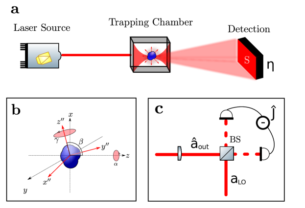
Figure 1: (a) An incoming coherent light beam creates an optical trap. A fraction of the photons is scattered, and a fraction of these is then recorded by the detector: the surface and efficiency of the detector are denoted by $S$ and $\eta$, respectively. (b) The laboratory axis are denoted by $x$, $y$, $z$ letters, while the body-frame axis are denoted by the $x^{\prime\prime}$, $y^{\prime\prime}$, $z^{\prime\prime}$ letters. The relation between the two frames is parametrized by the Euler angles $\alpha$, $\beta$ and $\gamma$ in z-y’-z” convention. $\alpha$ denotes the angle of rotation about the laboratory $z$ axis (from $x$ towards $y$). $\beta$ is the angle between the laboratory $z$ axis and the body $z^{\prime\prime}$ axis (rotated about the $y^{\prime}$ axis, i.e. the $y$ axis after it has been rotated by $\alpha$ about the $z$ axis; from $z$ towards $x$). $\gamma$ denotes the angle of rotation about the body frame $z^{\prime\prime}$ axis (from $x^{\prime\prime}$ towards $y^{\prime\prime}$). (c) Homodyne detection setup. $\hat{a}_{\text{out}}$ and $a_{\text{LO}}$ denote the signal (output operator), and the local oscillator (a complex number), respectively. These enter as inputs to the beam splitter, which we denote by BS. The outputs then get subtracted to obtain the measured photo-current $\hat{J}$ in the Heisenberg picture. We denote the corresponding photo-current in the Schrödinger picture by $J$ (see Sec. III.2).

We first discuss light-matter interactions. The incoming tightly focused light beam with a Gaussian profile creates an optical trap, which traps a nanoparticle near its focus point. This corresponds classically to the gradient force and torque. Moreover, the incoming light beam carries also linear and angular momentum. The linear momentum creates a radiation pressure scattering force which displaces the particle along the $z$ axis, while the angular momentum carried by the photons is transferred to the particle, which starts to rotate, i.e. spinning.

We next discuss collisions with the surrounding gas, which is a source of friction. Specifically, the gas of particles acts as a bath for the translational and rotational motions. In the simplest case we expect the particle to eventually reach an out of equilibrium steady state with the surrounding gas: the laser continuously transfers energy to the particle, which is then dissipated into the gas. This results in a specific variance of the translational and librational degrees of freedom, or, in the case of spinning, an asymptotic angular frequency.

Both photon scattering and gas collisions are a source of diffusion: each random collision, either with a photon or with a gas particle, makes the particle recoil. Loosely speaking, the net effect of these collisions is a stochastic trajectory of the particle state (monitoring by the environment with unit efficiency). In addition, the interaction with photons, as well as with gas particles, couples the rotational and translational motion: only in some limiting cases the motions decouple.

There is however an important difference between photon scattering and gas collisions. Suppose that the characteristic length of the optically levitated particle is $r_{s}$, denote the photon wavelength by $\lambda$, and the wavelength associated to a gas particle by $\lambda_{g}\approx\frac{2\pi\hbar}{\sqrt{2m_{g}k_{b}T}}$, where $T$ is the gas temperature, $m_{g}$ is the mass of a gas particle, and $k_{b}$ is Boltzman’s constant. For photon scattering we are in the long wavelength limit, while for gas collisions, for temperatures above $\sim 1\text{mK}$, we are in the short wavelength limit, i.e. $\lambda_{g}<r_{s}<\lambda$. Thus we will model the optically levitated particle in two different ways: on the one hand, for photon scattering, we can approximate it as an anisotropic particle with six degrees of freedom, while, on the other hand, for gas collisions, we will model it initially as a many-body system. However, under some simplifying assumption, e.g. rigid body, the latter will also reduce to the anisotropic particle model with six degrees of freedom.

II.2 Free Hamiltonian

We model the optically levitated system as an anisotropic polarizable particle with six degrees of freedom, i.e. three translational and three rotational. We denote the position and momentum operators by $\hat{\bm{r}}=(\hat{x},\hat{y},\hat{z})^{\top}$ and $\hat{\bm{p}}=(\hat{p}_{x},\hat{p}_{y},\hat{p}_{z})^{\top}$, respectively, the angle operator by $\hat{\mathbf{\mathbf{\mathbf{\boldsymbol{\phi}}}}}=(\hat{\alpha},\hat{\beta},\hat{\gamma}){}^{\top}$, where the three operators denote the quantized Euler angles in the $z$-$y^{\prime}$-$z^{\prime\prime}$ convention, and the corresponding (angle) momentum operator by $\hat{\bm{\pi}}=(\hat{\pi}_{\alpha},\hat{\pi}_{\beta},\hat{\pi}_{\gamma})^{\top}$.

We consider the free Hamiltonian for translational and rotational degrees of freedom:

$$\hat{H}_{\text{free}}=\frac{\hat{\bm{p}}^{\top}\hat{\bm{p}}}{2M}+\frac{\hat{\mathbf{\bm{\pi}}}^{\top}\hat{N}^{-1}\hat{F}I^{-1}\hat{F}^{\top}(\hat{N}^{\top}){}^{-1}\hat{\mathbf{\bm{\pi}}}}{2},$$ (1)

where $M$ is the mass of the system, $I=\text{diag}(I_{1},I_{2},I_{3})$ is the moment of inertia tensor in the principal axis (the body frame), $\hat{F}(\hat{\mathbf{\mathbf{\mathbf{\boldsymbol{\phi}}}}})=F_{\text{z}}(\hat{\alpha})F_{\text{y'}}(\hat{\beta})F_{\text{z''}}(\hat{\gamma})$ is the Euler parametrization of a generic rotation, $F_{x}$ denotes a rotation about the $x$-axis (here $x$ denotes a generic axis), and $\hat{N}(\hat{\mathbf{\mathbf{\mathbf{\boldsymbol{\phi}}}}})$ is the matrix that maps $\dot{\hat{\mathbf{\mathbf{\mathbf{\boldsymbol{\phi}}}}}}$ to the angular frequency $\hat{\boldsymbol{\omega}}$ in the laboratory frame, i.e. $\hat{\boldsymbol{\omega}}=\hat{N}(\hat{\boldsymbol{\mathbf{\mathbf{\mathbf{\phi}}}}})\dot{\hat{\mathbf{\boldsymbol{\phi}}}}$ (see Fig. 1(b)).

II.3 Light-matter coupling

The total electric field $\hat{\bm{E}}$ induces a dipole proportional to $\propto\hat{\chi}\hat{\bm{E}}$, where $\hat{\chi}$ is the susceptibility tensor of the trapped particle, and we suppose that this induced field is coupled with $\bm{\hat{E}}$ by the usual dielectric coupling, i.e. $\propto\hat{\bm{E}}^{\top}\hat{\chi}\hat{\bm{E}}$. Specifically, we start from the following interaction Hamiltonian:

$$\hat{H}_{\text{int}}=-\frac{1}{2}V\epsilon_{0}\hat{\bm{E}}^{\top}\hat{\chi}\hat{\bm{E}},$$ (2)

where $\hat{\bm{E}}(\hat{\bm{r}})$ is the total electric field, $\epsilon_{0}$ is the electric permittivity of free space, $\hat{\chi}=\hat{F}\chi\hat{F}^{\top}$, $\chi=\text{diag}(\chi_{1},\chi_{2},\chi_{3})$ is the electric susceptibility tensor in the body frame, and $V$ is the volume of the nanoparticle. We assume that $\chi_{j}$ are $\mathbb{R}$-valued, i.e. we consider only photon scattering, neglecting absorption and emission.

The total electric field is given by

$$\hat{\bm{E}}=\bm{\hat{E}}_{d}+\bm{\hat{E}}_{f}$$ (3)

where $\bm{\hat{E}}_{d}$ is the field that generates the optical trap and $\hat{\bm{E}}_{f}$ denotes the free electromagnetic field. Loosely speaking, one can think of a single incoming photon travelling in empty space (associated to the $\hat{\bf{E}}_{d}$ field), that at the nanoparticle location changes to an outgoing photon (associated to either the $\hat{\bf{E}}_{d}$ or the $\hat{\bf{E}}_{f}$ field). This way of separating the electrical field in two terms is reminiscent of the double counting of the output modes in cavity QED dutra2005cavity ; romero2011optically .

Specifically, we consider

$$\bm{\hat{E}}_{d}=iE_{0}(\mathbf{\boldsymbol{\mathbf{\bm{\epsilon}}}}_{d}\hat{u}\hat{a}-\boldsymbol{\mathbf{\bm{\epsilon}}}_{d}^{*}\hat{u}^{*}\hat{a}^{\dagger}),$$ (4)

where $E_{0}$ is the amplitude of the field, $\boldsymbol{\boldsymbol{\mathbf{\epsilon}}}_{d}$ is the polarization vector, $\hat{u}(\hat{\mathbf{r}})$ is the mode function, and $\hat{a}$ ($\hat{a}^{\dagger}$) the corresponding annihilation (creation) operator. Moreover, we will consider the case of elliptical polarization

$$\mathbf{\boldsymbol{\epsilon}}_{d}=\frac{1}{\sqrt{b_{x}^{2}+b_{y}^{2}}}(b_{x},ib_{y},0)^{\top},$$ (5)

where $b_{x}$, $b_{y}$ are $\mathbb{R}$-valued, and $\boldsymbol{\epsilon}_{d}^{*\top}\boldsymbol{\epsilon}_{d}=1$. More generally, in particular going beyond the paraxial approximation, one could consider also the case $\boldsymbol{\epsilon}_{d}=\boldsymbol{\epsilon}_{d}(\hat{\mathbf{r}})$.

The free electromagnetic field, which forms a bath, is given by:

$$\bm{\hat{E}}_{f}=i\sum_{\bm{k},\nu}\sqrt{\frac{\hbar\omega_{k}}{2V_{q}\epsilon_{0}}}\left(\bm{\epsilon}_{\bm{k},\nu}\hat{a}_{\bm{k},\nu}e^{i\bm{k}\cdot\hat{\bm{r}}}-\bm{\epsilon}_{\bm{k},\nu}^{*}\hat{a}_{\bm{k},\nu}^{\dagger}e^{-i\bm{k}\cdot\hat{\bm{r}}}\right)$$ (6)

where $\hat{a}_{\bm{k},\nu}$ ($\hat{a}_{\bm{k},\nu}^{\dagger}$) is the annihilation (creation) operator, $\bm{\epsilon}_{\bm{k},\nu}$ is the polarization vector, $\bm{k}$ is the wave-vector, $\nu$ denotes the two independent polarizations, $\omega_{k}=ck$, and $k=|\bm{k}|$. The quantization volume $V_{q}$ is determined the boundaries of the experimental setup walls2007quantum , e.g. $V_{q}=L^{3}$ with $L$ the size of a box. In case of a cavity system, the boundaries of the problem can be taken as the physical boundaries of the cavity, while for a system in free space the boundaries are at spatial infinity. This latter situation could also be applicable, in first approximation, to a system confined to a large or lossy cavity, i.e. whenever the field description given by Eq. (6) in the limit $V_{q}\rightarrow\infty$ is sufficient. In this paper, we restrict to this latter case of free space quantization, i.e. we consider the continuum limit by making the formal replacements $\sum_{\bm{k},\nu}\rightarrow\frac{V_{q}}{(2\pi)^{3}}\int d\bm{k}$ and ${\sqrt{V_{q}}}\hat{a}_{\bf{k},\nu}\rightarrow\hat{a}_{\bf{k},\nu}$. Note also that $\bm{\epsilon}_{\bm{k},\nu}=\bm{\epsilon}_{\bm{n},\nu}$ and $\bm{\epsilon}_{\bm{n},\nu}^{*\top}\bm{\epsilon}_{\bm{n},\nu}=1$, where $\bm{n}$ is a unit vector in the direction of $\bm{k}$, i.e. $\bm{k}=k\bm{n}$. For more details about the decomposition in Eq. (6) see Appendix A. In the following we will also use the completeness relation:

$$\sum_{\nu}(\bm{\epsilon}_{\bm{\bm{n}},\nu})_{i}(\bm{\epsilon}_{\bm{\bm{n}},\nu}^{*})_{j}=\delta_{ij}-\bm{n}_{i}\bm{n}_{j}.$$ (7)

We consider the usual Hamiltonian contribution of the free electromagnetic field:

$$H_{f}=\sum_{\nu}\int\frac{d\bm{k}}{(2\pi)^{3}}\hbar\omega_{k}\hat{a}_{\bm{k},\nu}^{\dagger}\hat{a}_{\bm{k},\nu}$$ (8)

We now use Eq. (3) in Eq. (2) from which we obtain two main contributions: the term $\propto\bm{\hat{E}}_{d}^{\top}\hat{\chi}\bm{\hat{E}}_{d}$, which gives rise to the unitary dynamics, and the term $\propto\bm{\hat{E}}_{f}^{\top}\hat{\chi}\bm{\hat{E}}_{d}$, which gives rise to the non-unitary dynamics, while we neglect $\propto\bm{\hat{E}}_{f}^{\top}\hat{\chi}\bm{\hat{E}}_{f}$, as we assume that the free-field modes are initially empty. Classically these correspond to the gradient and radiation pressure terms, respectively: we now discuss each of these separately.

II.3.1 Gradient terms

We consider the term $\propto\bm{\hat{E}}_{d}^{\top}\hat{\chi}\bm{\hat{E}}_{d}$, where $\bm{\hat{E}}_{d}$ is given in Eq. (4). Specifically, from Eqs. (2)-(5), making the rotating wave approximation (we take the time-average of optical fields, which we assume to oscillate much faster than the typical nanoparticle frequency), we obtain the gradient potential:

$$\hat{H}_{\text{grad}}=-\boldsymbol{\epsilon}_{0}VE_{0}^{2}|\hat{u}|^{2}(\mathbf{\boldsymbol{\mathbf{\epsilon}}}_{d}^{*})^{\top}\hat{\chi}\mathbf{\boldsymbol{\epsilon}}_{d}\hat{a}^{\dagger}\hat{a},$$ (9)

where

$$(\boldsymbol{\mathbf{\epsilon}}_{d}^{*})^{\top}\hat{\chi}\mathbf{\boldsymbol{\epsilon}}_{d} =b_{x}^{2}\bigg{[}\text{$\chi$}_{1}(\cos(\hat{\alpha})\cos(\hat{\beta})\cos(\hat{\gamma})-\sin(\hat{\alpha})\sin(\hat{\gamma}))^{2}$$

$$\;\;\;\;+\text{$\chi$}_{2}(\cos(\hat{\alpha})\cos(\hat{\beta})\sin(\hat{\gamma})+\sin(\hat{\alpha})\cos(\gamma))^{2}$$

$$\;\;\;\;+\text{$\chi$}_{3}\cos^{2}(\alpha)\sin^{2}(\beta)\bigg{]}$$

$$+b_{y}^{2}\bigg{[}\text{$\chi$}_{1}(\sin(\hat{\alpha})\cos(\hat{\beta})\cos(\hat{\gamma})+\cos(\hat{\alpha})\sin(\hat{\gamma}))^{2}$$

$$\;\;\;\;+\text{$\chi$}_{2}(\cos(\hat{\alpha})\cos(\hat{\gamma})-\sin(\hat{\alpha})\cos(\hat{\beta})\sin(\hat{\gamma}))^{2}$$

$$\;\;\;\;+\text{$\chi$}_{3}\sin^{2}(\hat{\alpha})\sin^{2}(\hat{\beta})\bigg{]}.$$ (10)

For $b_{x}=b_{y}$ we obtain circular polarization, while for $b_{x}=0$ or $b_{y}=0$ we obtain linear polarization along the $y$ or $x$ axis, respectively.

We now assume that the field $\bm{\hat{E}}_{d}$ is coherent and make the replacement $\hat{a}\rightarrow a$, where $a$ on the right hand-side denotes a $\mathbb{C}$-value, which simplifies Eq. (9) to the potential $\hat{H}_{\text{grad}}=-V\epsilon_{0}E_{0}^{2}|\hat{u}|^{2}|a|^{2}(\mathbf{\boldsymbol{\epsilon}}_{d}^{*})^{\top}\hat{\chi}\mathbf{\boldsymbol{\epsilon}}_{d}$. In a more refined analysis one should also consider the effect of quantum fluctuations of the incoming field, i.e. $\hat{a}=a+\delta\hat{a}$, where $\delta\hat{a}$ denote the quantum fluctuations. In particular, the $\delta\hat{a}$ contribution could lead to additional decoherence effects for the nanoparticle. We leave a more refined analysis, taking into account the quantum nature of the incoming optical field, for future research greiner1997classical .

We now want to express the gradient potential in terms of experimentally controllable parameters. To this end suppose that the transverse cross-section of the beam is given by $\sigma_{L}$. In this case we have that

$$\epsilon_{0}E_{0}^{2}|a|^{2}=\frac{P}{c\sigma_{L}},$$ (11)

where $P$ is the laser power, and $c$ is the speed of light. Using Eq. (11) we then immediately find $\hat{H}_{\text{grad}}=-\frac{VP}{c\sigma_{L}}|\hat{u}|^{2}(\mathbf{\boldsymbol{\epsilon}}_{d}^{*})^{\top}\hat{\chi}\mathbf{\boldsymbol{\epsilon}}_{d}$. One can then consider a generic expansion of $|u|^{2}$ up to a given order $\mathcal{O}((|\hat{\mathbf{r}}|/l)^{n})$:

$$\frac{VP}{c\sigma_{L}}|\hat{u}|^{2}=\sum_{k+l+m\leq n}c_{k,l,m}\hat{x}^{k}\hat{y}^{l}\hat{z}^{m},$$ (12)

where $n\in\mathbb{N}$, and $l$ has dimensions of length. In general we have $\frac{(n+2)(n+1)}{2}$ free parameters up to and including order $n$.

For example, one can consider a slightly modified Gaussian mode:

$$\hat{u}(\hat{r})=\frac{w_{0}}{w(\hat{z})}\text{exp}\left(-\frac{a_{1}\hat{x}^{2}+a_{2}\hat{y}^{2}}{w(\hat{z})^{2}}\right)e^{ik\hat{z}},$$ (13)

where $a_{1}$, $a_{2}$ are two adimensional parameters that quantify the asymmetry, $w(\hat{z})=w_{0}\sqrt{1+\left(\frac{\hat{z}}{z_{R}}\right)^{2}}$, $w_{0}$ is the beam waist, $k=\frac{2\pi}{\lambda}$, and $\lambda$ is the laser wavelength. In this case, assuming $w_{0}\sim\lambda$ and $z_{R}\sim\lambda$, the relevant length scale for the expansion in Eq. (12) is given b $l=\lambda$. The asymmetry between $\hat{x}$ and $\hat{y}$ could arise for example due to the use of elliptical polarization so2016tuning or simply due to misalignment of the optical elements. In Eq. (13) we have for concreteness considered a travelling wave ($e^{ik\hat{z}}$), but an experimental situation with a standing wave can be described in a similar fashion. When the particle is confined close to the center of the trap, i.e. $\frac{|\hat{x}|}{\lambda}$,$\frac{|\hat{y}|}{\lambda}$ and $\frac{|\hat{z}|}{\lambda}$ are small, then only the harmonic terms are manifest in the dynamics of the nanoparticle ($c_{2,0,0}\propto-\frac{2a_{1}}{w_{0}^{2}}$, $c_{0,2,0}\propto-\frac{2a_{2}}{w_{0}^{2}}$, and $c_{0,0,2}\propto-\frac{1}{z_{R}^{2}}$). On the other hand, if the nanoparticle starts exploring a larger region of the trap, then the first nonlinear terms start to become important, i.e. the quartic terms ($c_{4,0,0}\propto\frac{2a_{1}^{2}}{w_{0}^{4}}$, $c_{0,4,0}\propto\frac{2a_{2}^{2}}{w_{0}^{4}}$, and $c_{0,0,4}\propto\frac{1}{z_{R}^{4}}$), and the cross coupling terms ($c_{2,2,0}\propto\frac{4a_{1}a_{2}}{w_{0}^{4}}$, $c_{2,0,2}\propto\frac{4a_{1}}{w_{0}^{2}z_{R}^{2}}$, and $c_{0,2,2}\propto\frac{4a_{2}}{w_{0}^{2}z_{R}^{2}}$ ).

II.3.2 Scattering terms

We consider the term $\propto\bm{\hat{E}}_{f}^{\top}\hat{\chi}\bm{\hat{E}}_{d}$, where $\bm{\hat{E}}_{d}$ and $\bm{\hat{E}}_{f}$ are given in Eqs. (4) and (6), respectively (as discussed below Eq. (6) we consider the continuum limit, i.e. $V_{q}\rightarrow\infty$). This term, after tracing out the free field degrees of freedom gives a decoherence term agarwal2012quantum . Specifically, from Eqs. (2), (3) we obtain the interaction Hamiltonian

$$\hat{H}_{\text{scattering}}=\sum_{\nu,\mu}\int\frac{d\bm{k}}{(2\pi)^{3}}\hat{B}_{\bm{k},\nu,\mu}\hat{S}_{\bm{k},\nu,\mu},$$ (14)

where

$$\hat{B}_{\bm{k},\nu,\mu}=\begin{cases}\hat{a}_{\bm{k},\nu}\,,&\text{for}\,\mu=0,\\ \hat{a}_{\bm{k},\nu}^{\dagger}\,,&\text{for}\,\mu=1,\end{cases}$$ (15)

are the bath operators, and

$$\hat{S}_{\bm{k},\nu,\mu}=\begin{cases}-i\sqrt{\frac{\hbar\omega_{k}}{2\epsilon_{0}}}e^{i\bm{k}\cdot\hat{\bm{r}}}\bm{\epsilon}_{\bm{k},\nu}^{\top}(\epsilon_{0}V\hat{\chi}\bm{\hat{E}}_{d})\,,&\text{for}\,\mu=0,\\ i\sqrt{\frac{\hbar\omega_{k}}{2\epsilon_{0}}}e^{-i\bm{k}\cdot\hat{\bm{r}}}\bm{\epsilon}_{\bm{k},\nu}^{*\top}(\epsilon_{0}V\hat{\chi}\bm{\hat{E}}_{d})\,,&\text{for}\,\mu=1,\end{cases}$$ (16)

are the system operators. We assume a zero temperature bath (corresponding to an initially empty bath):

$$\langle\hat{a}_{\bm{k},\nu},\hat{a}_{\bm{k}^{\prime},\nu^{\prime}}\rangle =\langle\hat{a}_{\bm{k},\nu}^{\dagger},\hat{a}_{\bm{k}^{\prime},\nu^{\prime}}^{\dagger}\rangle=\langle\hat{a}_{\bm{k},\nu}^{\dagger},\hat{a}_{\bm{k}^{\prime},\nu^{\prime}}\rangle=0\,,$$ (17)

$$\langle\hat{a}_{\bm{k},\nu},\hat{a}_{\bm{k}^{\prime},\nu^{\prime}}^{\dagger}\rangle =\delta^{(3)}(\bm{k}-\bm{k}^{\prime})\delta_{\nu,\nu^{\prime}}\,.$$ (18)

The assumption of zero bath temperature can be understood by noting that the bath is associated to the scattered photons: before the event of scattering of an incoming photon takes place, the bath consists of unpopulated modes, i.e. there are no scattered photons. Once a photon is then scattered, it populates a particular mode of the bath, but under the assumption of no self interaction between the bath modes, the bath for the next scattered photon immediately resets to an empty bath. Loosely speaking, one can think that two consecutive scattered photons are distant in time such that it is possible to account for them individually, at least as far as the overall effect on the nanoparticle’s dynamics is concerned. Moreover, if the incoming field $\hat{\bm{E}}_{d}$, assumed classical, scatters into $\hat{\bm{E}}_{d}$, this do not lead to decoherence terms, but is already accounted for by the unitary gradient terms in Sec. II.3.1.

In the Born Markov approximation, assuming the particle degrees of freedom are not evolving during photon scattering (we assume that the incoming and scattered wavelengths are the same, i.e. Rayleigh scattering), making the rotating wave approximation (we time-average over the fast oscillations of the optical fields), supposing that the field $\hat{\bm{E}}{}_{d}$ is coherent (we make the replacement $\hat{a}\rightarrow a$, where $a$ on the right hand-side denotes a $\mathbb{C}$-value), using Eq. (11) and Eqs. (14)-(18), we eventually obtain the Lindblad dissipator:

$$\mathcal{L}_{\text{scattering}}[\,\cdot\,]= \gamma_{s}\sum_{\nu}\int d\bm{n}\bigg{(}\hat{A}_{\bm{n},\nu}\,\cdot\,\hat{A}_{\bm{n},\nu}^{\dagger}$$

$$-\frac{1}{2}\left\{\hat{A}_{\bm{n},\nu}^{\dagger}\hat{A}_{\bm{n},\nu},\,\cdot\,\right\}\bigg{)},$$ (19)

where

$$\hat{A}_{\bm{n},\nu}=(\bm{\epsilon}_{k\bm{n},\nu}^{*\top}\hat{\chi}\bm{\epsilon}_{d})\hat{u}e^{i\bm{k}\cdot\hat{\bm{r}}},$$ (20)

and

$$\gamma_{s}=\frac{\tilde{\sigma}_{R}}{\sigma_{L}}\frac{P}{\hbar\omega_{L}}$$ (21)

is the scattering rate. $\bm{n}$ denotes the unit vector and $\tilde{\sigma}_{R}=\frac{\pi^{2}V_{0}^{2}}{\lambda^{4}}$ is an effective cross-section area. For the case of an isotropic polarizable point particle, Eq. (19) reduces to the dissipator considered in nimmrichter2014macroscopic ; rashid2017wigner : in particular, we also re-obtain the Rayleigh cross-section $\sigma_{R}=\frac{24\pi^{3}V_{0}^{2}}{\lambda^{4}}\left(\frac{\epsilon_{R}-1}{\epsilon_{R}+2}\right)^{2}$, where $\epsilon_{R}$ is the dielectric function, by combing the factors contained in $\tilde{\sigma}_{R}$ and $\chi$. The case of linear rotors with linearly polarized light, and the case of arbitrary rotors with unpolarized light has been discussed in stickler2016rotranslational ; stickler2016spatio and papendell2017quantum , respectively.

II.4 Gas collisions

To account for the interaction with the gas of particles we suppose that the optically levitated particle is a many-body rigid system composed of $n$ particles. Specifically, we model the effect of gas collisions on this system using the dissipative Caldeira-Leggett master equation caldeira1985physica ; breuer2002theory :

$$\mathcal{L}_{\text{collisional}}[\,\hat{\rho}\,]=\frac{i\gamma_{c}}{2\hbar}\sum_{j=1}^{n}\left[\hat{\boldsymbol{r}}_{n}\cdot\hat{\boldsymbol{p}}_{n}+(\hat{\boldsymbol{r}}_{n}\cdot\hat{\boldsymbol{p}}_{n})^{\dagger},\hat{\rho}\right]$$

$$\quad+\frac{4mk_{b}T\gamma_{c}}{\hbar^{2}}\sum_{j=1}^{n}\left(\hat{\tilde{\boldsymbol{L}}}_{n}\cdot\rho\hat{\tilde{\boldsymbol{L}}}_{n}^{\dagger}-\frac{1}{2}\left\{\hat{\tilde{\boldsymbol{L}}}_{n}\cdot\hat{\tilde{\boldsymbol{L}}}_{n}^{\dagger},\hat{\rho}\right\}\right)$$ (22)

where $\hat{\boldsymbol{r}}_{n}$ and $\hat{\boldsymbol{p}}_{n}$ are the position and momentum operators of particle $n$, respectively, $m$ is the mass of a single particle, $\gamma_{c}$ is the collision rate (assumed for simplicity the same for each particle), $k_{b}$ is Boltzman constant, $T$ is the temperature of the gas, and

$$\hat{\tilde{\boldsymbol{L}}}_{n}=\hat{\boldsymbol{r}}_{n}+\frac{i\hbar}{4mk_{b}T}\hat{\boldsymbol{p}}_{n}$$ (23)

We now change to the center-of-mass (c.m.) coordinates:

$$\hat{\boldsymbol{r}}_{j} =\hat{\boldsymbol{r}}+\hat{\tilde{\boldsymbol{r}}}_{j},$$ (24)

$$\hat{\boldsymbol{p}}_{j} =\frac{m}{M}\hat{\boldsymbol{p}}+\hat{\tilde{\boldsymbol{p}}}_{j},$$ (25)

where $\hat{\boldsymbol{r}}$, $\hat{\boldsymbol{p}}$, $\hat{\tilde{\boldsymbol{r}}}_{n}$, $\hat{\tilde{\boldsymbol{p}}}_{n}$ are the c.m. position, c.m. momentum, relative position of $n$-th particle, relative momentum of $n$-th particle, operators, respectively, and $M=nm$ is the total mass. We now use Eqs. (24), (25), and the relations $\sum_{j=1}^{n}\hat{\tilde{\boldsymbol{r}}}_{j}=0$, $\sum_{j=1}^{n}\hat{\tilde{\boldsymbol{p}}}_{j}=0$, to decouple c.m. and relative degrees of freedom in Eq. (22):

$$\mathcal{L}_{\text{collisional}}[\,\cdot\,]=\mathcal{L}_{\text{collisional}}^{(t)}[\,\cdot\,]+\mathcal{L}_{\text{collisional}}^{(r)}[\,\cdot\,],$$ (26)

where $\mathcal{L}_{\text{collisional}}^{(t)}[\,\cdot\,]$ and $\mathcal{L}_{\text{collisional}}^{(r)}[\,\cdot\,]$ denote the dissipator on translations and, as discussed below, rotations, respectively. Specifically, we find the following dissipator for translations:

$$\mathcal{L}_{\text{collisional}}^{(t)}[\,\hat{\rho}\,]=\frac{i\gamma_{c}}{2\hbar}\left[\hat{\boldsymbol{r}}\cdot\hat{\boldsymbol{p}}+(\hat{\boldsymbol{r}}\cdot\hat{\boldsymbol{p}})^{\dagger},\hat{\rho}\right]$$

$$\quad+\frac{4Mk_{b}T}{\hbar^{2}}\gamma_{c}\left(\hat{\tilde{\boldsymbol{L}}}\cdot\rho\hat{\tilde{\boldsymbol{L}}}^{\dagger}-\frac{1}{2}\left\{\hat{\tilde{\boldsymbol{L}}}\cdot\hat{\tilde{\boldsymbol{L}}}^{\dagger},\hat{\rho}\right\}\right),$$ (27)

where $\hat{\tilde{\boldsymbol{L}}}=\hat{\boldsymbol{r}}+\frac{i\hbar}{4Mk_{b}T}\hat{\boldsymbol{p}}$. Under the assumption of a rigid body we eventually find the following dissipator for rotations:

$$\mathcal{L}_{\text{collisional}}^{(r)}[\,\hat{\rho}\,]= \frac{4mk_{b}T}{\hbar^{2}}\gamma_{c}\sum_{\zeta=1}^{3}\tilde{D}_{\zeta}\bigg{(}\left[\hat{\tilde{\boldsymbol{C}}}_{\zeta}\cdot\hat{\rho}\hat{\tilde{\boldsymbol{C}}}_{\zeta}^{\dagger}\right]$$

$$-\frac{1}{2}\left\{\hat{\tilde{\boldsymbol{C}}}_{\zeta}^{\dagger}\cdot\hat{\tilde{\boldsymbol{C}}}_{\zeta},\hat{\rho}\right\}\bigg{)},$$ (28)

where

$$\hat{\tilde{\boldsymbol{C}}}_{\zeta}=\hat{F}\mathbf{e}_{\zeta}-\frac{i\hbar}{4k_{b}T}\hat{F}L_{\zeta}I^{-1}\hat{F}^{\top}(\hat{N}^{\top})^{-1}\hat{\bm{\pi}},$$ (29)

$\boldsymbol{e}_{\zeta}$ is the unit vector along the $\zeta$-axis, $L_{\zeta}$ is the generator of rotations about the $\zeta$-axis, and

$$\tilde{D}_{\zeta}=(\frac{1}{2}\text{tr}I-I_{\zeta}).$$ (30)

The moment of inertia tensor $I$, the Euler parametrization $\hat{F}$ of a generic rotation, and the matrix $\hat{N}$ have been defined in Sec. II.2. For later convenience, we also define the operators:

$$\hat{L}_{j} =\frac{i\sqrt{4Mk_{b}T}}{\hbar}\hat{\tilde{\boldsymbol{L}}}\cdot\boldsymbol{e}_{j},$$ (31)

$$\hat{\boldsymbol{C}}_{\zeta,j} =\frac{i\sqrt{4k_{b}T\tilde{D}_{\zeta}}}{\hbar}\hat{\tilde{\boldsymbol{C}}}_{\zeta}\cdot\boldsymbol{e}_{j}.$$ (32)

The case of rotational diffusion without friction is discussed in papendell2017quantum , while the dissipator in Eq. (28) has been derived in stickler2017rotational .

II.5 Non-inertial terms

For completeness we also include the non-inertial term, which arises in Earth-bound laboratories. Specifically, we consider the following contribution to the Hamiltonian:

$$\hat{H}_{\text{ni}}=Mg\hat{x},$$ (33)

where $M$ is the total mass, and $g$ is the gravitational acceleration. Although the contribution from this term is typically much smaller than from light-matter interactions and gas collisions, it can become relevant in certain experimental settings kuhn2015cavity ; hebestreit2017sensing ; stickler2018orientational .

III Detection for ro-translation

In this section we combine the terms from the previous Sec. II and discuss the resulting dynamics. In particular, we consider the unconditional dynamics, i.e. without a detector keeping track of the intensity gathered from the collected scattered photons, and the dynamics conditioned upon the measured intensity in a general dyne detection. We then apply the obtained formulae to construct to a toy model of homodyne detection.

III.1 Dyne detection

The dynamics of the optically levitated particle is given by:

$$\dot{\hat{\rho}}= -\frac{i}{\hbar}[\hat{H}_{\text{free}}+\hat{H}_{\text{gradient}}+\hat{H}_{\text{ni}},\hat{\rho}]$$

$$+\mathcal{L}_{\text{scattering}}[\hat{\rho}]+\mathcal{L}_{\text{collisional}}[\hat{\rho}]$$ (34)

where $\hat{H}_{\text{free}}$, $\hat{H}_{\text{grad}}$, $\mathcal{L}_{\text{scattering}}[\,\cdot\,]$, and $\mathcal{L}_{\text{collisional}}[\,\cdot\,]$ are defined in Eqs. (1), (9), (19), and (26), respectively, and $\hat{H}_{\text{ni}}$ is given in Eq. (33). We will refer to Eq. (1) as the unconditional dynamics, and to the state $\hat{\rho}$ as the unconditional state.

However, usually one collects part of the scattered light to update the knowledge about the state of the system. Here we consider the case when the scattered light interfers with a classical local oscillator before detection, namely, dyne detection (see Fig. 1(c)). A simple example of this type of approach is given by homodyne detection rashid2017wigner .

The detected photo-current (signal) allows to continuously update the description of the system: we will refer to the resulting state $\hat{\rho}_{c}$ as the conditional state. Mathematically we can describe this by considering an unraveling of the photon scattering term $\mathcal{L}_{\text{scattering}}[\hat{\rho}]$ in Eq. (34). The most general diffusive unraveling, also known as the Belavkin equation, is given by (in Itô form) wiseman2001complete ; WISEMAN2001227 :

$$d\hat{\rho}_{c}= \gamma_{s}\sum_{\nu=1}^{2}\int d\bm{n}\mathcal{D}[\hat{A}_{\bm{n},\nu}]\hat{\rho}_{c}dt$$

$$+\sqrt{\gamma_{s}}\sum_{\nu=1}^{2}\int d\bm{n}\mathcal{H}[\hat{A}_{\bm{n},\nu}dW_{\bm{n},\nu}^{*}]\hat{\rho}_{c},$$ (35)

where PhysRevA.47.1652

$$\mathcal{D}[\hat{K}]\,\cdot\, =\hat{K}\,\cdot\,\hat{K}^{\dagger}-\frac{1}{2}\left\{\hat{K}^{\dagger}\hat{K},\,\cdot\,\right\},$$ (36)

$$\mathcal{H}[\hat{K}]\,\cdot\, =\hat{K}\,\cdot\,+\,\cdot\,\hat{K}^{\dagger}-\text{tr}[\hat{K}\,\cdot\,+\,\cdot\,\hat{K}^{\dagger}]\,\cdot\,,$$ (37)

and $\hat{K}$ denotes an operator. Note that the first term on the right hand-side of Eq. (35) corresponds to $\mathcal{L}_{\text{scattering}}[\hat{\rho}]$ . $W_{\bm{n},\nu}$ are $\mathbb{C}$-valued, zero mean Wiener processes with correlations:

$$\mathbb{E}[dW_{\bm{n},\nu}dW_{\bm{n}^{\prime},\nu^{\prime}}^{*}] =dt\eta_{(\bm{n},\nu),(\bm{n}^{\prime},\nu^{\prime})},$$ (38)

$$\mathbb{E}[dW_{\bm{n},\nu}dW_{\bm{n}^{\prime},\nu^{\prime}}] =dt\varXi_{(\bm{n},\nu),(\bm{n}^{\prime},\nu^{\prime})}\,,$$ (39)

where the only non-zero elements of $\eta$ are $\eta_{(\bm{n},\nu),(\bm{n},\nu)}\in[0,1]$, $\varXi$ has $\mathbb{C}$-valued entries, $\varXi_{(\bm{n},\nu),(\bm{n}^{\prime},\nu^{\prime})}=\varXi_{(\bm{n}^{\prime},\nu^{\prime}),(\bm{n},\nu)}$, and

$$\frac{1}{2}\left(\begin{array}[]{cc}\eta+\mathbb{\text{Re}}(\varXi)&\mathbb{\text{Im}}(\varXi)\\ \mathbb{\text{Im}}(\varXi)&\eta-\mathbb{\text{Re}}(\varXi)\end{array}\right)$$ (40)

is positive semi-definite. The photo-currents associated to Eq. (35) are given by:

$$J_{\bm{n},\nu}dt= \text{tr}\bigg{[}\sum_{\nu^{\prime}=1}^{2}\int d\bm{n}^{\prime}\bigg{(}\eta_{(\bm{n},\nu),(\bm{n}^{\prime},\nu^{\prime})}\hat{A}_{\bm{n}^{\prime},\nu^{\prime}}$$

$$+\varXi_{(\bm{n},\nu),(\bm{n}^{\prime},\nu^{\prime})}\hat{A}_{\bm{n}^{\prime},\nu^{\prime}}^{\dagger}\bigg{)}\hat{\rho}_{c}\bigg{]}dt+dW_{\bm{n},\nu}.$$ (41)

Eqs. (35) and (41) is the conventional way of presenting the conditional dynamics: the stochastic nature of the dynamics and of the photo-current is explicit, where the stochasticity is due to the weak (imprecise) measurements of the system. However, one can also combine Eqs. (35) and (41) in a single equation that explicitly shows the dependency of the conditional dynamics on the measured photo-currents $J_{\bm{n},\nu}$. In particular, one can invert Eq. (41) to obtain the expression of $dW_{\bm{n},\nu}$ as a function of the measured photo-currents $J_{\bm{n},\nu}$, i.e. $dW_{\bm{n},\nu}(J_{\bm{n},\nu})$, which can be used to eliminate the Wiener processes $dW^{*}_{\bm{n},\nu}$ from Eq. (35):

$$d\hat{\rho}_{c}= \gamma_{s}\sum_{\nu=1}^{2}\int d\bm{n}\mathcal{D}[\hat{A}_{\bm{n},\nu}]\hat{\rho}_{c}dt$$

$$+\sqrt{\gamma_{s}}\sum_{\nu=1}^{2}\int d\bm{n}\mathcal{H}[\hat{A}_{\bm{n},\nu}dW_{\bm{n},\nu}(J_{\bm{n},\nu})^{*}]\hat{\rho}_{c},$$ (42)

The evolution of the conditional state $\hat{\rho}_{c}$ in Eq. (42) now explicitly depends on the currents $J_{\bm{n},\nu}$, which are inputs of the equation of motion. The conditional dynamics in Eq. (42) can be readily used for tracking or simulating the conditional state of the system setter2017real ; ralph2017dynamical .

The full conditional dynamics can be obtained by adding the Hamiltonian terms ($\hat{H}_{\text{free}}$, $\hat{H}_{\text{grad}}$ and $\hat{H}_{\text{ni}}$) and the non-unitary contribution from gas collisions ($\mathcal{L}_{\text{collisional}}$) to the right hand-side of Eqs. (35) or (42). Discontinuous unravellings, where each photon triggers a discontinuous update of the conditional state, could be treated in a similar way.

In general, the currents $J_{\bm{n},\nu}$ are $\mathbb{C}$-valued and thus cannot be directly associated to the intensity current measured by a physical detector: these can be reconstructed from the $\mathbb{R}$-valued currents $\text{Re}(J_{\bm{n},\nu})$ and $\text{Im}(J_{\bm{n},\nu})$, e.g. see heterodyne detection in wiseman2009quantum . In the next section we consider the case of homodyne detection, which is a special case of the formalism used in this section, where we obtain explicit expression for the physical photo-currents.

III.2 Homodyne detection model

In order to discuss a detection model we have to specify the measuring operator(s). In general, the measuring operator will be a functional of the system degrees of freedom as well as of the experimental setting, i.e. $\mathcal{A}[\hat{\boldsymbol{r}},\hat{\boldsymbol{\phi}};\text{exp.setting}]$. For example, only some of the scattered photons are collected by optical elements: these are then recorded by a physical detector, where the detector’s efficiency, orientation, distance, size, and integration time, all affect the measured signal. Here we consider a simplified detector model, completely characterized by the operator $\sqrt{\eta\gamma_{s}}\sum_{\nu=1}^{2}\int_{S}d\bm{n}\hat{A}_{\bm{n},\nu},$ where $S$ denotes the surface of a toy detector, $\gamma_{s}$ is defined in Eq. (21), and $\eta$ is the detector’s efficiency, i.e. we are considering the case when the efficiency matrix $\eta$ introduced in Sec. III.1 is proportional to the identity matrix, and completely characterized by a single number, which we also label as $\eta\in[0,1]$ (see Fig. 1(a)). In this case, as we show below, the total photo-current is of the form $\sum_{\nu}\int_{S}d\bm{n}\,J_{\boldsymbol{n},\nu}$, where $J_{\boldsymbol{n},\nu}$ is associated to $\hat{A}_{\bm{n},\nu}$.

This total photo-current, which we label as $J$, can be considered as a toy model for the experimental configuration in rashid2017wigner . Loosely speaking, optical elements, such as a paraboloidal mirror, collect the scattered photons and direct them towards the beam splitter: this conceals, at least partially, the information about the scattering direction $\boldsymbol{n}$ and polarization $\nu$. We denote the annihilation operator for the corresponding collective mode by $\hat{a}_{\text{out}}$, i.e. the annihilation operator of all the photons travelling towards the detector. At the beam splitter the signal from the scattered photons is combined with the local oscillator $a_{\text{LO}}$ (a $\mathbb{C}$-value) from which we obtain the current $J$ (see Fig. 1(c)). Here we are supposing that the local oscillators $\left(a_{\bm{n},\nu}\right)_{\text{LO}}$, for each direction $\bm{n}$ and polarization $\nu$, can be approximated by a single local oscillator $a_{\text{LO}}$. To obtain a more refined model of detection in this specific experimental situation, or to adapt it to describe a different experimental setup, one would need to take into account the specific details of the experiment and repeat the analysis, e.g. by imposing the specific boundary conditions.

We can now apply the general procedure discussed in the previous Sec. III.1. Specifically, for each dissipator term $D[\hat{A}_{\bm{n},\nu}]$ we have to consider the corresponding noise term $\mathcal{H}[\hat{A}_{\bm{n},\nu}dW_{\bm{n},\nu}]$, where we assume that $W_{\bm{n},\nu}$ are $\mathbb{R}$-valued and independent, since they are associated to different modes. As already mentioned above, we also suppose that each mode is detected with the same efficiency $\eta\in[0,1]$, which simplifies Eqs. (38) and (39) to

$$\mathbb{E}[dW_{\bm{n},\nu}dW_{\bm{n}^{\prime},\nu^{\prime}}]=\eta dt\delta_{\nu,\nu^{\prime}}\delta^{(2)}(\bm{n}-\bm{n}^{\prime}).$$ (43)

It is then straightforward to obtain the equation for the conditional state (in Itô form):

$$d\hat{\rho}_{c}= -\frac{i}{\hbar}[\hat{H}_{\text{free}}+\hat{H}_{\text{gradient}}+\hat{H}_{\text{ni}},\hat{\rho}_{c}]dt$$

$$+\gamma_{c}\sum_{j=1}^{3}\mathcal{D}[\hat{L}_{j}]\hat{\rho}_{c}dt+\gamma_{c}\sum_{\zeta,j=1}^{3}\mathcal{D}[\hat{\boldsymbol{C}}_{\zeta,j}]\hat{\rho}_{c}dt$$

$$+\gamma_{s}\sum_{\nu=1}^{2}\int d\bm{n}\mathcal{D}[\hat{A}_{\bm{n},\nu}]\hat{\rho}_{c}dt$$

$$+\sqrt{\gamma_{s}}\mathcal{H}[\sum_{\nu=1}^{2}\int_{S}d\bm{n}\hat{A}_{\bm{n},\nu}]\hat{\rho}_{c}dW.$$ (44)

$W$ is a zero mean, $\mathbb{R}$-valued Wiener process with correlation

$$\mathbb{E}[dWdW]=2\Omega\eta dt,$$ (45)

where $\Omega=\int_{S}d\bm{n}$, and the factor $2$ reflects the fact that both independent polarizations are detected. Using Eq. (41), summing all the currents, we finally obtain that the state $\hat{\rho}_{c}$ in Eq. (44) is conditioned on the following photo-current:

$$Jdt=\eta\sqrt{\gamma_{s}}\text{Tr}\left[\sum_{\nu=1}^{2}\int_{S}d\bm{n}\left(\hat{A}_{\bm{n},\nu}+\hat{A}_{\bm{n},\nu}^{\dagger}\right)\hat{\rho}_{c}\right]dt+dW.$$ (46)

We recover Eq. (34) from Eq. (44) by taking the expectation value $\mathbb{E}[\,\cdot\,]$ over the noise realizations. In case $dW$ is obtained from $J$ by inverting Eq. (46) one has to repeat the experiment or simulation to build enough statistics for J in order to recover Eq. (34).

III.2.1 Heisenberg picture

The above derivation in the Schrödinger picture, on the one hand, has the advantage that it clearly shows the effect of photon detection on the nanoparticle, i.e. one inverts Eq. (46) and then inserts the expression for $dW(J)$ in Eq. (44), on the other hand, it does not provide an intuitive picture of the interaction between the photons and the nanoparticle. This becomes more apparent in Heisenberg picture using the input-output formalism gardiner1985input ; gardiner2004quantum ; wiseman2009quantum . In a nusthell, an incoming photon $\hat{a}$, associated to the field $\hat{\bm{E}}_{d}$ interacts with the nanoparticle, which generates a signature in the scattered photon $\hat{a}_{\bm{n},\nu}$ associated to the field $\hat{\bm{E}}_{f}$. In particular, one labels the operator of the scattered photon, before and after the event of scattering takes place, as the input operator $\left(\hat{a}_{\bm{n},\nu}\right)_{\text{in}}$ and output operator $\left(\hat{a}_{\bm{n},\nu}\right)_{\text{out}}$, respectively. As the particle scatters the incoming photon, the input operator transforms to the output operator according to the following relation:

$$\left(\hat{a}_{\bm{n},\nu}\right)_{\text{out}}=\left(\hat{a}_{\bm{n},\nu}\right)_{\text{in}}+\sqrt{\gamma_{s}}\hat{A}_{\bm{n},\nu}\,,$$ (47)

The modelling of inefficient detection is slightly more involved in the Heisenberg picture. To show the close analogy with the Schrödinger picture analysis it is convenient to define the input quantum noise operator $d\hat{a}_{\text{in}}=\sum_{\nu=1}^{2}\int d\bm{n}\left(\hat{a}_{\bm{n},\nu}\right)_{\text{in}}dt$, where we have $[d\hat{a}_{\text{in}},d\hat{a}_{\text{in}}^{\dagger}]=2\Omega dt$, and to introduce a second auxiliary quantum noise operator $d\hat{v}$, such that $[d\hat{v},d\hat{v}^{\dagger}]=2\Omega dt$. Here we assume that the quantum noise operators act on the vacuum state of their corresponding bath. Loosely speaking we can think of $d\hat{a}_{\text{in}}$ as the quantum noise in case of a completely efficient detection, i.e. $\eta=1$, which starts to become completely dominated by the noise $d\hat{v}$ at low efficiencies, i.e. $\eta\ll 1$. This can be seen mathematically by formally introducing a new quantum noise operator $d\hat{w}$:

$$d\hat{w}=\eta\left(d\hat{a}_{\text{in}}+d\hat{a}_{\text{in}}^{\dagger}\right)+\sqrt{\eta(1-\eta)}\left(d\hat{v}+d\hat{v}^{\dagger}\right),$$ (48)

such that $\langle d\hat{w}\rangle=0$ and $\langle d\hat{w}d\hat{w}\rangle=2\Omega\eta dt$. The statistics of the photo-current $J$ in Eq. (46) can then be recovered by considering its Heisenberg picture equivalent (see Fig. 1(c)):

$$\hat{J}dt= \eta\sqrt{\gamma_{s}}\sum_{\nu}\int_{S}d\bm{n}\left((\hat{A}_{\bm{n},\nu}+\hat{A}_{\bm{n},\nu}^{\dagger}\right)dt+d\hat{w}.$$ (49)

In particular, one can readily show that

$$\mathbb{E}[J]=\langle\hat{J}\rangle,\qquad\mathbb{E}[(J-\mathbb{E}[J])^{2}]=\langle(\hat{J}-\langle\hat{J}\rangle)^{2}\rangle,$$ (50)

where $\mathbb{E}[\;\cdot\;]$ denotes the stochastic expectation value with respect to different noise realizations, and $\langle\;\cdot\;\rangle$ denotes the quantum trace operation with respect to the nanoparticle state and the vacuum states of the two baths. For more details see gardiner2004quantum ; wiseman2009quantum ; jacobs2014quantum .

III.2.2 Classical currents

It is useful to derive approximate photo-currents for a classical nanoparticle, e.g. for force and torque sensing applications. To this end we replace quantum observables $\hat{O}$ by their corresponding classical observables $O^{\text{(cl)}}$, and the commutators with Poisson Brackets, i.e $[\,\cdot\,,\,\cdot\,]\rightarrow i\hbar\{\,\cdot\,,\,\cdot\,\}_{\text{Pb}}$. In particular, following this procedure, we obtain from Eq. (46):

$$Jdt=2\eta\sqrt{\gamma_{s}}\sum_{\nu=1}^{2}\int_{S}d\bm{n}\text{Re}\left(A_{\bm{n},\nu}^{\text{(cl)}}e^{i\Delta\Phi}\right)dt+dW.$$ (51)

where we have introduced the phase $\Delta\Phi$ of the local oscillator. From Eq. (20) we also readily obtain the classical scattering observable:

$$A_{\bm{n},\nu}^{(cl)}(\bm{r},\bm{\phi})=[\bm{\epsilon}_{k\bm{n},\nu}^{*\top}F(\bm{\phi})\chi F(\bm{\phi})^{\top}\bm{\epsilon}_{d}]u(\bm{r})e^{i\bm{k}\cdot\bm{r}}.$$ (52)

Let us now consider separately the position and angle depended factors in $A_{\bm{n},\nu}^{\text{(cl)}}$. We assume the modified Gaussian mode in Eq. (13) and suppose that $\frac{|\boldsymbol{r}|}{\lambda}$ is small. In particular, we consider the expansion up to order $\mathcal{O}(|\boldsymbol{r}|^{2})$:

$$u(\bm{r})e^{i\bm{k}\cdot\bm{r}}\approx 1+i(k\bm{n}\bm{r}+kz)-k^{2}{\bm{n}}\cdot{\bm{r}}z-\frac{1}{2}k^{2}(\bm{n}\cdot\bm{r})^{2}$$

$$-\frac{a_{1}}{w_{0}^{2}}x^{2}-\frac{a_{2}}{w_{0}^{2}}y^{2}-\frac{z_{R}^{2}k^{2}+2}{2z_{R}^{2}}z^{2}$$ (53)

We also decompose the susceptibility tensor $\chi$ (in the body frame) in the following form:

$$\chi=\chi_{0}(\mathcal{I}+\Delta\chi)$$ (54)

where $\chi_{0}$ is the susceptibility in the limit of an isotropic particle, $\Delta\chi$ quantifies the degree of anisotropy, and $\mathcal{I}$ denotes the $3\times 3$ identity matrix. Using Eqs. (52)-(54) we can then decompose the expectation value of the photo-current in Eq. (51) in four parts:

$$\mathbb{E}[J(\bm{r},\bm{\phi};\Delta\Phi)]=J_{\text{0}}+J_{\text{T}}(\bm{r})+J_{\text{R}}(\bm{\phi})+J_{\text{RT}}(\bm{r},\bm{\phi}),$$ (55)

where $J_{\text{0}}$, $J_{\text{T}}$, $J_{\text{R}}$, and $J_{\text{RT}}$ denote a constant, a purely translational, a purely rotational, and the mixed ro-translational expectation values of the currents, respectively.

We first discuss the limit of an isotropic particle ($\Delta\chi\rightarrow 0$) such that the only non-trivial term in Eq. (55) is given by:

$$J_{\text{T}}(\bm{r};\Delta\Phi)= 2\eta\chi_{0}\sqrt{\gamma_{s}}\int_{S}d\bm{n}\text{Re}\bigg{[}\sum_{\nu=1}^{2}\bm{\epsilon}_{k\bm{n},\nu}^{*\top}\bm{\epsilon}_{d}e^{i\Delta\Phi}$$

$$\big{(}ik(\bm{n}\bm{r}+z)-k^{2}{\bm{n}}\cdot{\bm{r}}z-\frac{1}{2}k^{2}(\bm{n}\cdot\bm{r})^{2}$$

$$-\frac{a_{1}}{w_{0}^{2}}x^{2}-\frac{a_{2}}{w_{0}^{2}}y^{2}-\frac{z_{R}^{2}k^{2}+2}{2z_{R}^{2}}z^{2}\big{)}\bigg{]}.$$ (56)

In case of linearly polarized light $\bm{\epsilon}_{d}$ has $\mathbb{R}$-valued components and thus also $\sum_{\nu=1}^{2}\bm{\epsilon}_{k\bm{n},\nu}^{*\top}\bm{\epsilon}_{d}$ becomes $\mathbb{R}$-valued. By controlling the phase $\Delta\Phi$ of the local oscillator we can then decide to detect the position of the particle, i.e. the first term ($\propto\bm{n}\bm{r}+z$) on the second line of Eq. (56), or the squared value of position and cross-coupling terms, i.e. the last two terms on the second line and the last line of Eq. (56).

We next discuss the limit of small position oscillations ($|\bm{r}|\rightarrow 0$) such that the only non-trivial term in Eq. (55) is given by:

$$J_{\text{R}}({\bm{\phi}};\Delta\Phi)= 2\eta\chi_{0}\sqrt{\gamma_{s}}\int_{S}d\bm{n}\text{Re}\bigg{[}$$

$$\sum_{\nu=1}^{2}\bm{\epsilon}_{k\bm{n},\nu}^{*\top}F(\mathbf{\mathbf{\mathbf{\boldsymbol{\phi}}}})\Delta\chi F(\mathbf{\mathbf{\mathbf{\boldsymbol{\phi}}}})^{\top}\bm{\epsilon}_{d}e^{i\Delta\Phi}\bigg{]}.$$ (57)

If we consider again linearly polarized light, i.e. $\sum_{\nu=1}^{2}\bm{\epsilon}_{k\bm{n},\nu}^{*\top}\bm{\epsilon}_{d}$ is $\mathbb{R}$-valued, then we see that $\Delta\Phi$ controls the amplitude of the photocurrent $J_{\text{R}}$, but not the measured observable. This is in different from the translational current $J_{\text{T}}$ in Eq. (56), where the phase $\Delta\Phi$ of the local oscillator controls the amplitude as well as the measured observable.

The correction current $J_{\text{RT}}({\bm{r}},{\bm{\phi}};\Delta\Phi)$ can be obtained by combing $J_{\text{T}}({\bm{r}};\Delta\Phi)$ together with $J_{\text{R}}({\bm{\phi}};\Delta\Phi)$: specifically, $J_{\text{RT}}$ can be formally obtained by inserting the terms on the second and third lines of Eqs. (56) inside the square brackets of Eq. (57).

The formulae in Eqs. (56) and (57) can be used for investigating the conversion between the measured homodyne current $J$ and the nanoparticle position ($\bm{r}$) and orientation ($\bm{\phi}$). To include explicitly the amplitude of the local oscillator one can follow the approach taken in rashid2017wigner , which can be readily extended to include ro-translations. Moreover, while in this section we have discussed currents based on the measurement of classical observables, the same analysis can be applied also for the current based on quantum observables of the quantum model discussed in the previous sections. In particular, one obtains an analogous separation of the currents in translational, rotational, and ro-translational terms, as discussed below Eq. (55).

IV Summary

We have discussed the motion and detection of optically levitated nanoparticles. Specifically, we have considered an anisotropic particle trapped in an elliptically polarized Gaussian beam, and immersed in a bath of gas particles. We have first introduced the dynamics of such systems using notions of classical electromagnetism and mechanics: the resulting ro-translational motion is driven (photon scattering), damped (gas particle collisions), as well as diffusive (photon scattering and gas particle collisions). We have then derived the complete quantum dynamics and discussed in detail the detection of the nanoparticle. Specifically, under the Born-Markov assumption we have obtained the unconditional dynamics and the dynamics conditioned upon a general dyne measurement. We have discussed the relation between the photo-currents, the measuring operators, and the dynamics both in the Schrödinger, as well as in the Heisenberg picture. We have illustrated the use of the general formulae by constructing a toy model of homodyne detection. We have obtained approximate formulae, which could be used to extract the nanoparticle position and orientation from the measured signal.

Appendix A Polarization of scattered light

In this section we briefly discuss the decomposition in Eq. (6). Consider a fixed scattering direction $\mathbf{n}$ and the orthogonal plane described by the tensor $\sum_{\nu}\bm{\epsilon}_{\bm{n},\nu}\otimes\bm{\epsilon}_{\bm{n},\nu}^{*}$, i.e. the completeness relation in Eq. (7). We consider two orthogonal axis in this plane, which we denote by $x$ and $y$, and the corresponding unit vectors along these axis, which we denote by $\boldsymbol{e}_{x}$ and $\boldsymbol{e}_{y}$, respectively. Moreover, we require that $\boldsymbol{e}_{x}$, $\boldsymbol{e}_{y}$ and $\mathbf{n}$ form the directions of a right-handed coordinate system.

In this coordinate system we can consider different decompositions. Particularly simple is the linear decomposition:

$$\sum_{\nu}\bm{\epsilon}_{\bm{\mathbf{n}},\nu}\hat{a}_{\bm{k},\nu}=\boldsymbol{e}_{x}\hat{a}_{\bm{k},x}+\boldsymbol{e}_{y}\hat{a}_{\bm{k},y},$$ (58)

where $\hat{a}_{\bm{k},x}$, $\hat{a}_{\bm{k},y}$ denote annihilation operators for photons with polarizations along $x$ and $y$, respectively. Alternatively, we can consider the circular decomposition:

$$\sum_{\nu}\bm{\epsilon}_{\bm{\mathbf{n}},\nu}\hat{a}_{\bm{k},\nu}=\frac{1}{\sqrt{2}}\left(\begin{array}[]{c}1\\ i\\ 0\end{array}\right)\hat{a}_{\bm{k},R}+\frac{1}{\sqrt{2}}\left(\begin{array}[]{c}1\\ -i\\ 0\end{array}\right)\hat{a}_{\bm{k},L},$$ (59)

where $\hat{a}_{\bm{k},L}$, $\hat{a}_{\bm{k},R}$ denote annihilation operators for left and right photons, respectively. Comparing the two expressions in Eqs. (58) and (59) we find:

$$\hat{a}_{\bm{k},L} =\frac{\hat{a}_{\bm{k},x}+i\hat{a}_{\bm{k},y}}{\sqrt{2}},$$ (60)

$$\hat{a}_{\bm{k},R} =\frac{\hat{a}_{\bm{k},x}-i\hat{a}_{\bm{k},y}}{\sqrt{2}}.$$ (61)

Similarly, one could also consider other decompositions, such as the elliptical, and find the decomposition of corresponding annihilation operators in terms of the annihilation operators for linearly polarized photons.

To fully specify the decomposition in expression in Eq. (6), one would need to apply this procedure for each direction $\mathbf{n}$. However, any decomposition is valid, as physical quantities are independent of the chosen decomposition, and thus the chosen one is a matter of convenience.

References

- [1] Sandra Eibenberger, Stefan Gerlich, Markus Arndt, Marcel Mayor, and Jens Tüxen. Matter–wave interference of particles selected from a molecular library with masses exceeding 10000 amu. Physical Chemistry Chemical Physics, 15(35):14696–14700, 2013.
- [2] James Bateman, Stefan Nimmrichter, Klaus Hornberger, and Hendrik Ulbricht. Near-field interferometry of a free-falling nanoparticle from a point-like source. Nature Communications, 5:4788, sep 2014.
- [3] Darrick E Chang, CA Regal, SB Papp, DJ Wilson, J Ye, O Painter, H Jeff Kimble, and P Zoller. Cavity opto-mechanics using an optically levitated nanosphere. Proceedings of the National Academy of Sciences, 107(3):1005–1010, 2010.
- [4] Oriol Romero-Isart, Mathieu L Juan, Romain Quidant, and J Ignacio Cirac. Toward quantum superposition of living organisms. New Journal of Physics, 12(3):033015, 2010.
- [5] Gambhir Ranjit, Mark Cunningham, Kirsten Casey, and Andrew A Geraci. Zeptonewton force sensing with nanospheres in an optical lattice. Physical Review A, 93(5):053801, 2016.
- [6] Angelo Bassi, Kinjalk Lochan, Seema Satin, Tejinder P Singh, and Hendrik Ulbricht. Models of wave-function collapse, underlying theories, and experimental tests. Reviews of Modern Physics, 85(2):471, 2013.
- [7] David Hempston, Jamie Vovrosh, Marko Toroš, George Winstone, Muddassar Rashid, and Hendrik Ulbricht. Force sensing with an optically levitated charged nanoparticle. Applied Physics Letters, 111(13):133111, 2017.
- [8] Tongcang Li, Simon Kheifets, David Medellin, and Mark G Raizen. Measurement of the instantaneous velocity of a brownian particle. Science, 328(5986):1673–1675, 2010.
- [9] Vijay Jain, Jan Gieseler, Clemens Moritz, Christoph Dellago, Romain Quidant, and Lukas Novotny. Direct measurement of photon recoil from a levitated nanoparticle. Physical review letters, 116(24):243601, 2016.
- [10] J Millen, PZG Fonseca, T Mavrogordatos, TS Monteiro, and PF Barker. Cavity cooling a single charged levitated nanosphere. Physical review letters, 114(12):123602, 2015.
- [11] Nikolai Kiesel, Florian Blaser, Uroš Delić, David Grass, Rainer Kaltenbaek, and Markus Aspelmeyer. Cavity cooling of an optically levitated submicron particle. Proceedings of the National Academy of Sciences, 110(35):14180–14185, 2013.
- [12] Peter Asenbaum, Stefan Kuhn, Stefan Nimmrichter, Ugur Sezer, and Markus Arndt. Cavity cooling of free silicon nanoparticles in high vacuum. Nature communications, 4:2743, 2013.
- [13] Jamie Vovrosh, Muddassar Rashid, David Hempston, James Bateman, Mauro Paternostro, and Hendrik Ulbricht. Parametric feedback cooling of levitated optomechanics in a parabolic mirror trap. JOSA B, 34(7):1421–1428, 2017.
- [14] Ashley Setter, Marko Toroš, Jason F Ralph, and Hendrik Ulbricht. Real-time kalman filter: Cooling of an optically levitated nanoparticle. Physical Review A, 97(3):033822, 2018.
- [15] Erik Hebestreit, Martin Frimmer, René Reimann, and Lukas Novotny. Sensing of static forces with free-falling nanoparticles. arXiv preprint arXiv:1801.01169, 2017.
- [16] Stefan Kuhn, Peter Asenbaum, Alon Kosloff, Michele Sclafani, Benjamin A Stickler, Stefan Nimmrichter, Klaus Hornberger, Ori Cheshnovsky, Fernando Patolsky, and Markus Arndt. Cavity-assisted manipulation of freely rotating silicon nanorods in high vacuum. Nano letters, 15(8):5604–5608, 2015.
- [17] Thai M Hoang, Yue Ma, Jonghoon Ahn, Jaehoon Bang, F Robicheaux, Zhang-Qi Yin, and Tongcang Li. Torsional optomechanics of a levitated nonspherical nanoparticle. Physical review letters, 117(12):123604, 2016.
- [18] BE Kane. Levitated spinning graphene flakes in an electric quadrupole ion trap. Physical Review B, 82(11):115441, 2010.
- [19] Yoshihiko Arita, Michael Mazilu, and Kishan Dholakia. Laser-induced rotation and cooling of a trapped microgyroscope in vacuum. Nature communications, 4:2374, 2013.
- [20] Tom Delord, Louis Nicolas, Lucien Schwab, and Gabriel Hétet. Electron spin resonance from nv centers in diamonds levitating in an ion trap. New Journal of Physics, 19(3):033031, 2017.
- [21] Joyce E Coppock, Pavel Nagornykh, Jacob PJ Murphy, and Bruce E Kane. Phase locking of the rotation of a graphene nanoplatelet to an rf electric field in a quadrupole ion trap. In Optical Trapping and Optical Micromanipulation XIII, volume 9922, page 99220E. International Society for Optics and Photonics, 2016.
- [22] Stefan Kuhn, Benjamin A. Stickler, Alon Kosloff, Fernando Patolsky, Klaus Hornberger, Markus Arndt, and James Millen. Optically driven ultra-stable nanomechanical rotor. Nature Communications, 8(1):1670, 2017.
- [23] Stefan Kuhn, Alon Kosloff, Benjamin A Stickler, Fernando Patolsky, Klaus Hornberger, Markus Arndt, and James Millen. Full rotational control of levitated silicon nanorods. Optica, 4(3):356–360, 2017.
- [24] Muddassar Rashid, Marko Toroš, Ashley Setter, and Hendrik Ulbricht. Precession motion in levitated optomechanics. arXiv preprint arXiv:1805.08042, 2018.
- [25] Alejandro Manjavacas, Francisco J. Rodríguez-Fortuño, F. Javier García de Abajo, and Anatoly V. Zayats. Lateral Casimir Force on a Rotating Particle near a Planar Surface. Physical Review Letters, 118(13):133605, mar 2017.
- [26] Changchun Zhong and F Robicheaux. Shot-noise-dominant regime for ellipsoidal nanoparticles in a linearly polarized beam. Physical Review A, 95(5):053421, 2017.
- [27] Benjamin A Stickler, Birthe Papendell, Stefan Kuhn, James Millen, Markus Arndt, and Klaus Hornberger. Orientational quantum revivals of nanoscale rotors. arXiv preprint arXiv:1803.01778, 2018.
- [28] Herbert Goldstein. Classical mechanics. Pearson Education India, 2011.
- [29] Vladimir Igorevich Arnol’d. Mathematical methods of classical mechanics, volume 60. Springer Science & Business Media, 2013.
- [30] Hendrik Brugt Gerhard Casimir. Rotation of a rigid body in quantum mechanics. 1931.
- [31] Lawrence C Biedenharn and James D Louck. Angular momentum in quantum physics: theory and application. Cambridge University Press, 1984.
- [32] Birthe Papendell, Benjamin A Stickler, and Klaus Hornberger. Quantum angular momentum diffusion of rigid bodies. New Journal of Physics, 19(12):122001, 2017.
- [33] Shengyan Liu, Tongcang Li, and Zhang-qi Yin. Coupling librational and translational motion of a levitated nanoparticle in an optical cavity. JOSA B, 34(6):C8–C13, 2017.
- [34] Benjamin A Stickler, Stefan Nimmrichter, Lukas Martinetz, Stefan Kuhn, Markus Arndt, and Klaus Hornberger. Rotranslational cavity cooling of dielectric rods and disks. Physical Review A, 94(3):033818, 2016.
- [35] Benjamin A Stickler and Klaus Hornberger. Molecular rotations in matter-wave interferometry. Physical Review A, 92(2):023619, 2015.
- [36] Benjamin A Stickler, Björn Schrinski, and Klaus Hornberger. Rotational friction and diffusion of quantum rotors. arXiv preprint arXiv:1712.05163, 2017.
- [37] Benjamin A Stickler, Birthe Papendell, and Klaus Hornberger. Spatio-orientational decoherence of nanoparticles. Physical Review A, 94(3):033828, 2016.
- [38] PH Jones, F Palmisano, F Bonaccorso, PG Gucciardi, G Calogero, AC Ferrari, and OM Marago. Rotation detection in light-driven nanorotors. ACS nano, 3(10):3077–3084, 2009.
- [39] Howard M Wiseman and Gerard J Milburn. Quantum measurement and control. Cambridge university press, 2009.
- [40] Kurt Jacobs. Quantum measurement theory and its applications. Cambridge University Press, 2014.
- [41] Sergio M Dutra. Cavity quantum electrodynamics: the strange theory of light in a box. John Wiley & Sons, 2005.
- [42] Oriol Romero-Isart, Anika C Pflanzer, Mathieu L Juan, Romain Quidant, Nikolai Kiesel, Markus Aspelmeyer, and J Ignacio Cirac. Optically levitating dielectrics in the quantum regime: Theory and protocols. Physical Review A, 83(1):013803, 2011.
- [43] Daniel F Walls and Gerard J Milburn. Quantum optics. Springer Science & Business Media, 2007.
- [44] Carsten Greiner and Berndt Müller. Classical fields near thermal equilibrium. Physical Review D, 55(2):1026, 1997.
- [45] Jinmyoung So and Jai-Min Choi. Tuning the stiffness asymmetry of optical tweezers via polarization control. Journal of the Korean Physical Society, 68(6):762–767, 2016.
- [46] Girish S Agarwal. Quantum optics. Cambridge University Press, 2012.
- [47] Stefan Nimmrichter. Macroscopic matter wave interferometry. Springer, 2014.
- [48] Muddassar Rashid, Marko Toroš, and Hendrik Ulbricht. Wigner function reconstruction in levitated optomechanics. Quantum Measurements and Quantum Metrology, 4(1):17–25, 2017.
- [49] AO Caldeira and AJ Leggett. Physica (Amsterdam) 121a, 587 (1983). Phys. Rev. A, 31:1059, 1985.
- [50] Heinz-Peter Breuer and Francesco Petruccione. The theory of open quantum systems. Oxford University Press on Demand, 2002.
- [51] HM Wiseman and L Diósi. Complete parameterization, and invariance, of diffusive quantum trajectories for markovian open systems. Chemical Physics, 268(1-3):91–104, 2001.
- [52] H.M. Wiseman and L. Diósi. Erratum to “Complete parameterization, and invariance, of diffusive quantum trajectories for markovian open systems” [chem. phys. 268 (2001) 91–104]. Chemical Physics, 271(1):227, 2001.
- [53] H. M. Wiseman and G. J. Milburn. Interpretation of quantum jump and diffusion processes illustrated on the bloch sphere. Phys. Rev. A, 47:1652–1666, Mar 1993.
- [54] Jason F Ralph, Marko Toroš, Simon Maskell, Kurt Jacobs, Muddassar Rashid, Ashley J Setter, and Hendrik Ulbricht. Dynamical model selection near the quantum-classical boundary. Physical Review A, 98(1):010102, 2018.
- [55] CW Gardiner and MJ Collett. Input and output in damped quantum systems: Quantum stochastic differential equations and the master equation. Physical Review A, 31(6):3761, 1985.
- [56] Crispin Gardiner and Peter Zoller. Quantum noise: a handbook of Markovian and non-Markovian quantum stochastic methods with applications to quantum optics, volume 56. Springer Science & Business Media, 2004.