Matlab code for Lyapunov exponents of fractional order systems

Abstract

In this paper the Benettin-Wolf algorithm to determine all Lyapunov exponents for a class of fractional-order systems modeled by Caputofls derivative and the corresponding Matlab code are presented. First it is proved that the considered class of fractional-order systems admits the necessary variational system necessary to find the Lyapunov exponents. The underlying numerical method to solve the extended system of fractional order, composed of the initial value problem and the variational system, is the predictor-corrector Adams-Bashforth-Moulton for fractional differential equations. The Matlab program prints and plots the Lyapunov exponents as function of time. Also, the programs to obtain Lyapunov exponents as function of the bifurcation parameter and as function of the fractional order are described. The Matlab program for Lyapunov exponents is developed from an existing Matlab program for Lyapunov exponents of integer order. To decrease the computing time, a fast Matlab program which implements the Adams-Bashforth-Moulton method, is utilized. Four representative examples are considered.

1 Introduction

Despite a long history, the doubts that fractional-order (FO) derivatives have no clear geometrical interpretations (see e.g. Podlubny [2002]), was one of the several reasons that fractional calculus was not used in physics or engineering. However, during the last more than 10 years, fractional calculus starts to attract increasing attention. There are nowadays more and more works on FO systems and their related applications in physics, engineering, mathematics, finance, chemistry, and so on. For the theory on the existence, uniqueness, continuous dependence on parameters and asymptotic stability of solutions of FDEs with general nonlinearities see, for example, Oldham & Spanier [1974]; Caputo [1967], and Diethelm & Ford [2002]; Kilbas & Trujillo [2001]; Podlubny [1999].

The Lyapunov exponents (LEs) measure the average rate of divergence or convergence of orbits starting from nearby initial points. Therefore, they can be used to analyze the stability of limits sets and to check sensitive dependence on initial conditions, that is, the presence of potential chaotic attractors.

On the other side, in Cvitanović et al. [2016] Cvitanović et al. do not recommend the evaluation of the LEs and recommend to: “Compute stability exponents and the associated covariant vectors instead. Cost less and gets you more insight. […] we are doubtful of their utility as means of predicting any observables of physical significance”. Moreover, we additionally note here, Perron’s counterexample Leonov & Kuznetsov [2007] which shows actually that the use of LEs, obtained via the linearization procedure, for the study of the behaviour of nonlinear system requires a rigorous justification. However, determining LEs remains the subject of many works and grown into a real software industry for modern nonlinear physics (see, e.g.Hegger et al. [1999]; Barreira & Pesin [2001]; Skokos [2010]; Czornik et al. [2013]; Pikovsky & Politi [2016]; Vallejo & Sanjuan [2017] and others).

Nowadays there are two widely used definitions, of the LEs: via the exponential growth rates of norms of the fundamental matrix columns Lyapunov [1892] and via the exponential growth rates of the sigular values of fundamental matrix Oseledets [1968]. Corresponding approaches for the LEs computation and their difference are discussed, e.g., in Kuznetsov et al. [2018a, 2016].

Remark that in numerical experiments we can consider only finite time, and, thus, the numerically computed values of LEs can differ significantly from the limit values (e.g. if the considered trajectory belongs to a transient chaotic set), and are often referred as finite-time LEs.

Applying the statistical physics approach and assuming the ergodicity (see, e.g. Oseledets [1968]), the LEs for a given dynamical system are often estimated by local LEs along a “typical” trajectory. However, in numerical experiments, the rigorous use of the ergodic theory is a challenging task (see, e.g. [Cvitanović et al., 2016, p.118]). If the LEs are the same for any trajectory, then Frederickson et al. [Frederickson et al., 1983, p.190] suggested to call them as absolute ones and wrote that such absolute values rarely exist. For example, substantially different values of the local LEs can be obtained along trajectories on coexisting nonsymmetric attractors in the case of multistability (see, e.g. such corresponding examples for the classical Lorenz system and Henon map Leonov et al. [2016]; Kuznetsov et al. [2018b]).

In order to study the chaoticity of an attractor in numerical experiments, one has to consider a grid of point covering the attractor and compute corresponding finite-time local LEs for a certain time. Remark that while the time series obtained from a physical experiment are assumed to be reliable on the whole considered time interval, the time series produced by the integration of mathematical dynamical model can be reliable on a limited time interval only due to computational errors.

Taking into account the above discussion further we consider finite-time local LEs and their computation in Matlab by the analog of the Bennetin-Wolf algorithm.

2 Benettin-Wolf Algorithm for LEs of FO

The determination of LEs of a system of integer or fractional order with the Benettin-Wolf algorithm, requires the numerical integration of differential equations of integer or fractional order. Because the purpose of this paper is to present a Matlab code for LEs of systems of FO, in the next subsections, only the most important steps (such as the existence of variational equations of FO) used to implement the algorithm in Matlab language are presented (theoretical details can be found in the related references).

2.1 Numerical integration of FDEs

The autonomous FO systems considered in this paper are modeled by the following Initial Value Problem (IVP) with Caputo’s derivative

$$\begin{array}[]{l}D_{*}^{q}x=f(x),\\ x(0)=x_{0},\end{array}$$ (1)

for $t\in[0,T]$, $q\in(0,1)$, $f:\mathbb{R}^{n}\rightarrow\mathbb{R}^{n}$ and $D_{*}^{q}$, Caputo’s differential operator of order $q$ with starting point $0$

$$D_{*}^{q}x(t)=\frac{1}{\Gamma(1-q)}\int_{0}^{t}(t-\tau)^{-q}x^{\prime}(\tau)d\tau,$$

with $\Gamma$ the known Euler function.

Properties of the Caputo’s differential operator, $D_{*}^{q}$, are discussed in Podlubny [1999]; Gorenflo & Mainardi [1997].

Under Lipschitz continuity of the function $f$, the IVP (1) admits a unique solution Diethelm et al. [2002].

Remark 2.1.

• In the case of an integer-order dynamical system, denoting the solution of the underlying IVP as $x(t,x_{0})$, one has $x_{s}\circ x_{t}=x_{t+s}$ (see e.g. Zhou [2016]). Due to the memory dependence of the derivatives, this does not hold in the case of systems modeled by FDEs. However, motivated by the numerical character of this paper, the definition of integer order dynamical systems which states that if the underlying IVP admits unique solutions existing on infinite time interval, the problem defines a dynamical system (see [Stuart & Humphries, 1998, Definition 2.1.2]) is adopted.

• Even fractional-order dynamics describe a real object more accurately than classical integer-order dynamics, systems modeled by the IVP (1) cannot have any non-constant periodic solution (see e.g. Tavazoei & Haeri [2009]). However, a solution may be asymptotically periodic Danca et al. [2018a]. These trajectories are called numerically periodic, in the sense that the trajectory, from numerical point of view, can be an extremely-near periodic with respect to, e.g., Euclidean norm Danca et al. [2018a]. A numerically periodic trajectory refers to as a closed trajectory in the phase space in the sense that the closing error is within a given bound of $1E-n$, with $n$ being a sufficiently large positive integer.

The numerical integrations required by the LEs algorithm for FO systems are performed in this paper with the predictor-corrector Adams-Bashforth-Moulton (ABM) method for FDEs, proposed Diethelm et al. Diethelm et al. [2002] which is constructed for the fully general set of equations without any special assumptions, being easy to implement in any language.

Let us next assume that we are working on a uniform grid $\{t_{j}=jh:n=0,1,...,N+1\}$ with some integer $N$ with the step size $h$ and the case of $q\in(0,1)$. Then, the predictor form, $x^{P}$, at the point $t_{j+1}$, is the fractional variant of the Adams-Bashforth method

$$x^{P}\left(t_{n+1}\right)=x_{0}+\frac{1}{\Gamma\left(q\right)}\sum\limits_{j=0}^{n}b_{j,n+1}f\left(x\left(t_{j}\right)\right),$$

while the corrector formula (the fractional variant of the one-step implicit Adams Moulton method) reads

$$x\left(t_{n+1}\right)=x_{0}+\frac{h^{q}}{\Gamma(q+2)}f\left(x^{P}\left(t_{n+1}\right)\right)$$

$$+\frac{h^{q}}{\Gamma(q+2)}\sum\limits_{j=0}^{n}a_{j,n+1}f\left(x\left(t_{j}\right)\right),$$

where $a$ and $b$ are the corrector and predictor weights respectively given by the following formula

$$a_{j,n+1}=\left\{\begin{array}[]{ll}n^{q+1}-\left(n-q\right)\left(n+1\right)^{q}&\text{if }j=0,\\ \left(n-j+2\right)^{q+1}+\left(n-j\right)^{q+1}\\ -2\left(n-j+1\right)^{q+1}&\text{if }1\leq j\leq n,\\ 1&\text{if}~{}j=n+1,\end{array}\right.$$

and

$$b_{j,n+1}=\frac{h^{q}}{q}\left(\left(n+1-j\right)^{q}-\left(n-j\right)^{q}\right).$$

for $k:=1~{}$to$~{}N~{}$do

$\ \ \ \ a[k]:=k^{q}-\left(k-1\right)^{q}$

$\ \ \ \ b[k]:=\left(k+1\right)^{q+1}-2k^{k+1}+\left(k-1\right)^{q+1}$

end

The predictor-corrector ABM method has an error which is roughly proportional to $h^{2}$. Thus, to obtain an error of, e.g., $1.0E-6$, a step size close to $h=1.0E-3$ should be considered.

Because due to the long memory processes, the utilized ABM method as described in Diethelm et al. [2002], is time consuming. Therefore, a fast optimized ABM method, FDE12.m Garrappa [2012] is used.

FDE12.m is called by the following command line:

⬇

[t,x] = FDE12(q,fcn,t0,tf,x0,h);

where q represents the commensurate fractional-order, fcn.m is the file with the function to be integrated, t0 and tf define the time span, x0 are the initial conditions, and h represents the integration step-size.

For example, consider the integration of the FO Rabinovich-Fabrikant (RF) system Danca [2016], which has the following Matlab function, RF.m

⬇

function dx = RF(t,x)

dx=[x(2)*(x(3)-1+x(1)*x(1))+0.1*x(1);

x(1)*(3*x(3)+1-x(1)*x(1))+0.1*x(2);

-2*x(3)*(p+x(1)*x(2))];

with the bifurcation parameter $p=0.98$.

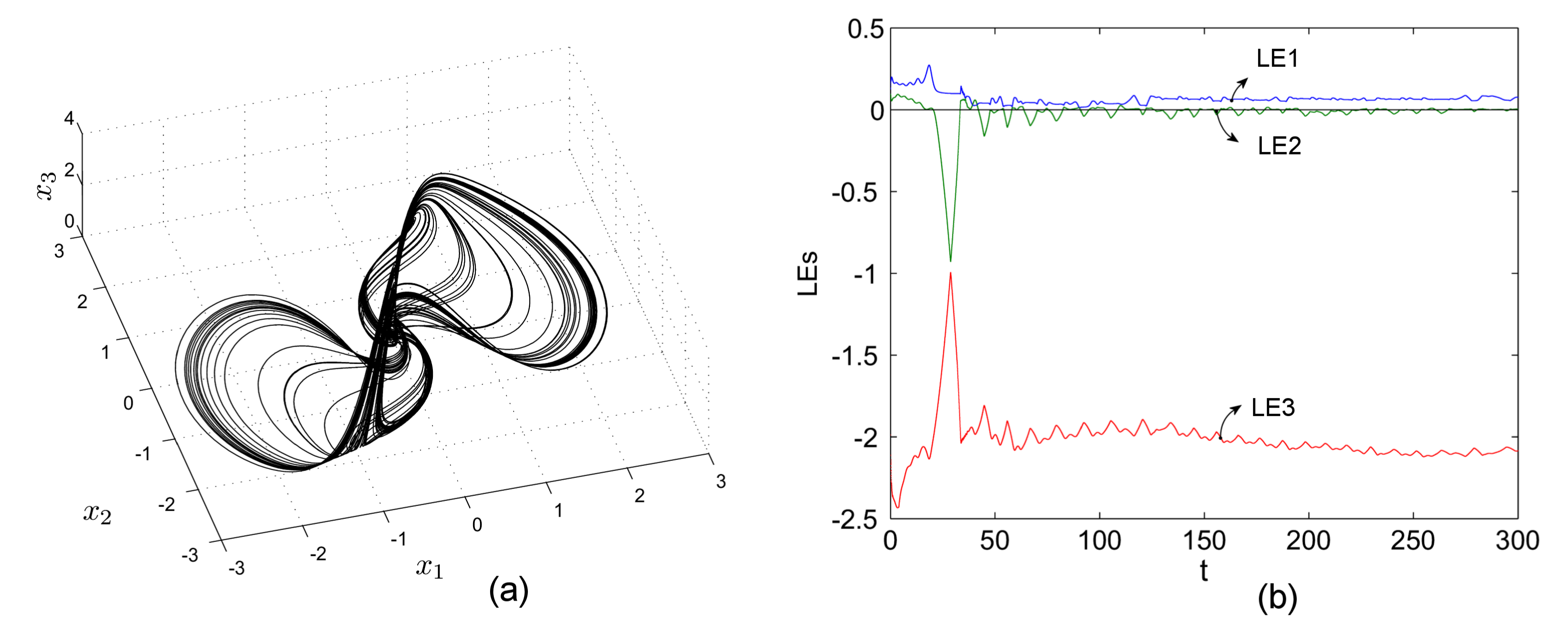
Figure 1: (a) A chaotic attractor of the RF system of FO, for $q=0.999$. (b) Dynamics of the LEs.

With the following parameters, one obtains the chaotic attractor in Fig. 1 (a):

⬇

[t,x]=FDE12(0.999,@RF,0,1500,[0.1;0.1;0.1],...

0.01);

To note that FDE12.m requires the entry, x0, as a column vector [x10,x20,x30]’ or, similarly, [x10;x20;x30]. Also, the returned exit, x, is a column vector.

2.2 Algorithm for LEs of the FO system (1)

Hereafter the finite-time local LEs of FO are called LEs.

The existence of the variational equations necessary to determine LEs is ensured by the following Theorem Li et al. [2010]

Theorem 2.2.

System (1) has the following variational equations which define the LEs

$$\begin{array}[]{l}D_{*}^{q}\Phi(t)=D_{x}f(x)\Phi(t),\\ \Phi(0)=I,\end{array}$$ (2)

where $\Phi$ is the matrix solution of the system (1), $D_{x}$ is the Jacobian of $f$ and $I$ is the identity matrix.

Further we assume that for the matrix $\Phi(t)$ the cocycle property takes place.

Input : 

-$ne$ $\triangleright$ number of equations

-$x\_start$ $\triangleright$ $n_{e}$ initial conditions of (1)

-$t\_start$, $t\_end$ $\triangleright$ time span

-$h\_norm$ $\triangleright$ Normalization step-size

$n\_it\leftarrow$ $(t\_end-t\_start)/h\_norm$ $\triangleright$ iterations number

for $i\leftarrow$ $ne+1$ to $ne(ne+1)$ do

      $x(i)=1.0$ $\triangleright$ initial conditions of (2)

end for

$t\leftarrow t\_start$

for $i\leftarrow$ $1$ to $n\_it$ do

         $x\leftarrow$ integration of FO systems (1)-(2)

      $t\leftarrow t+h\_norm$

      $zn(1),...,zn(ne)\leftarrow$ Gram-Schmidt procedure

      $s(1)\leftarrow 0$

      for $k\leftarrow$ $1$ to $ne$ do

             $s(k)\leftarrow$ $s(k)+log(zn(k))$ $\triangleright$ vector magnitudes

            $LE(k)\leftarrow$ $s(k)/(t-t\_start)$ $\triangleright$ LEs

       end for

      

end for

Output:LE

Algorithm 1 Algorithm for LEs of FO system (1)

Therefore, the algorithm to determine the LEs of the system (1) becomes similar to the case of integer order.

Lyapunov exponents measure the exponential growth, or decay, of infinitesimal phase-space perturbations of a chaotic dynamical system.

The algorithm for numerical evaluation of LEs utilized in this paper, has been proposed in the seminal works of Benettin et al. Benettin et al. [1980] (see also Shimada & Nagashima [1979]), one of the the first work to propose a Gram-Schmidt orthogonalization procedure to compute LEs for continuous systems of integer order, as described in Eckmann & Ruelle [1985]), and by Wolf et al. Wolf et al. [1985b] (see also Eckmann et al. [1986]).

The algorithm to find all LEs, described as a Fortran code by Wolf et al. Wolf et al. [1985b], and also as a Basic code in Baker & Gollub [1990], solves the equations of motion under perturbations and periodic orthonormalization.

To note that the accuracy and reliability of numerically determined LEs depend on initial conditions, on the selection of the perturbations, performances of the utilized integration numerical method and also on orthonormalization step size. A long-time numerical calculation of the leading Lyapunov exponent requires rescaling the distance between nearby trajectories, in order to keep the separation within the linearized flow range. To avoid overflow, one calculates the divergence of nearby trajectories for finite timesteps and renormalizes to unity after a finite number of steps (Gram-Schmidt procedure Eckmann & Ruelle [1985]; Christiansen & Rugh [1997]).

Therefore, the main steps to determine numerically the LEs are: numerical integration of the FO system (1) together with the variational system (2) (i.e. the extended system), Gram-Schmidt procedure and picking up the exponents during the renormalization procedure, the LEs being determined as the average of the logarithm of the stretching factor of each perturbation, steps presented in Algorithm 1.

3 The Matlab code for LEs

Consider the following general assumptions:

• The considered systems, modeled by the IVP (1), are autonomous;

• The system (1) is of commensurate order: $q_{1}=q_{2}=...=q_{ne}=q$;

• In the case of chaotic behavior, the fractional-order has been chosen close to $1$, such that chaos is significant.

• The right hand side of system (1), $f$, is smooth enough.

• Because of the space restrictions, only the main programs code are presented, and indications on how to write the other ones.

A simple way to build in Matlab language the algorithm for FO systems, the program FO_Lyapunov.m (Appendix A), was to modify either some existing program, e.g., the program lyapunov.m Govorukhin [2004], which is a Matlab variant of the original LEs algorithm proposed in Benettin et al. [1980] or Wolf et al. [1985b] or, similarly, to translate in Matlab the BASIC program Baker & Gollub [1990], a close variant of the original algorithm) or, also, the Fortran code proposed by Wolf et all in Wolf et al. [1985b], and modify it for FDEs.

The program, called FO_Lyapunov.m, is launched with the following command line:

⬇

[t,LE]=FO_Lyapunov(ne,@ext_fcn,t_start,h_norm,...

t_end,x_start,h,q,out);

where ne represents the equations (and state variables) number, ext$\_$fcn.m the function containing the extended system (1)-(2), t$\_$start and t$\_$end the time span, h$\_$norm the normalization step, x$\_$start the initial condition (as column vector), h the step size of FDE12.m, and out indicates the steps number when intermediate values of time and LEs are printed (for out=0, no intermediate results will be printed out).

As shown in the algorithm for LEs (Algorithm 1), it is necessary to solve the extended system (1)-(2) of FO (yellow line) which is given in the function ext_fcn.m. In this file, beside the right hand side function f of the system (1), the Jacobi matrix J should be included (see Appendix B where the function for the RF system is presented).

The program plots the time evolutions of the LEs.

4 Numerical tests

Beyond numerical artifacts that might occur when numerically integrating a system of ODEs of integer order, notions such as “shadowing time” and “maximally effective computational time” reveal that it is possible to have reliable numerical simulations only on a relative finite-time interval (see, e.g., Sarra & Meador [2011]; Wang et al. [2012]). The case of FO systems is even more delicate. In this paper we have considered generally $t\in[0,300]$ and, for the Lorenz system, $t\in[0,500]$.

• Let consider the function for the RF system, LE_RF.m, which include the extended system (1)-(2) (Appendix B). Because ne=3, beside the 3 variables x(1),x(2),x(3) required by the numerical solution of the original system (1), the matrix solution of the system (2) requires other more ne$\times$ne=9 variables from the total of ne(ne+1)=12 variables: x(1:12), f=zeros(size(x))=zeros(12), where f loads the first ne=3 righthand side expressions of system (1), and the ne$\times$ne=9 righthand side expressions of the variational system (2).

  For example, for the RF system, with the following command line:

  ⬇

  [t,LE]=FO_Lyapunov(3,@LE_RF,0,0.02,300,...

  [0.1;0.1;0.1],0.005,0.999,1000);

  one obtains the intermediary results printed every out=1000 h$\_$norm steps, presented in Table 1 (see also Fig. 1 (b) where the dynamics of the LEs are drawn).

  ⬇

  10.00 0.1611 0.0660 -2.1614

  20.00 0.1923 0.0069 -2.0503

  30.00 0.0984 -0.7397 -1.1817

  40.00 0.0248 0.0542 -1.9761

  50.00 0.0440 -0.0168 -1.9867

  60.00 0.0697 -0.0006 -2.0701

  70.00 0.0354 -0.0116 -2.0167

  80.00 0.0331 -0.0618 -1.9360

  90.00 0.0201 0.0125 -1.9754

  100.00 0.0429 0.0112 -1.9794

  110.00 0.0337 0.0252 -1.9698

  120.00 0.0262 -0.0213 -1.9038

  130.00 0.0624 -0.0043 -1.9537

  140.00 0.0660 -0.0029 -1.9811

  150.00 0.0645 -0.0010 -2.0008

  160.00 0.0743 0.0018 -2.0304

  170.00 0.0710 -0.0009 -2.0394

  180.00 0.0583 0.0139 -2.0548

  190.00 0.0678 0.0042 -2.0665

  200.00 0.0662 -0.0217 -2.0498

  210.00 0.0628 -0.0155 -2.0622

  220.00 0.0602 -0.0125 -2.0715

  230.00 0.0570 -0.0222 -2.0666

  240.00 0.0643 -0.0222 -2.0813

  250.00 0.0639 -0.0079 -2.1020

  260.00 0.0623 0.0045 -2.1121

  270.00 0.0630 0.0006 -2.0987

  280.00 0.0551 -0.0036 -2.0771

  290.00 0.0761 0.0009 -2.0937

  300.00 0.0749 0.0018 -2.0850

  Listing 1: Caption Text

  Table 1. For $t\in[0,300]$, the RF system has LE = (0.0749, 0.0018, -2.0850) (last line, blue).

• If one considers the Lorenz system

  $$\begin{array}[]{l}D_{*}^{q}x_{1}=\sigma(x(2)-x(1)),\\ D_{*}^{q}x_{2}=-x(1)x(3)+px(1)-x(2)\\ D_{*}^{q}x_{3}=x(1)x(2)-\beta x(3);\end{array}$$ (3)

  with $q=0.985$ and the standard parameters $\sigma=10$, $\beta=8/3$ and the bifurcation parameter $p=200$, after some neglected transients, one obtains an apparently stable cycle (see Fig. 2 (a) and Remark 2.1 (ii)).

  To obtain the LEs one write the following command line:

  ⬇

  [t,LE]=FO_Lyapunov(3,@LE_Lorenz,0,5,500,...

  [0.1;0.1;0.1],0.001,0.985,10);

  Listing 2: Caption Text

  which gives LE=(-0.0026, -0.0870, -1.6225). The function LE$\_$Lorenz.m can be obtained similarly with LE$\_$RF.m. The time evolution of the LEs is presented in Table 2 (see also Fig. 2 (b)).

  ⬇

  50.00 0.1759 -0.1591 -1.5683

  100.00 0.0611 -0.1108 -1.6050

  150.00 0.0346 -0.0927 -1.6300

  200.00 0.0215 -0.0877 -1.6288

  250.00 0.0135 -0.0866 -1.6269

  300.00 0.0082 -0.0865 -1.6255

  350.00 0.0043 -0.0866 -1.6244

  400.00 0.0014 -0.0867 -1.6236

  450.00 -0.0008 -0.0869 -1.6230

  500.00 -0.0026 -0.0870 -1.6225

  Listing 3: Caption Text

  Table 2. Time evolution of the LEs for the Lorenz system. LE=(-0.0026, -0.0870, -1.6225).

• Consider next the non-smooth 4-dimensional system Danca et al. [2018a]

  $$\begin{array}[]{cl}D_{*}^{q}x_{1}=&-x_{1}+x_{2},\\ D_{*}^{q}x_{2}=&-x_{3}\operatorname{sgn}(x_{1})+x_{4},\\ D_{*}^{q}x_{3}=&|x_{1}|-a,\\ D_{*}^{q}x_{4}=&-bx_{2},\end{array}$$ (4)

  with $a=1$, $b=0.5$ and $q=0.98$.

  With the command line:

  ⬇

  [t,LE]=FO_Lyapunov(4,@LE_4d,0,0.02,300,...

  [0.1;0.1;0.1;0.1],0.005,0.98,1000);

  Listing 4: Caption Text

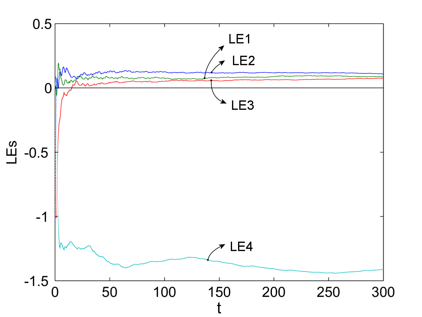
Figure 3: Dynamics of the LEs of the 4-dimensional system of FO (4).

  one obtains LE=(0.1262, 0.0846, 0.0778, -1.5244) (Fig. 3).

  For this example, ne=4, the number of the variables is $20$ and, therefore, compared with systems with ne=3, the function file, LE$\_$4d.m, must be modified accordingly (compare the red line in LE$\_$RF.m). Also, in order to obtain the printed intermediated values of LEs, in the FO$\_$Lyapunov.m, the fprintf command, must be modified by adding one supplementary specifier %10.3f.

  Because from the four LEs, the system admits three positive LEs, it can be considered as hyperchaotic (see Danca et al. [2018b] for a discussion about the number of positive LEs of hyperchaotic systems).

  Remark 4.1.

  Note that because the system is not smooth and also discontinuous, the correct numerical integration required for this system cannot be done without a previous smooth approximation Danca et al. [2018a]. Thus, like all numerical methods for FDEs which are designed for continuous dynamical systems, the integrator FDE12 cannot be utilized in this case without the mentioned approximation. Also, without a smooth approximation, the Jacobian matrix, utilized in the Benettin-Wolf algorithm, cannot be determined.

• LEs can be also plotted as function of the bifurcation parameter $p$ for $p\in[p_{min},p_{max}]$ (program run$\_$Lyapunov$\_$p.m, Appendix C). The program uses a slightly modified variant of FO$\_$Lyapunov.m, which is called FO$\_$Lyapunov$\_$p.m. To obtain FO$\_$Lyapunov$\_$p.m from FO$\_$Lyapunov.m, the following modifications have to be done:

  • The header line of the code FO$\_$Lyapunov.m is replaced with the following line (to note that the output t and the input out are no more necessary)

    ⬇

    function LE=FO_Lyapunov_p(ne,ext_fcn_p,...

    t_start,h_norm,t_end,x_start,h,q,p);

    Listing 5: Caption Text

  • the printing and plotting lines (*) (red color) are deleted;

  • the rest of the lines remain the same;

  The m-file containing the extended system, ext$\_$fcn$\_$p.m, for the RF system, is presented in Appendix D. Passing the parameter $p$ between these codes, can be easily realized due of the facilities of the program FDE12 (see FDE12).

  For example, for the RF system, for $p\in[1.1,1.3]$, for $1000$ values of $p$ ($n=1000$), with the following command

  ⬇

  run_FO_Lyapunov_p(3,@LE_RF_p,0,0.02,200,...

  [0.1;0.1;0.1],0.002,0.998,1.1,1.3,800)

  Listing 6: Caption Text

  one obtains the evolution of the LEs drawn in Fig. 4 (a).

• LEs can be plotted also as function of the fractional order q (program run$\_$Lyapunov$\_$q.m in Appendix E). The used program FO$\_$Lyapunov$\_$q, is obtained from FO$\_$Lyapunov with the following modifications:

  • The header line of the code is replaced with the following line (to note that the input out is no more necessary);

    ⬇

    function [t,LE]=FO_Lyapunov_q(ne,ext_fcn,...t_start,h_norm,t_end,x_start,h,q);

    Listing 7: Caption Text

  • the printing and plotting lines (*) (red color) are deleted;

  • the rest of the lines remain the same;

  The function containing the extended system, ext$\_$fcn.m, does not require any modification.

  For example, for the RF system, with the command

  ⬇

  run_FO_Lypaunov_q(3,@LE_RF,0,0.05,150,...

  [0.1;0.1;0.1],0.002,0.9,1,800)

  Listing 8: Caption Text

  one obtains the LEs plotted in Fig. 4 (b).

  Remark 4.2.

  The presented programs can be optimized especially in the cases of FO$\_$Lyapunov$\_$p.m and FO$\_$Lyapunov$\_$q.m. A simple improvement was to use while loop (instead for) which for these two programs reduce substantially the computational time. However, every parameter $p$ (or order $q$) step, several constant parameters are shared between programs, fact which slows significantly the programs. Therefore, supplementary optimization should be done.

• Another potential application of the proposed LEs algorithm, is to represent the LEs as function of two variables: the order $q$ and the bifurcation parameter $p$.

  Let the Chen system

  $$\begin{array}[]{l}D_{*}^{q}x_{1}=a(x_{2}-x_{1}),\\ D_{*}^{q}x_{2}=(p-a)x_{1}-x_{1}x_{3}+cx_{2},\\ D_{*}^{q}x_{3}=x_{1}x_{2}-bx_{3},\end{array}$$

  with parameters $a=35$, $b=3$ and $q$ and $p$ variables. By considering $S_{i}:=LE(q,c)$, for $i=1,2,3$, for $q\in[0.9,1]$ and $p\in[20,30]$, the obtained surfaces are plotted in Fig. 5 (see Danca et al. [2018b] where the algorithm to obtain LEs as surfaces is described). One can see that there exists a unique positive LE (red surface, $S_{1}$) for all values of the considered parameter $c$ but only for some fractional order values $q$, for which $S_{1}$ is situated over the horizontal plane LE=0, where LEs are zero. Also, one can see that $S_{2}$, which is almost identic to $S_{1}$ when the underlying LE1,2, are negative, becomes zero for a relative large values of $q$ and $p$, when $S_{2}$ separates from $S_{1}$ and identify (with the underlying numerical error) with the plane LE=0.

5 Conclusion and discussion

Starting from an existing variant for integer-order system, in this paper, based on the Benettin-Wolf algorithm, we proposed a Matlab program to determine numerically finite-time local LEs for FO systems.

Due to inherent numerical errors, the algorithm should be utilized with precaution. As known, among the numerical errors, the results depends strongly on the initial conditions, time integration interval and, especially, on the renormalization step size h$\_$norm.

The relative large numerical errors of the Benettin-Wolf algorithm, which for the considered examples was of order of $1.E-2$, can be observed in the cases when one knows that the system presents a numerically periodic cycle (see Remark 2.1 (ii)), when the maximum LE should be zero. For example, the Lorenz system, which for $p=200$ presents such apparently stable cycle (see Fig. 2 (a)), has the maximum LE zero only with two precise decimals. Actually, in general, three precise decimals for zero LEs are extremely rare. Note that this zero value, appears only for h$\_$norm=5 and a smaller integration step size, $h=0.001$ and only for a larger time interval [0,500]. Therefore, if no special improvements of numerical integration are implemented, with Benettin-Wolf algorithm, for integer but also for fractional order systems, two or three decimals are the maximal expected number of decimals.

One of the most important algorithm variable, is h$\_$norm, which determines the normalization moments influences the results. This dependence can be also deduced from the example of the RF system. With h=0.005 and h$\_$norm=0.005 one obtains LEs=(0.0631, 0.0031, -2.0774), while with the same stapsize, h=0.005, but h$\_$norm=0.5, LEs=(0.0643, 0.0026, -1.8254).

Since on our best knowledge, there is not criterion to choose precisely h$\_$norm, the recommended way would be to realize several tests to choose the value for which slightly modifications does not change significantly the results.

In the case of fixed step-size integration numerical methods, like the considered FDE12, h$\_$norm can be chosen as depending on the step size h. Therefore, as Fig. 6 shows, h$\_$norm could be multiple of integration step size h ($\varepsilon$ represents the perturbation between nearly two trajectories $x$ and $\bar{x}$).

Regarding the Gram-Schmidt procedure, in order to speed up the code, one can use the QR decomposition based on the Householder transformation: [Q, R] = qr(A). To have matrix $R$ with positive diagonal elements, one can additionally use Q = Q*diag(sign(diag(R))); R = R*diag(sign(diag(R))). See also Ramasubramanian & Sriram [2000].

The integration step-size of FDE12, $h$, plays an important role. As the documentation of the program specifies, there exists the possibility to increase the performances of the numerical integration, but in time integration detriment.

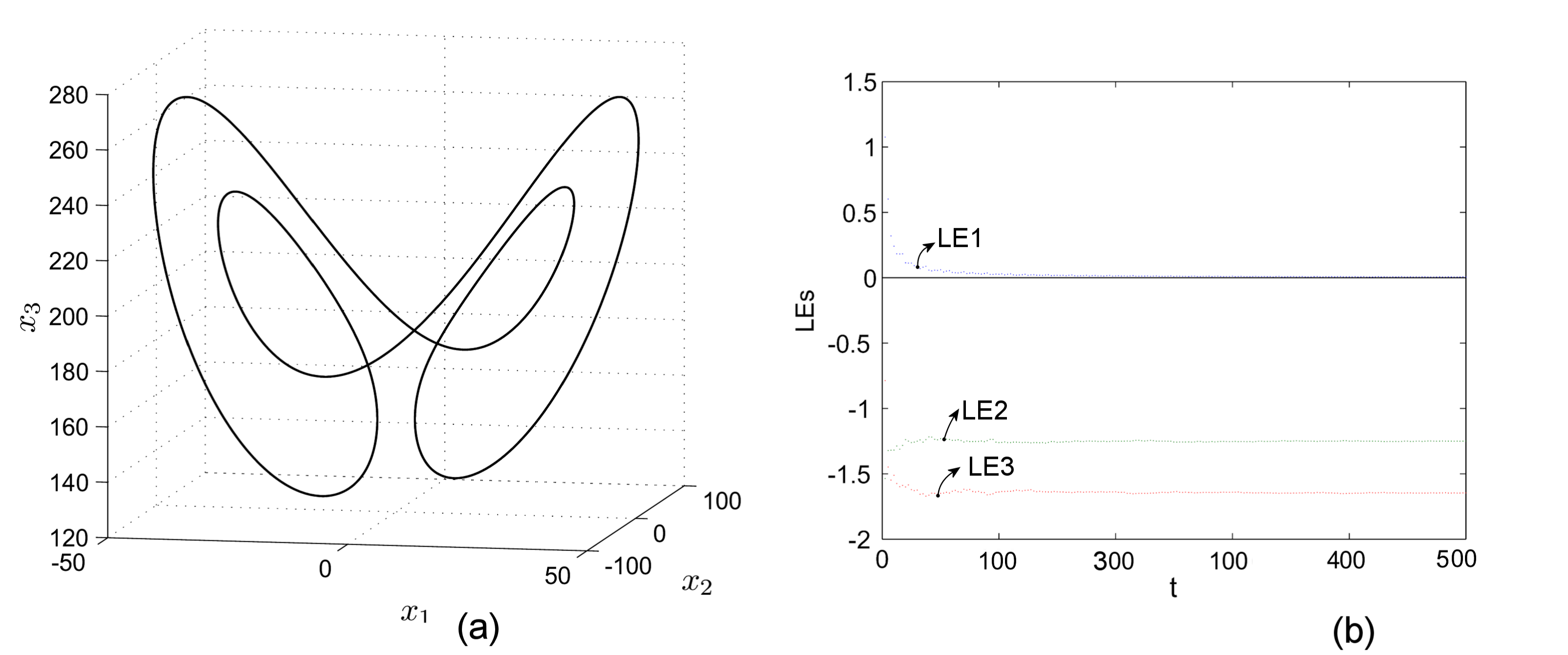
Figure 2: (a) An apparently stable cycle of the generalized Lorenz system of FO, for $q=0.985$. (b) Dynamics of the LEs.

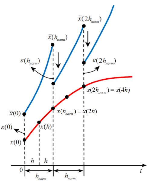
Figure 4: Perturbation and rescaling of a nearby trajectory, after every $h_{norm}$ steps, considered as multiple of $h$ (here $h_{norm}=2h$, sketch).

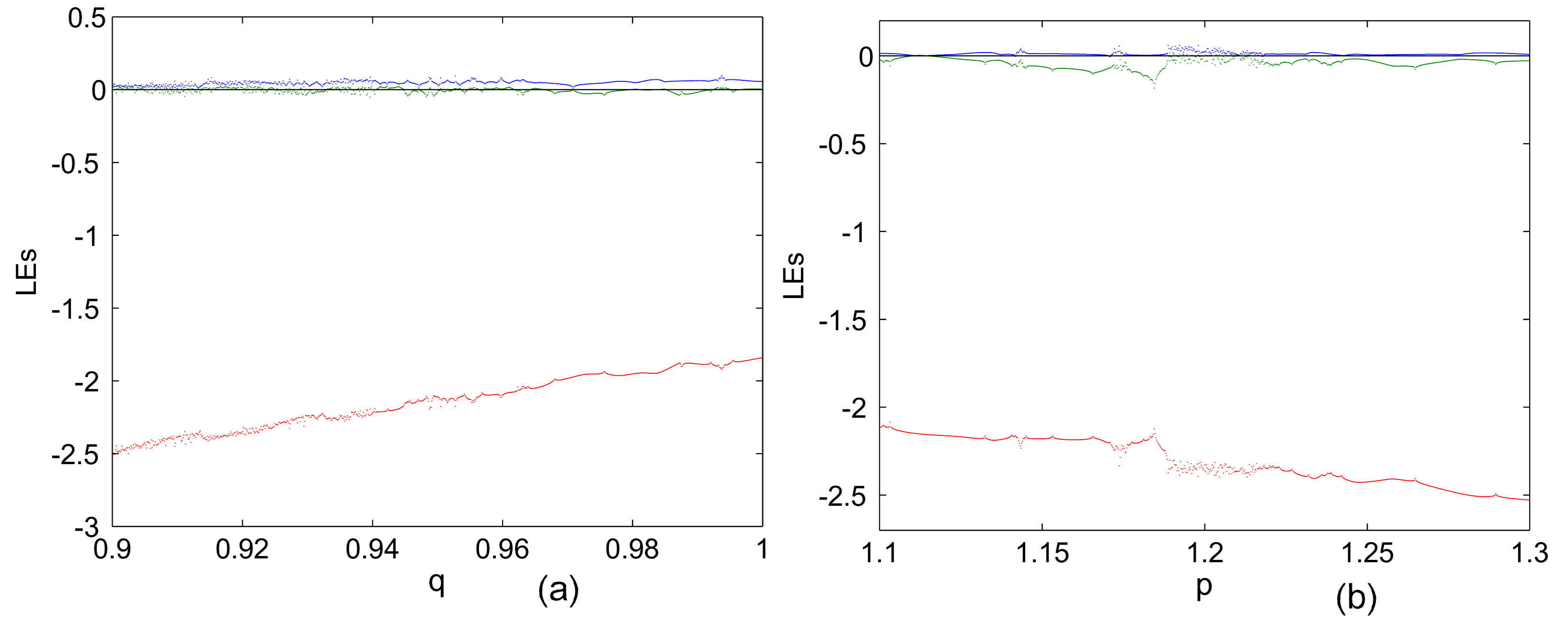
Figure 5: LEs of RF system. (a) LEs as function of $q$ for $q\in[0.9,1]$. (b) LEs as function of $p$ for $p\in[1.1,1.3]$.

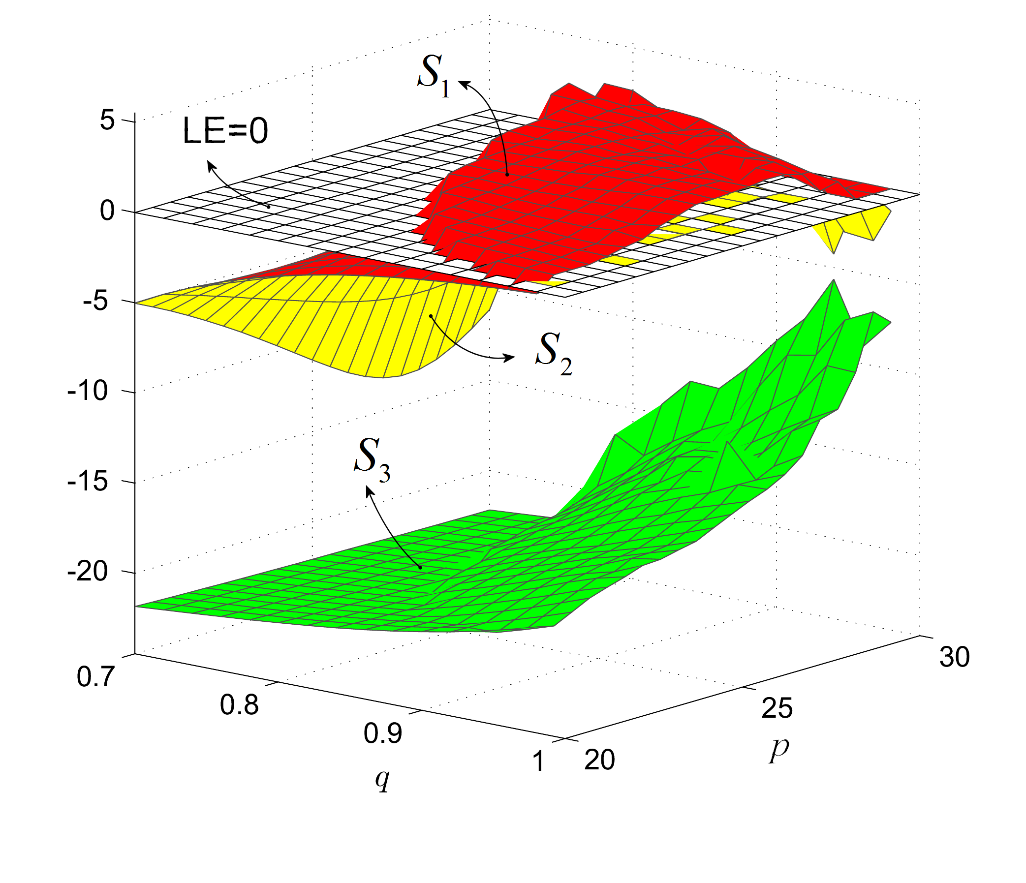
Figure 6: LEs of Chen’s system of FO represented by function of two variables: $q$ and parameter $p$. Surfaces $S_{i}$, for $i=1,2,3$, represents $LE(q,p)$.

Appendices

A Program for LEs of FO

⬇

function [t,LE]=FO_Lyapunov(ne,ext_fcn,t_start,h_norm,t_end,x_start,h,q,out);

%

% Program to compute LEs of systems of FO.

%

% The program uses a fast variant of the

% predictor-corrector Adams-Bashforth-Moulton,

% "FDE12.m" for FDEs, by Roberto Garrappa:

%

% https://goo.gl/XScYmi

%

% m-file required: FDE12 and

% the function containing the extended system

% (see e.g. LE_RF.m).

%

% FO_Lyapunov.m was developed, by

% modifying the program Lyapunov.m,

% by V.N. Govorukhin:

%

% https://goo.gl/wZVCtg

%

% FO_Lyapunov.m, FDE12.m and LE_RF.m

% must be in the same folder.

%

% How to use it:

% [t,LE]=FO_Lyapunov(ne,ext_fcn,t_start,...

% h_norm,t_end,x_start,h,q,out);

%

% Input:

% ne - system dimension;

% ext_fcn - function containing the extended

% system;

% t_start, t_end - time span;

% h_norm - step for Gram-Schmidt

% renormalization;

% x_start - initial condition;

% outp - priniting step of LEs;

% ioutp==0 - no print.

%

% Output:

% t - time values;

% LE Lyapunov exponents to each time value.

%

% Example of use for the RF system:

% [t,LE]=FO_Lyapunov(3,@LE_RF,0,0.02,300,...

% [0.1;0;1;0.1],0.005,0.999,1000);

%

% The program is presented in:

%

% Marius-F. Danca and N. Kuznetsov,

% Matlab code for Lyapunov exponents of

% fractional order systems

%

%

hold on;

% Memory allocation

x=zeros(ne*(ne+1),1);

x0=x;

c=zeros(ne,1);

gsc=c; zn=c;

n_it = round((t_end-t_start)/h_norm);

% Initial values

x(1:ne)=x_start;

i=1;

while i<=ne

x((ne+1)*i)=1.0;

i=i+1;

end

t=t_start;

% Main loop

it=1;

while it<=n_it

% Solution of extended ODE system

[T,Y] = FDE12(q,ext_fcn,t,t+h_norm,x,h);

t=t+h_norm;

Y=transpose(Y);

x=Y(size(Y,1),:); %solution at t+h_norm

i=1;

while i<=ne

j=1;

while j<=ne;

x0(ne*i+j)=x(ne*j+i);

j=j+1;

end;

i=i+1;

end;

% orthonormal Gram-Schmidt basis

zn(1)=0.0;

j=1;

while j<=ne

zn(1)=zn(1)+x0(ne*j+1)*x0(ne*j+1);

j=j+1;

end;

zn(1)=sqrt(zn(1));

j=1;

while j<=ne

x0(ne*j+1)=x0(ne*j+1)/zn(1);

j=j+1;

end

j=2;

while j<=ne

k=1;

while k<=j-1

gsc(k)=0.0;

l=1;

while l<=ne;

gsc(k)=gsc(k)+x0(ne*l+j)*x0(ne*l+k);

l=l+1;

end

k=k+1;

end

k=1;

while k<=ne

l=1;

while l<=j-1

x0(ne*k+j)=x0(ne*k+j)-gsc(l)*x0(ne*k+l);

l=l+1;

end

k=k+1;

end;

zn(j)=0.0;

k=1;

while k<=ne

zn(j)=zn(j)+x0(ne*k+j)*x0(ne*k+j);

k=k+1;

end

zn(j)=sqrt(zn(j));

k=1;

while k<=ne

x0(ne*k+j)=x0(ne*k+j)/zn(j);

k=k+1;

end

j=j+1;

end

% update running vector magnitudes

k=1;

while k<=ne;

c(k)=c(k)+log(zn(k));

k=k+1;

end;

% normalize exponent

k=1;

while k<=ne

LE(k)=c(k)/(t-t_start);

k=k+1;

end

i=1;

while i<=ne

j=1;

while j<=ne;

x(ne*j+i)=x0(ne*i+j);

j=j+1;

end

i=i+1;

end;

x=transpose(x);

it=it+1;

% print and plot the results

if (mod(it,out)==0) % (*)

fprintf(’%10.2f %10.4f %10.4f...

%10.4f\n’,[t,LE]); % (*)

end; % (*)

plot(t,LE) % (*)

end

% displays the box outline around axes

xlabel(’t’,’fontsize’,16) % (*)

ylabel(’LEs’,’fontsize’,14) % (*)

set(gca,’fontsize’,14)% (*)

box on;% (*)

line([0,t],[0,0],’color’,’k’)% (*)

B Function LE_RF.m

⬇

function f=LE_RF(t,x)

%Output data must be a column vector

f=zeros(size(x));

%variables allocated to the variational equations

X= [x(4), x(7), x(10);

x(5), x(8), x(11);

x(6), x(9), x(12)];

%RF equations

f(1)=x(2)*(x(3)-1+x(1)*x(1))+0.1*x(1);

f(2)=x(1)*(3*x(3)+1-x(1)*x(1))+0.1*x(2);

f(3)=-2*x(3)*(0.98+x(1)*x(2));

%Jacobian matrix

J=[2*x(1)*x(2)+0.1, x(1)*x(1)+x(3)-1, x(2);

-3*x(1)*x(1)+3*x(3)+1,0.1,3*x(1);

-2*x(2)*x(3),-2*x(1)*x(3),-2*(x(1)*x(2)+0.98)];

%Righthand side of variational equations

f(4:12)=J*X; % To be modified if ne>3

C Program for LEs as function on $p$

⬇

function run_Lyapunov_p(ne,ext_fcn,t_start,h_norm,t_end,x_start,h,q,p_min,p_max,n);

hold on;

p_step=(p_max-p_min)/n

p=p_min;

while p<=p_max

LE=FO_Lyapunov_p(ne,ext_fcn,t_start,h_norm,t_end,x_start,h,q,p);

p=p+p_step

plot(p,LE);

end

D Function LE_RF_p.m

⬇

function f=LE_RF_p(t,x,p)

%p is the parameter

f=zeros(size(x));

X= [x(4), x(7), x(10);

x(5), x(8), x(11);

x(6), x(9), x(12)];

%RF equations

f(1)=x(2)*(x(3)-1+x(1)*x(1))+0.1*x(1);

f(2)=x(1)*(3*x(3)+1-x(1)*x(1))+0.1*x(2);

f(3)=-2*x(3)*(p+x(1)*x(2));

%Jacobian matrix

J=[2*x(1)*x(2)+0.1, x(1)*x(1)+x(3)-1, x(2);

-3*x(1)*x(1)+3*x(3)+1,0.1,3*x(1);

-2*x(2)*x(3),-2*x(1)*x(3),-2*(x(1)*x(2)+p)];

f(4:12)=J*X; % To be modified if ne>3

E Program for LEs as function of $q$

⬇

function run_FO_Lyapunov_q(ne,ext_fcn,t_start,h_norm,t_end,x_start,h,q_min,q_max,n);

hold on;

q_step=(q_max-q_min)/n;

q=q_min;

while q<q_max

[t,LE]=FO_Lyapunov_q(ne,ext_fcn,t_start,h_norm,t_end,x_start,h,q);

q=q+q_step;

fprintf(’q=%10.4f\n %10.4f’, q);

plot(q,LE);

end

References

- Abarbanel et al. [1993] Abarbanel, H., Brown, R., Sidorowich, J. & Tsimring, L. [1993] “The analysis of observed chaotic data in physical systems,” Reviews of Modern Physics 65, 1331–1392.
- Baker & Gollub [1990] Baker, G. & Gollub, P. [1990] Chaotic Dynamics: An Introduction (Cambridge University Press, Cambridge).
- Barreira & Pesin [2001] Barreira, L. & Pesin, Y. [2001] “Lectures on Lyapunov exponents and smooth ergodic theory,” Proc. of. Symposia in Pure Math. (AMS), pp. 3–89.
- Benettin et al. [1980] Benettin, G., Galgani, L., Giorgilli, A. & Strelcyn, J.-M. [1980] “Lyapunov characteristic exponents for smooth dynamical systems and for hamiltonian systems. A method for computing all of them. Part II: Numerical application,” Meccanica 15, 21–30.
- Bylov et al. [1966] Bylov, B. E., Vinograd, R. E., Grobman, D. M. & Nemytskii, V. V. [1966] Theory of characteristic exponents and its applications to problems of stability (in Russian) (Nauka, Moscow).
- Caputo [1967] Caputo, M. [1967] “Linear models of dissipation whose Q is almost frequency independent-II,” Geophysical Journal of the Royal Astronomical Society 13, 529–539.
- Christiansen & Rugh [1997] Christiansen, F. & Rugh, H. [1997] “Computing Lyapunov spectra with continuous gram-schmidt orthonormalization,” Nonlinearity 10, 1063–1072.
- Cvitanović et al. [2016] Cvitanović, P., Artuso, R., Mainieri, R., Tanner, G. & Vattay, G. [2016] Chaos: Classical and Quantum (Niels Bohr Institute, Copenhagen), http://ChaosBook.org.
- Czornik et al. [2013] Czornik, A., Nawrat, A. & Niezabitowski, M. [2013] “Lyapunov exponents for discrete time-varying systems,” Studies in Computational Intelligence 440, 29–44.
- Danca [2016] Danca, M.-F. [2016] “Hidden transient chaotic attractors of Rabinovich–Fabrikant system,” Nonlinear Dynamics 86, 1263–1270.
- Danca et al. [2018a] Danca, M.-F., Fečkan, M., Kuznetsov, N. & Chen, G. [2018a] “Complex dynamics, hidden attractors and continuous approximation of a fractional-order hyperchaotic PWC system,” Nonlinear Dynamics 91, 2523–2540.
- Danca et al. [2018b] Danca, M.-F., Fečkan, M., Kuznetsov, N. V. & Chen, G. [2018b] “Fractional-order PWC systems without zero Lyapunov exponents,” Nonlinear Dynamics Doi:10.1007/s11071-018-4108-2.
- Diethelm [2014] Diethelm, K. [2014] “An extension of the well-posedness concept for fractional differential equations of caputo s type,” Applicable Analysis 93, 2126–2135.
- Diethelm & Ford [2002] Diethelm, K. & Ford, N. [2002] “Analysis of fractional differential equations,” Journal of Mathematical Analysis and Applications 265, 229–248.
- Diethelm et al. [2002] Diethelm, K., Ford, N. & Freed, A. [2002] “A predictor-corrector approach for the numerical solution of fractional differential equations,” Nonlinear Dynamics 29, 3–22.
- Eckmann et al. [1986] Eckmann, J. P., Kamphorst, S. O., Ruelle, D. & Ciliberto, S. [1986] “Liapunov exponents from time series,” Phys. Rev. A 34, 4971–4979.
- Eckmann & Ruelle [1985] Eckmann, J.-P. & Ruelle, D. [1985] “Ergodic theory of chaos and strange attractors,” Reviews of Modern Physics 57, 617–656.
- Frederickson et al. [1983] Frederickson, P., Kaplan, J., Yorke, E. & Yorke, J. [1983] “The Liapunov dimension of strange attractors,” Journal of Differential Equations 49, 185–207.
- Garrappa [2012] Garrappa, R. [2012] “Predictor-corrector PECE method for fractional differential equations,” https://www.mathworks.com/matlabcentral/fileexchange/32918-predictor-corrector-pece-method-for-fractional-differential-equations?focused=5235405&tab=function.
- Gorenflo & Mainardi [1997] Gorenflo, R. & Mainardi, F. [1997] “Fractional Calculus,” Fractals and Fractional Calculus in Continuum Mechanics. International Centre for Mechanical Sciences (Courses and Lectures), Vol. 8 (Springer, Vienna).
- Govorukhin [2004] Govorukhin, V. [2004] “Calculation Lyapunov exponents for ODE,” http://www.math.rsu.ru/mexmat/kvm/matds/.
- Hartley et al. [2013] Hartley, T., Lorenzo, C., Trigeassou, J. & Maamri, N. [2013] “Equivalence of history-function based and infinite-dimensional-state initializations for fractional-order operators,” ASME. J. Comput. Nonlinear Dynam. 8, art. num. 041014.
- Hegger et al. [1999] Hegger, R., Kantz, H. & Schreiber, T. [1999] “Practical implementation of nonlinear time series methods: The TISEAN package,” Chaos 9, 413–435.
- Hilbert [1901-1902] Hilbert, D. [1901-1902] “Mathematical problems,” Bull. Amer. Math. Soc. , 437–479.
- Kilbas & Trujillo [2001] Kilbas, A. & Trujillo, J. [2001] “Differential equations of fractional order:methods results and problem i,” Applicable Analysis 78, 153–192.
- Kuznetsov et al. [2016] Kuznetsov, N., Alexeeva, T. & Leonov, G. [2016] “Invariance of Lyapunov exponents and Lyapunov dimension for regular and irregular linearizations,” Nonlinear Dynamics 85, 195–201, 10.1007/s11071-016-2678-4.
- Kuznetsov et al. [2018a] Kuznetsov, N., Leonov, G., Mokaev, T., Prasad, A. & Shrimali, M. [2018a] “Finite-time Lyapunov dimension and hidden attractor of the Rabinovich system,” Nonlinear dynamics https://doi.org/10.1007/s11071-018-4054-z.
- Kuznetsov et al. [2018b] Kuznetsov, N., Leonov, G., Mokaev, T., Prasad, A. & Shrimali, M. [2018b] “Finite-time Lyapunov dimension and hidden attractor of the Rabinovich system,” Nonlinear dynamics https://doi.org/10.1007/s11071-018-4054-z.
- Leonov & Kuznetsov [2007] Leonov, G. & Kuznetsov, N. [2007] “Time-varying linearization and the Perron effects,” International Journal of Bifurcation and Chaos 17, 1079–1107, 10.1142/S0218127407017732.
- Leonov & Kuznetsov [2015] Leonov, G. & Kuznetsov, N. [2015] “On differences and similarities in the analysis of Lorenz, Chen, and Lu systems,” Applied Mathematics and Computation 256, 334–343, 10.1016/j.amc.2014.12.132.
- Leonov et al. [2016] Leonov, G., Kuznetsov, N., Korzhemanova, N. & Kusakin, D. [2016] “Lyapunov dimension formula for the global attractor of the Lorenz system,” Communications in Nonlinear Science and Numerical Simulation 41, 84–103, 10.1016/j.cnsns.2016.04.032.
- Li et al. [2010] Li, C., Gong, Z., Qian, D. & Chen, Y. [2010] “On the bound of the Lyapunov exponents for the fractional differential systems,” Chaos 20, art. num. 016001CHA.
- Lyapunov [1892] Lyapunov, A. [1892] The General Problem of the Stability of Motion (in Russian) (Kharkov), [English transl.: Academic Press, NY, 1966].
- Oldham & Spanier [1974] Oldham, K. & Spanier, J. [1974] The Fractional Calculus: Theory and Applications of Differentiation and Integration to Arbitrary Order (Academic Press, New York).
- Oseledets [1968] Oseledets, V. [1968] “A multiplicative ergodic theorem. Characteristic Ljapunov, exponents of dynamical systems,” Trudy Moskovskogo Matematicheskogo Obshchestva (in Russian) 19, 179–210.
- Pikovsky & Politi [2016] Pikovsky, A. & Politi, A. [2016] Lyapunov Exponents: A Tool to Explore Complex Dynamics (Cambridge University Press).
- Podlubny [1999] Podlubny, I. [1999] Fractional Differential Equations: An Introduction to Fractional Derivatives, Fractional Differential Equations, to Methods of their Solution and some of their Applications, Lecture Notes in Applied and Computational Mechanics (Academic Press, San Diego).
- Podlubny [2002] Podlubny, I. [2002] “Geometric and physical interpretation of fractional integration and fractional differentiation,” Fractional Calculus and Applied Analysis 5, 367–386.
- Ramasubramanian & Sriram [2000] Ramasubramanian, K. & Sriram, M. [2000] “A comparative study of computation of Lyapunov spectra with different algorithms,” Physica D: Nonlinear Phenomena 139, 72–86.
- Sarra & Meador [2011] Sarra, S. & Meador, C. [2011] “On the numerical solution of chaotic dynamical systems using extend precision floating point arithmetic and very high order numerical methods,” Nonlinear Analysis 16, 340 352.
- Shimada & Nagashima [1979] Shimada, I. & Nagashima, T. [1979] “A numerical approach to ergodic problem of dissipative dynamical systems,” Progress of Theoretical Physics 61, 1605–1616.
- Skokos [2010] Skokos, C. [2010] “The Lyapunov characteristic exponents and their computation,” Lecture Notes in Physics 790, 63–135.
- Stuart & Humphries [1998] Stuart, A. & Humphries, A. [1998] Dynamical Systems and Numerical Analysis (Cambridge University Press).
- Tavazoei & Haeri [2009] Tavazoei, M. & Haeri, M. [2009] “A proof for non existence of periodic solutions in time invariant fractional order systems,” Automatica 45, 1886 – 1890.
- Vallejo & Sanjuan [2017] Vallejo, J. & Sanjuan, M. [2017] Predictability of Chaotic Dynamics: A Finite-time Lyapunov Exponents Approach (Springer, Cham, Switzerland).
- Wang et al. [2012] Wang, P., Li, J. & Li, Q. [2012] “Computational uncertainty and the application of a high-performance multiple precision scheme to obtaining the correct reference solution of lorenz equations,” Numerical Algorithms 59, 147–159.
- Wolf et al. [1985a] Wolf, A., Swift, J. B., Swinney, H. L. & Vastano, J. A. [1985a] “Determining Lyapunov exponents from a time series,” Physica D: Nonlinear Phenomena 16, 285–317.
- Wolf et al. [1985b] Wolf, A., Swift, J. B., Swinney, H. L. & Vastano, J. A. [1985b] “Determining Lyapunov exponents from a time series,” Physica D: Nonlinear Phenomena 16, 285–317.
- Zhou [2016] Zhou, Y. [2016] Fractional Evolution Equations and Inclusions: Analysis and Control (Academic Press).