Renewal Monte Carlo:
Renewal theory based reinforcement learning

Jayakumar Subramanian and Aditya Mahajan This work was supported by the Natural Sciences and Engineering Research Council of Canada through NSERC Discovery Accelerator RGPAS 493011-16.The authors are with the Electrical and Computer Engineering Department, McGill University, Montreal, QC H3A 0E9, Canada. (e-mails: jayakumar.subramanian@mail.mcgill.ca, aditya.mahajan@mcgill.ca)
Abstract

In this paper, we present an online reinforcement learning algorithm, called Renewal Monte Carlo (RMC), for infinite horizon Markov decision processes with a designated start state. RMC is a Monte Carlo algorithm and retains the advantages of Monte Carlo methods including low bias, simplicity, and ease of implementation while, at the same time, circumvents their key drawbacks of high variance and delayed (end of episode) updates. The key ideas behind RMC are as follows. First, under any reasonable policy, the reward process is ergodic. So, by renewal theory, the performance of a policy is equal to the ratio of expected discounted reward to the expected discounted time over a regenerative cycle. Second, by carefully examining the expression for performance gradient, we propose a stochastic approximation algorithm that only requires estimates of the expected discounted reward and discounted time over a regenerative cycle and their gradients. We propose two unbiased estimators for evaluating performance gradients—a likelihood ratio based estimator and a simultaneous perturbation based estimator—and show that for both estimators, RMC converges to a locally optimal policy. We generalize the RMC algorithm to post-decision state models and also present a variant that converges faster to an approximately optimal policy. We conclude by presenting numerical experiments on a randomly generated MDP, event-triggered communication, and inventory management.

Index Terms:
Reinforcement learning, Markov decision processes, renewal theory, Monte Carlo methods, policy gradient, stochastic approximation

I Introduction

In recent years, reinforcement learning [1, 2, 3, 4] has emerged as a leading framework to learn how to act optimally in unknown environments. Policy gradient methods [5, 6, 7, 8, 9, 10] have played a prominent role in the success of reinforcement learning. Such methods have two critical components: policy evaluation and policy improvement. In policy evaluation step, the performance of a parameterized policy is evaluated while in the policy improvement step, the policy parameters are updated using stochastic gradient ascent.

Policy gradient methods may be broadly classified as Monte Carlo methods and temporal difference methods. In Monte Carlo methods, performance of a policy is estimated using the discounted return of a single sample path; in temporal difference methods, the value(-action) function is guessed and this guess is iteratively improved using temporal differences. Monte Carlo methods are attractive because they have zero bias, are simple and easy to implement, and work for both discounted and average reward setups as well as for models with continuous state and action spaces. However, they suffer from various drawbacks. First, they have a high variance because a single sample path is used to estimate performance. Second, they are not asymptotically optimal for infinite horizon models because it is effectively assumed that the model is episodic; in infinite horizon models, the trajectory is arbitrarily truncated to treat the model as an episodic model. Third, the policy improvement step cannot be carried out in tandem with policy evaluation. One must wait until the end of the episode to estimate the performance and only then can the policy parameters be updated. It is for these reasons that Monte Carlo methods are largely ignored in the literature on policy gradient methods, which almost exclusively focuses on temporal difference methods such as actor-critic with eligibility traces [3].

In this paper, we propose a Monte Carlo method—which we call Renewal Monte Carlo (RMC)—for infinite horizon Markov decision processes with designated start state. Like Monte Carlo, RMC has low bias, is simple and easy to implement, and works for models with continuous state and action spaces. At the same time, it does not suffer from the drawbacks of typical Monte Carlo methods. RMC is a low-variance online algorithm that works for infinite horizon discounted and average reward setups. One doesn’t have to wait until the end of the episode to carry out the policy improvement step; it can be carried out whenever the system visits the start state (or a neighborhood of it).

Although renewal theory is commonly used to estimate performance of stochastic systems in the simulation optimization community [11, 12], those methods assume that the probability law of the primitive random variables and its weak derivate are known, which is not the case in reinforcement learning. Renewal theory is also commonly used in the engineering literature on queuing theory and systems and control for Markov decision processes (MDPs) with average reward criteria and a known system model. There is some prior work on using renewal theory for reinforcement learning [13, 14], where renewal theory based estimators for the average return and differential value function for average reward MDPs is developed. In RMC, renewal theory is used in a different manner for discounted reward MDPs (and the results generalize to average cost MDPs).

II RMC Algorithm

Consider a Markov decision process (MDP) with state St𝒮subscript𝑆𝑡𝒮S_{t}\in\mathcal{S} and action At𝒜subscript𝐴𝑡𝒜A_{t}\in\mathcal{A}. The system starts in an initial state s0𝒮subscript𝑠0𝒮s_{0}\in\mathcal{S} and at time t𝑡t:

  1. 1.

    there is a controlled transition from Stsubscript𝑆𝑡S_{t} to St+1subscript𝑆𝑡1S_{t+1} according to a transition kernel P(At)𝑃subscript𝐴𝑡P(A_{t});

  2. 2.

    a per-step reward Rt=r(St,At,St+1)subscript𝑅𝑡𝑟subscript𝑆𝑡subscript𝐴𝑡subscript𝑆𝑡1R_{t}=r(S_{t},A_{t},S_{t+1}) is received.

Future is discounted at a rate γ(0,1)𝛾01\gamma\in(0,1).

A (time-homogeneous and Markov) policy π𝜋\pi maps the current state to a distribution on actions, i.e., Atπ(St)similar-tosubscript𝐴𝑡𝜋subscript𝑆𝑡A_{t}\sim\pi(S_{t}). We use π(a|s)𝜋conditional𝑎𝑠\pi(a|s) to denote (At=a|St=s)subscript𝐴𝑡conditional𝑎subscript𝑆𝑡𝑠\mathbb{P}(A_{t}=a|S_{t}=s). The performance of a policy π𝜋\pi is given by

Jπ=𝔼Atπ(St)[t=0γtRt|S0=s0].J_{\pi}=\mathbb{E}_{A_{t}\sim\pi(S_{t})}\biggl{[}\sum_{t=0}^{\infty}\gamma^{t}R_{t}\biggm{|}S_{0}=s_{0}\biggr{]}. (1)

We are interested in identifying an optimal policy, i.e., a policy that maximizes the performance. When 𝒮𝒮\mathcal{S} and 𝒜𝒜\mathcal{A} are Borel spaces, we assume that the model satisfies the standard conditions under which time-homogeneous Markov policies are optimal [15]. In the sequel, we present a sample path based online learning algorithm, which we call Renewal Monte Carlo (RMC), which identifies a locally optimal policy within the class of parameterized policies.

Suppose policies are parameterized by a closed and convex subset ΘΘ\Theta of the Euclidean space. For example, ΘΘ\Theta could be the weight vector in a Gibbs soft-max policy, or the weights of a deep neural network, or the thresholds in a control limit policy, and so on. Given θΘ𝜃Θ\theta\in\Theta, we use πθsubscript𝜋𝜃\pi_{\theta} to denote the policy parameterized by θ𝜃\theta and Jθsubscript𝐽𝜃J_{\theta} to denote Jπθsubscript𝐽subscript𝜋𝜃J_{\pi_{\theta}}. We assume that for all policies πθsubscript𝜋𝜃\pi_{\theta}, θΘ𝜃Θ\theta\in\Theta, the designated start state s0subscript𝑠0s_{0} is positive recurrent.

The typical approach for policy gradient based reinforcement learning is to start with an initial guess θ0Θsubscript𝜃0Θ\theta_{0}\in\Theta and iteratively update it using stochastic gradient ascent. In particular, let ^Jθm^subscript𝐽subscript𝜃𝑚\widehat{\nabla}J_{\theta_{m}} be an unbiased estimator of θJθ|θ=θmevaluated-atsubscript𝜃subscript𝐽𝜃𝜃subscript𝜃𝑚\nabla_{\theta}J_{\theta}\big{|}_{\theta=\theta_{m}}, then update

θm+1=[θm+αm^Jθm]Θsubscript𝜃𝑚1subscriptdelimited-[]subscript𝜃𝑚subscript𝛼𝑚^subscript𝐽subscript𝜃𝑚Θ\theta_{m+1}=\big{[}\theta_{m}+\alpha_{m}\widehat{\nabla}J_{\theta_{m}}\big{]}_{\Theta} (2)

where [θ]Θsubscriptdelimited-[]𝜃Θ[\theta]_{\Theta} denotes the projection of θ𝜃\theta onto ΘΘ\Theta and {αm}m1subscriptsubscript𝛼𝑚𝑚1\{\alpha_{m}\}_{m\geq 1} is the sequence of learning rates that satisfies the standard assumptions of

m=1αm=andm=1αm2<.formulae-sequencesuperscriptsubscript𝑚1subscript𝛼𝑚andsuperscriptsubscript𝑚1superscriptsubscript𝛼𝑚2\sum_{m=1}^{\infty}\alpha_{m}=\infty\quad\text{and}\quad\sum_{m=1}^{\infty}\alpha_{m}^{2}<\infty. (3)

Under mild technical conditions [16], the above iteration converges to a θsuperscript𝜃\theta^{*} that is locally optimal, i.e., θJθ|θ=θ=0evaluated-atsubscript𝜃subscript𝐽𝜃𝜃superscript𝜃0\nabla_{\theta}J_{\theta}\big{|}_{\theta=\theta^{*}}=0. In RMC, we approximate θJθsubscript𝜃subscript𝐽𝜃\nabla_{\theta}J_{\theta} by a Renewal theory based estimator as explained below.

Let τ(n)superscript𝜏𝑛\tau^{(n)} denote the stopping time when the system returns to the start state s0subscript𝑠0s_{0} for the n𝑛n-th time. In particular, let τ(0)=0superscript𝜏00\tau^{(0)}=0 and for n1𝑛1n\geq 1 define

τ(n)=inf{t>τ(n1):st=s0}.superscript𝜏𝑛infimumconditional-set𝑡superscript𝜏𝑛1subscript𝑠𝑡subscript𝑠0\tau^{(n)}=\inf\{t>\tau^{(n-1)}:s_{t}=s_{0}\}.

We call the sequence of (St,At,Rt)subscript𝑆𝑡subscript𝐴𝑡subscript𝑅𝑡(S_{t},A_{t},R_{t}) from τ(n1)superscript𝜏𝑛1\tau^{(n-1)} to τ(n)1superscript𝜏𝑛1{\tau^{(n)}-1} as the n𝑛n-th regenerative cycle. Let 𝖱(n)superscript𝖱𝑛\mathsf{R}^{(n)} and 𝖳(n)superscript𝖳𝑛\mathsf{T}^{(n)} denote the total discounted reward and total discounted time of the n𝑛n-th regenerative cycle, i.e.,

𝖱(n)=Γ(n)t=τ(n1)τ(n)1γtRtand𝖳(n)=Γ(n)t=τ(n1)τ(n)1γt,formulae-sequencesuperscript𝖱𝑛superscriptΓ𝑛subscriptsuperscriptsuperscript𝜏𝑛1𝑡superscript𝜏𝑛1superscript𝛾𝑡subscript𝑅𝑡andsuperscript𝖳𝑛superscriptΓ𝑛subscriptsuperscriptsuperscript𝜏𝑛1𝑡superscript𝜏𝑛1superscript𝛾𝑡\displaystyle\mathsf{R}^{(n)}=\Gamma^{(n)}\smashoperator[r]{\sum_{t=\tau^{(n-1)}}^{\tau^{(n)}-1}}\gamma^{t}R_{t}\quad\text{and}\quad\mathsf{T}^{(n)}=\Gamma^{(n)}\smashoperator[r]{\sum_{t=\tau^{(n-1)}}^{\tau^{(n)}-1}}\gamma^{t}, (4)

where Γ(n)=γτ(n1)superscriptΓ𝑛superscript𝛾superscript𝜏𝑛1\Gamma^{(n)}=\gamma^{-\tau^{(n-1)}}. By the strong Markov property, {𝖱(n)}n1subscriptsuperscript𝖱𝑛𝑛1\{\mathsf{R}^{(n)}\}_{n\geq 1} and {𝖳(n)}n1subscriptsuperscript𝖳𝑛𝑛1\{\mathsf{T}^{(n)}\}_{n\geq 1} are i.i.d. sequences. Let 𝖱θsubscript𝖱𝜃\mathsf{R}_{\theta} and 𝖳θsubscript𝖳𝜃\mathsf{T}_{\theta} denote 𝔼[𝖱(n)]𝔼delimited-[]superscript𝖱𝑛\mathbb{E}[\mathsf{R}^{(n)}] and 𝔼[𝖳(n)]𝔼delimited-[]superscript𝖳𝑛\mathbb{E}[\mathsf{T}^{(n)}], respectively. Define

𝖱^=1Nn=1N𝖱(n)and𝖳^=1Nn=1N𝖳(n),formulae-sequence^𝖱1𝑁superscriptsubscript𝑛1𝑁superscript𝖱𝑛and^𝖳1𝑁superscriptsubscript𝑛1𝑁superscript𝖳𝑛\widehat{\mathsf{R}}=\frac{1}{N}\sum_{n=1}^{N}\mathsf{R}^{(n)}\quad\hbox{and}\quad\widehat{\mathsf{T}}=\frac{1}{N}\sum_{n=1}^{N}\mathsf{T}^{(n)}, (5)

where N𝑁N is a large number. Then, 𝖱^^𝖱\widehat{\mathsf{R}} and 𝖳^^𝖳\widehat{\mathsf{T}} are unbiased and asymptotically consistent estimators of 𝖱θsubscript𝖱𝜃\mathsf{R}_{\theta} and 𝖳θsubscript𝖳𝜃\mathsf{T}_{\theta}.

From ideas similar to standard Renewal theory [17], we have the following.

Proposition 1 (Renewal Relationship)

The performance of policy πθsubscript𝜋𝜃\pi_{\theta} is given by:

Jθ=𝖱θ(1γ)𝖳θ.subscript𝐽𝜃subscript𝖱𝜃1𝛾subscript𝖳𝜃J_{\theta}=\frac{\mathsf{R}_{\theta}}{(1-\gamma)\mathsf{T}_{\theta}}. (6)

Proof

For ease of notation, define

𝖳¯θ=𝔼Atπθ(St)[γτ(n)τ(n1)]subscript¯𝖳𝜃subscript𝔼similar-tosubscript𝐴𝑡subscript𝜋𝜃subscript𝑆𝑡delimited-[]superscript𝛾superscript𝜏𝑛superscript𝜏𝑛1\overline{\mathsf{T}}_{\theta}=\mathbb{E}_{A_{t}\sim\pi_{\theta}(S_{t})}\big{[}\gamma^{\tau^{(n)}-\tau^{(n-1)}}\big{]}

Using the formula for geometric series, we get that 𝖳θ=(1𝖳¯θ)/(1γ)subscript𝖳𝜃1subscript¯𝖳𝜃1𝛾\mathsf{T}_{\theta}=(1-\overline{\mathsf{T}}_{\theta})/(1-\gamma). Hence,

𝖳¯θ=1(1γ)𝖳θ.subscript¯𝖳𝜃11𝛾subscript𝖳𝜃\overline{\mathsf{T}}_{\theta}=1-(1-\gamma)\mathsf{T}_{\theta}. (7)

Now, consider the performance:

Jθsubscript𝐽𝜃\displaystyle J_{\theta} =𝔼Atπθ(St)[t=0τ(1)1γtRt\displaystyle=\mathbb{E}_{A_{t}\sim\pi_{\theta}(S_{t})}\bigg{[}\sum_{t=0}^{\tau^{(1)}-1}\gamma^{t}R_{t}
+γτ(1)t=τ(1)γtτ(1)Rt|S0=s0]\displaystyle\hskip 70.0001pt+\gamma^{\tau^{(1)}}\smashoperator[]{\sum_{t=\tau^{(1)}}^{\infty}}\gamma^{t-\tau^{(1)}}R_{t}\biggm{|}S_{0}=s_{0}\bigg{]}
=(a)𝖱θ+𝔼Atπθ(St)[γτ(1))]Jθ\displaystyle\stackrel{{\scriptstyle(a)}}{{=}}\mathsf{R}_{\theta}+\mathbb{E}_{A_{t}\sim\pi_{\theta}(S_{t})}[\gamma^{\tau^{(1)})}]\,J_{\theta}
=𝖱θ+𝖳¯θJθ,absentsubscript𝖱𝜃subscript¯𝖳𝜃subscript𝐽𝜃\displaystyle=\mathsf{R}_{\theta}+\overline{\mathsf{T}}_{\theta}J_{\theta}, (8)

where the second expression in (a)𝑎(a) uses the independence of random variables from (0,τ(1)1)0superscript𝜏11(0,\tau^{(1)}-1) to those from τ(1)superscript𝜏1\tau^{(1)} onwards due to the strong Markov property. Substituting (7) in (8) and rearranging terms, we get the result of the proposition.

Differentiating both sides of Equation (6) with respect to θ𝜃\theta, we get that

θJθ=Hθ𝖳θ2(1γ),where Hθ=𝖳θθ𝖱θ𝖱θθ𝖳θ.formulae-sequencesubscript𝜃subscript𝐽𝜃subscript𝐻𝜃superscriptsubscript𝖳𝜃21𝛾where subscript𝐻𝜃subscript𝖳𝜃subscript𝜃subscript𝖱𝜃subscript𝖱𝜃subscript𝜃subscript𝖳𝜃\nabla_{\theta}J_{\theta}=\frac{H_{\theta}}{\mathsf{T}_{\theta}^{2}(1-\gamma)},\enskip\text{where }H_{\theta}=\mathsf{T}_{\theta}\nabla_{\theta}\mathsf{R}_{\theta}-\mathsf{R}_{\theta}\nabla_{\theta}\mathsf{T}_{\theta}. (9)

Therefore, instead of using stochastic gradient ascent to find the maximum of Jθsubscript𝐽𝜃J_{\theta}, we can use stochastic approximation to find the root of Hθsubscript𝐻𝜃H_{\theta}. In particular, let H^msubscript^𝐻𝑚\widehat{H}_{m} be an unbiased estimator of Hθmsubscript𝐻subscript𝜃𝑚H_{\theta_{m}}. We then use the update

θm+1=[θm+αmH^m]Θsubscript𝜃𝑚1subscriptdelimited-[]subscript𝜃𝑚subscript𝛼𝑚subscript^𝐻𝑚Θ\theta_{m+1}=\big{[}\theta_{m}+\alpha_{m}\widehat{H}_{m}\big{]}_{\Theta} (10)

where {αm}m1subscriptsubscript𝛼𝑚𝑚1\{\alpha_{m}\}_{m\geq 1} satisfies the standard conditions on learning rates (3). The above iteration converges to a locally optimal policy. Specifically, we have the following.

Theorem 1

Let 𝖱^msubscript^𝖱𝑚\widehat{\mathsf{R}}_{m}, 𝖳^msubscript^𝖳𝑚\widehat{\mathsf{T}}_{m}, ^𝖱m^subscript𝖱𝑚\widehat{\nabla}\mathsf{R}_{m} and ^𝖳m^subscript𝖳𝑚\widehat{\nabla}\mathsf{T}_{m} be unbiased estimators of 𝖱θmsubscript𝖱subscript𝜃𝑚\mathsf{R}_{\theta_{m}}, 𝖳θmsubscript𝖳subscript𝜃𝑚\mathsf{T}_{\theta_{m}}, θ𝖱θmsubscript𝜃subscript𝖱subscript𝜃𝑚\nabla_{\theta}\mathsf{R}_{\theta_{m}}, and θ𝖱θmsubscript𝜃subscript𝖱subscript𝜃𝑚\nabla_{\theta}\mathsf{R}_{\theta_{m}}, respectively such that 𝖳^m^𝖱mperpendicular-tosubscript^𝖳𝑚^subscript𝖱𝑚\widehat{\mathsf{T}}_{m}\perp\widehat{\nabla}\mathsf{R}_{m} and 𝖱^m^𝖳mperpendicular-tosubscript^𝖱𝑚^subscript𝖳𝑚\widehat{\mathsf{R}}_{m}\perp\widehat{\nabla}\mathsf{T}_{m}.111The notation XYperpendicular-to𝑋𝑌X\perp Y means that the random variables X𝑋X and Y𝑌Y are independent. Then,

H^m=𝖳^m^𝖱m𝖱^m^𝖳msubscript^𝐻𝑚subscript^𝖳𝑚^subscript𝖱𝑚subscript^𝖱𝑚^subscript𝖳𝑚\widehat{H}_{m}=\widehat{\mathsf{T}}_{m}\widehat{\nabla}\mathsf{R}_{m}-\widehat{\mathsf{R}}_{m}\widehat{\nabla}\mathsf{T}_{m} (11)

is an unbiased estimator of Hθsubscript𝐻𝜃H_{\theta} and the sequence {θm}m1subscriptsubscript𝜃𝑚𝑚1\{\theta_{m}\}_{m\geq 1} generated by (10) converges almost surely and

limmθJθ|θm=0.evaluated-atsubscript𝑚subscript𝜃subscript𝐽𝜃subscript𝜃𝑚0\lim_{m\to\infty}\nabla_{\theta}J_{\theta}\big{|}_{\theta_{m}}=0.

Proof

The unbiasedness of H^msubscript^𝐻𝑚\widehat{H}_{m} follows immediately from the independence assumption. The convergence of the {θm}m1subscriptsubscript𝜃𝑚𝑚1\{\theta_{m}\}_{m\geq 1} follows from [16, Theorem 2.2] and the fact that the model satisfies conditions (A1)–(A4) of [16, pg 10–11].

In the remainder of this section, we present two methods for estimating the gradients of 𝖱θsubscript𝖱𝜃\mathsf{R}_{\theta} and 𝖳θsubscript𝖳𝜃\mathsf{T}_{\theta}. The first is a likelihood ratio based gradient estimator which works when the policy is differentiable with respect to the policy parameters. The second is a simultaneous perturbation based gradient estimator that uses finite differences, which is useful when the policy is not differentiable with respect to the policy parameters.

II-A Likelihood ratio based gradient based estimator

One approach to estimate the performance gradient is to use likelihood radio based estimates [18, 12, 19]. Suppose the policy πθ(a|s)subscript𝜋𝜃conditional𝑎𝑠\pi_{\theta}(a|s) is differentiable with respect to θ𝜃\theta. For any time t𝑡t, define the likelihood function

Λt=θlog[πθ(AtSt)],subscriptΛ𝑡subscript𝜃subscript𝜋𝜃conditionalsubscript𝐴𝑡subscript𝑆𝑡\Lambda_{t}=\nabla_{\theta}\log[\pi_{\theta}(A_{t}\mid S_{t})], (12)

and for σ{τ(n1),,τ(n)1}𝜎superscript𝜏𝑛1superscript𝜏𝑛1\sigma\in\{\tau^{(n-1)},\dots,\tau^{(n)}-1\}, define

𝖱σ(n)=Γ(n)t=στ(n)1γtRt,𝖳σ(n)=Γ(n)t=στ(n)1γt.formulae-sequencesubscriptsuperscript𝖱𝑛𝜎superscriptΓ𝑛superscriptsubscript𝑡𝜎superscript𝜏𝑛1superscript𝛾𝑡subscript𝑅𝑡subscriptsuperscript𝖳𝑛𝜎superscriptΓ𝑛superscriptsubscript𝑡𝜎superscript𝜏𝑛1superscript𝛾𝑡\mathsf{R}^{(n)}_{\sigma}=\Gamma^{(n)}\sum_{t=\sigma}^{\tau^{(n)}-1}\gamma^{t}R_{t},\enskip\mathsf{T}^{(n)}_{\sigma}=\Gamma^{(n)}\sum_{t=\sigma}^{\tau^{(n)}-1}\gamma^{t}. (13)

In this notation 𝖱(n)=𝖱τ(n1)(n)superscript𝖱𝑛subscriptsuperscript𝖱𝑛superscript𝜏𝑛1\mathsf{R}^{(n)}=\mathsf{R}^{(n)}_{\tau^{(n-1)}} and 𝖳(n)=𝖳τ(n1)(n)superscript𝖳𝑛subscriptsuperscript𝖳𝑛superscript𝜏𝑛1\mathsf{T}^{(n)}=\mathsf{T}^{(n)}_{\tau^{(n-1)}}. Then, define the following estimators for θ𝖱θsubscript𝜃subscript𝖱𝜃\nabla_{\theta}\mathsf{R}_{\theta} and θ𝖳θsubscript𝜃subscript𝖳𝜃\nabla_{\theta}\mathsf{T}_{\theta}:

^𝖱^𝖱\displaystyle\widehat{\nabla}\mathsf{R} =1Nn=1Nσ=τ(n1)τ(n)1𝖱σ(n)Λσ,absent1𝑁superscriptsubscript𝑛1𝑁superscriptsubscript𝜎superscript𝜏𝑛1superscript𝜏𝑛1subscriptsuperscript𝖱𝑛𝜎subscriptΛ𝜎\displaystyle=\frac{1}{N}\sum_{n=1}^{N}\sum_{\sigma=\tau^{(n-1)}}^{\tau^{(n)}-1}\mathsf{R}^{(n)}_{\sigma}\Lambda_{\sigma}, (14)
^𝖳^𝖳\displaystyle\widehat{\nabla}\mathsf{T} =1Nn=1Nσ=τ(n1)τ(n)1𝖳σ(n)Λσ,absent1𝑁superscriptsubscript𝑛1𝑁superscriptsubscript𝜎superscript𝜏𝑛1superscript𝜏𝑛1subscriptsuperscript𝖳𝑛𝜎subscriptΛ𝜎\displaystyle=\frac{1}{N}\sum_{n=1}^{N}\sum_{\sigma=\tau^{(n-1)}}^{\tau^{(n)}-1}\mathsf{T}^{(n)}_{\sigma}\Lambda_{\sigma}, (15)

where N𝑁N is a large number.

Proposition 2

^𝖱^𝖱\widehat{\nabla}\mathsf{R} and ^𝖳^𝖳\widehat{\nabla}\mathsf{T} defined above are unbiased and asymptotically consistent estimators of θ𝖱θsubscript𝜃subscript𝖱𝜃\nabla_{\theta}\mathsf{R}_{\theta} and θ𝖳θsubscript𝜃subscript𝖳𝜃\nabla_{\theta}\mathsf{T}_{\theta}.

Proof

Let Pθsubscript𝑃𝜃P_{\theta} denote the probability induced on the sample paths when the system is following policy πθsubscript𝜋𝜃\pi_{\theta}. For t{τ(n1),,τ(n)1}𝑡superscript𝜏𝑛1superscript𝜏𝑛1t\in\{\tau^{(n-1)},\dots,\tau^{(n)}-1\}, let Dt(n)subscriptsuperscript𝐷𝑛𝑡D^{(n)}_{t} denote the sample path (Ss,As,Ss+1)s=τ(n1)tsuperscriptsubscriptsubscript𝑆𝑠subscript𝐴𝑠subscript𝑆𝑠1𝑠superscript𝜏𝑛1𝑡(S_{s},A_{s},S_{s+1})_{s=\tau^{(n-1)}}^{t} for the n𝑛n-th regenerative cycle until time t𝑡t. Then,

Pθ(Dt(n))=s=τ(n1)tπθ(As|Ss)(Ss+1|Ss,As)subscript𝑃𝜃subscriptsuperscript𝐷𝑛𝑡superscriptsubscriptproduct𝑠superscript𝜏𝑛1𝑡subscript𝜋𝜃conditionalsubscript𝐴𝑠subscript𝑆𝑠conditionalsubscript𝑆𝑠1subscript𝑆𝑠subscript𝐴𝑠P_{\theta}(D^{(n)}_{t})={\prod_{s=\tau^{(n-1)}}^{t}}\pi_{\theta}(A_{s}|S_{s})\mathbb{P}(S_{s+1}|S_{s},A_{s})

Therefore,

θlogPθ(Dt(n))=s=τ(n1)tθlogπθ(As|Ss)=s=τ(n1)tΛs.subscript𝜃subscript𝑃𝜃subscriptsuperscript𝐷𝑛𝑡subscriptsuperscript𝑡𝑠superscript𝜏𝑛1subscript𝜃subscript𝜋𝜃conditionalsubscript𝐴𝑠subscript𝑆𝑠subscriptsuperscript𝑡𝑠superscript𝜏𝑛1subscriptΛ𝑠\nabla_{\theta}\log P_{\theta}(D^{(n)}_{t})=\smashoperator[]{\sum_{s=\tau^{(n-1)}}^{t}}\nabla_{\theta}\log\pi_{\theta}(A_{s}|S_{s})=\smashoperator[]{\sum_{s=\tau^{(n-1)}}^{t}}\Lambda_{s}. (16)

Note that 𝖱θsubscript𝖱𝜃\mathsf{R}_{\theta} can be written as:

𝖱θ=Γ(n)t=τ(n1)τ(n)1γt𝔼Atπθ(St)[Rt].subscript𝖱𝜃superscriptΓ𝑛subscriptsuperscriptsuperscript𝜏𝑛1𝑡superscript𝜏𝑛1superscript𝛾𝑡subscript𝔼similar-tosubscript𝐴𝑡subscript𝜋𝜃subscript𝑆𝑡delimited-[]subscript𝑅𝑡\mathsf{R}_{\theta}=\Gamma^{(n)}\smashoperator[r]{\sum_{t=\tau^{(n-1)}}^{\tau^{(n)}-1}}\gamma^{t}\mathbb{E}_{A_{t}\sim\pi_{\theta}(S_{t})}[R_{t}].

Using the log derivative trick,222Log-derivative trick: For any distribution p(x|θ)𝑝conditional𝑥𝜃p(x|\theta) and any function f𝑓f, θ𝔼Xp(X|θ)[f(X)]=𝔼Xp(X|θ)[f(X)θlogp(X|θ)].subscript𝜃subscript𝔼similar-to𝑋𝑝conditional𝑋𝜃delimited-[]𝑓𝑋subscript𝔼similar-to𝑋𝑝conditional𝑋𝜃delimited-[]𝑓𝑋subscript𝜃𝑝conditional𝑋𝜃\nabla_{\theta}\mathbb{E}_{X\sim p(X|\theta)}[f(X)]=\mathbb{E}_{X\sim p(X|\theta)}[f(X)\nabla_{\theta}\log p(X|\theta)]. we get

θ𝖱θsubscript𝜃subscript𝖱𝜃\displaystyle\nabla_{\theta}\mathsf{R}_{\theta} =Γ(n)t=τ(n1)τ(n)1γt𝔼Atπθ(St)[RtθlogPθ(Dt(n))]absentsuperscriptΓ𝑛subscriptsuperscriptsuperscript𝜏𝑛1𝑡superscript𝜏𝑛1superscript𝛾𝑡subscript𝔼similar-tosubscript𝐴𝑡subscript𝜋𝜃subscript𝑆𝑡delimited-[]subscript𝑅𝑡subscript𝜃subscript𝑃𝜃subscriptsuperscript𝐷𝑛𝑡\displaystyle=\Gamma^{(n)}\smashoperator[r]{\sum_{t=\tau^{(n-1)}}^{\tau^{(n)}-1}}\gamma^{t}\,\mathbb{E}_{A_{t}\sim\pi_{\theta}(S_{t})}[R_{t}\nabla_{\theta}\log P_{\theta}(D^{(n)}_{t})]
=(a)Γ(n)𝔼Atπθ(St)[t=τ(n1)τ(n)1[γtRtσ=τ(n1)tΛσ]]superscript𝑎absentsuperscriptΓ𝑛subscript𝔼similar-tosubscript𝐴𝑡subscript𝜋𝜃subscript𝑆𝑡delimited-[]superscriptsubscript𝑡superscript𝜏𝑛1superscript𝜏𝑛1delimited-[]superscript𝛾𝑡subscript𝑅𝑡superscriptsubscript𝜎superscript𝜏𝑛1𝑡subscriptΛ𝜎\displaystyle\stackrel{{\scriptstyle(a)}}{{=}}\Gamma^{(n)}\mathbb{E}_{A_{t}\sim\pi_{\theta}(S_{t})}\bigg{[}\sum_{t=\tau^{(n-1)}}^{\tau^{(n)}-1}\bigg{[}\gamma^{t}R_{t}{\sum_{\sigma=\tau^{(n-1)}}^{t}}\Lambda_{\sigma}\bigg{]}\bigg{]}
=(b)𝔼Atπθ(St)[σ=τ(n1)τ(n)1Λσ[Γ(n)t=στ(n)1γtRt]]superscript𝑏absentsubscript𝔼similar-tosubscript𝐴𝑡subscript𝜋𝜃subscript𝑆𝑡delimited-[]superscriptsubscript𝜎superscript𝜏𝑛1superscript𝜏𝑛1subscriptΛ𝜎delimited-[]superscriptΓ𝑛superscriptsubscript𝑡𝜎superscript𝜏𝑛1superscript𝛾𝑡subscript𝑅𝑡\displaystyle\stackrel{{\scriptstyle(b)}}{{=}}\mathbb{E}_{A_{t}\sim\pi_{\theta}(S_{t})}\bigg{[}\sum_{\sigma=\tau^{(n-1)}}^{\tau^{(n)}-1}\Lambda_{\sigma}\bigg{[}\Gamma^{(n)}\sum_{t=\sigma}^{\tau^{(n)}-1}\gamma^{t}R_{t}\bigg{]}\bigg{]}
=(c)𝔼Atπθ(St)[σ=τ(n1)τ(n)1𝖱σ(n)Λσ]superscript𝑐absentsubscript𝔼similar-tosubscript𝐴𝑡subscript𝜋𝜃subscript𝑆𝑡delimited-[]superscriptsubscript𝜎superscript𝜏𝑛1superscript𝜏𝑛1subscriptsuperscript𝖱𝑛𝜎subscriptΛ𝜎\displaystyle\stackrel{{\scriptstyle(c)}}{{=}}\mathbb{E}_{A_{t}\sim\pi_{\theta}(S_{t})}\bigg{[}\sum_{\sigma=\tau^{(n-1)}}^{\tau^{(n)}-1}\mathsf{R}^{(n)}_{\sigma}\Lambda_{\sigma}\bigg{]} (17)

where (a)𝑎(a) follows from (16), (b)𝑏(b) follows from changing the order of summations, and (c)𝑐(c) follows from the definition of 𝖱σ(n)subscriptsuperscript𝖱𝑛𝜎\mathsf{R}^{(n)}_{\sigma} in (13). ^𝖱^𝖱\widehat{\nabla}\mathsf{R} is an unbiased and asymptotically consistent estimator of the right hand side of the first equation in (17). The result for ^𝖳^𝖳\widehat{\nabla}\mathsf{T} follows from a similar argument.

input : Intial policy θ0subscript𝜃0\theta_{0}, discount factor γ𝛾\gamma, initial state s0subscript𝑠0s_{0}, number of regenerative cycles N𝑁N
for iteration m=0,1,𝑚01italic-…m=0,1,\dots do
       for regenerative cycle n1=1subscript𝑛11n_{1}=1 to N𝑁N do
             Generate n1subscript𝑛1n_{1}-th regenerative cycle using policy πθmsubscript𝜋subscript𝜃𝑚\pi_{\theta_{m}}.
            Compute 𝖱(n1)superscript𝖱subscript𝑛1\mathsf{R}^{(n_{1})} and 𝖳(n1)superscript𝖳subscript𝑛1\mathsf{T}^{(n_{1})} using (4).
      Set 𝖱^m=average(𝖱(n1):n1{1,,N})\widehat{\mathsf{R}}_{m}=\texttt{average}(\mathsf{R}^{(n_{1})}:n_{1}\in\{1,\dots,N\}).
      Set 𝖳^m=average(𝖳(n1):n1{1,,N})\widehat{\mathsf{T}}_{m}=\texttt{average}(\mathsf{T}^{(n_{1})}:n_{1}\in\{1,\dots,N\}).
      for regenerative cycle n2=1subscript𝑛21n_{2}=1 to N𝑁N do
             Generate n2subscript𝑛2n_{2}-th regenerative cycle using policy πθmsubscript𝜋subscript𝜃𝑚\pi_{\theta_{m}}.
            Compute 𝖱σ(n2)superscriptsubscript𝖱𝜎subscript𝑛2\mathsf{R}_{\sigma}^{(n_{2})}, 𝖳σ(n2)superscriptsubscript𝖳𝜎subscript𝑛2\mathsf{T}_{\sigma}^{(n_{2})} and ΛσsubscriptΛ𝜎\Lambda_{\sigma} for all σ𝜎\sigma.
      Compute ^𝖱m^subscript𝖱𝑚\widehat{\nabla}\mathsf{R}_{m} and ^𝖳m^subscript𝖳𝑚\widehat{\nabla}\mathsf{T}_{m} using (14) and (15).
      Set H^m=𝖳^m^𝖱m𝖱^m^𝖳msubscript^𝐻𝑚subscript^𝖳𝑚^subscript𝖱𝑚subscript^𝖱𝑚^subscript𝖳𝑚\widehat{H}_{m}=\widehat{\mathsf{T}}_{m}\widehat{\nabla}\mathsf{R}_{m}-\widehat{\mathsf{R}}_{m}\widehat{\nabla}\mathsf{T}_{m}.
      Update θm+1=[θm+αmH^m]Θsubscript𝜃𝑚1subscriptdelimited-[]subscript𝜃𝑚subscript𝛼𝑚subscript^𝐻𝑚Θ\theta_{m+1}=\big{[}\theta_{m}+\alpha_{m}\widehat{H}_{m}\big{]}_{\Theta}.
Algorithm 1 RMC Algorithm with likelihood ratio based gradient estimates.

To satisfy the independence condition of Theorem 1, we use two independent sample paths: one to estimate 𝖱^^𝖱\widehat{\mathsf{R}} and 𝖳^^𝖳\widehat{\mathsf{T}} and the other to estimate ^𝖱^𝖱\widehat{\nabla}\mathsf{R} and ^𝖳^𝖳\widehat{\nabla}\mathsf{T}. The complete algorithm in shown in Algorithm 1. An immediate consequence of Theorem 1 is the following.

Corollary 1

The sequence {θm}m1subscriptsubscript𝜃𝑚𝑚1\{\theta_{m}\}_{m\geq 1} generated by Algorithm 1 converges to a local optimal.

Remark 1

Algorithm 1 is presented in its simplest form. It is possible to use standard variance reduction techniques such as subtracting a baseline [19, 20, 21] to reduce variance.

Remark 2

In Algorithm 1, we use two separate runs to compute (𝖱^m,𝖳^m)subscript^𝖱𝑚subscript^𝖳𝑚(\widehat{\mathsf{R}}_{m},\widehat{\mathsf{T}}_{m}) and (𝖱^m,𝖳^m)subscript^𝖱𝑚subscript^𝖳𝑚(\nabla\widehat{\mathsf{R}}_{m},\nabla\widehat{\mathsf{T}}_{m}) to ensure that the independence conditions of Proposition 2 are satisfied. In practice, we found that using a single run to compute both (𝖱^m,𝖳^m)subscript^𝖱𝑚subscript^𝖳𝑚(\widehat{\mathsf{R}}_{m},\widehat{\mathsf{T}}_{m}) and (𝖱^m,𝖳^m)subscript^𝖱𝑚subscript^𝖳𝑚(\nabla\widehat{\mathsf{R}}_{m},\nabla\widehat{\mathsf{T}}_{m}) has negligible effect on the accuracy of convergence (but speeds up convergence by a factor of two).

Remark 3

It has been reported in the literature [22] that using a biased estimate of the gradient given by:

𝖱σ(n)=Γ(n)t=στ(n)1γtσRt,subscriptsuperscript𝖱𝑛𝜎superscriptΓ𝑛superscriptsubscript𝑡𝜎superscript𝜏𝑛1superscript𝛾𝑡𝜎subscript𝑅𝑡\mathsf{R}^{(n)}_{\sigma}=\Gamma^{(n)}\sum_{t=\sigma}^{\tau^{(n)}-1}\gamma^{t-\sigma}R_{t}, (18)

(and a similar expression for Tσ(n)subscriptsuperscript𝑇𝑛𝜎T^{(n)}_{\sigma}) leads to faster convergence. We call this variant RMC with biased gradients and, in our experiments, found that it does converge faster than RMC.

II-B Simultaneous perturbation based gradient estimator

Another approach to estimate performance gradient is to use simultaneous perturbation based estimates[23, 24, 25, 26]. The general one-sided form of such estimates is

^𝖱θ=δ(𝖱^θ+cδ𝖱^θ)/c^subscript𝖱𝜃𝛿subscript^𝖱𝜃𝑐𝛿subscript^𝖱𝜃𝑐\widehat{\nabla}\mathsf{R}_{\theta}=\delta(\widehat{\mathsf{R}}_{\theta+c\delta}-\widehat{\mathsf{R}}_{\theta})/c

where δ𝛿\delta is a random variable with the same dimension as θ𝜃\theta and c𝑐c is a small constant. The expression for ^𝖳θ^subscript𝖳𝜃\widehat{\nabla}\mathsf{T}_{\theta} is similar. When δiRademacher(±1)similar-tosubscript𝛿𝑖Rademacherplus-or-minus1\delta_{i}\sim\text{Rademacher}(\pm 1), the above method corresponds to simultaneous perturbation stochastic approximation (SPSA) [23, 24]; when δNormal(0,I)similar-to𝛿Normal0𝐼\delta\sim\text{Normal}(0,I), the above method corresponds to smoothed function stochastic approximation (SFSA) [25, 26].

input : Intial policy θ0subscript𝜃0\theta_{0}, discount factor γ𝛾\gamma, initial state s0subscript𝑠0s_{0}, number of regenerative cycles N𝑁N, constant c𝑐c, perturbation distribution ΔΔ\Delta
for iteration m=0,1,𝑚01italic-…m=0,1,\dots do
       for regenerative cycle n1=1subscript𝑛11n_{1}=1 to N𝑁N do
             Generate n1subscript𝑛1n_{1}-th regenerative cycle using policy πθmsubscript𝜋subscript𝜃𝑚\pi_{\theta_{m}}.
            Compute 𝖱(n1)superscript𝖱subscript𝑛1\mathsf{R}^{(n_{1})} and 𝖳(n1)superscript𝖳subscript𝑛1\mathsf{T}^{(n_{1})} using (4).
      Set 𝖱^m=average(𝖱(n1):n1{1,,N})\widehat{\mathsf{R}}_{m}=\texttt{average}(\mathsf{R}^{(n_{1})}:n_{1}\in\{1,\dots,N\}).
      Set 𝖳^m=average(𝖳(n1):n1{1,,N})\widehat{\mathsf{T}}_{m}=\texttt{average}(\mathsf{T}^{(n_{1})}:n_{1}\in\{1,\dots,N\}).
      Sample δΔsimilar-to𝛿Δ\delta\sim\Delta.
      Set θm=θm+cδsuperscriptsubscript𝜃𝑚subscript𝜃𝑚𝑐𝛿\theta_{m}^{\prime}=\theta_{m}+c\delta.
      for regenerative cycle n2=1subscript𝑛21n_{2}=1 to N𝑁N do
             Generate n2subscript𝑛2n_{2}-th regenerative cycle using policy πθmsubscript𝜋subscript𝜃𝑚\pi_{\theta_{m}}.
            Compute 𝖱(n2)superscript𝖱subscript𝑛2\mathsf{R}^{(n_{2})} and 𝖳(n2)superscript𝖳subscript𝑛2\mathsf{T}^{(n_{2})} using (4).
      Set 𝖱^m=average(𝖱(n2):n2{1,,N})\widehat{\mathsf{R}}^{\prime}_{m}=\texttt{average}(\mathsf{R}^{(n_{2})}:n_{2}\in\{1,\dots,N\}).
      Set 𝖳^m=average(𝖳(n2):n2{1,,N})\widehat{\mathsf{T}}^{\prime}_{m}=\texttt{average}(\mathsf{T}^{(n_{2})}:n_{2}\in\{1,\dots,N\}).
      Set H^m=δ(𝖳^m𝖱^m𝖱^m𝖳^m)/csubscript^𝐻𝑚𝛿subscript^𝖳𝑚subscriptsuperscript^𝖱𝑚subscript^𝖱𝑚subscriptsuperscript^𝖳𝑚𝑐\widehat{H}_{m}=\delta(\widehat{\mathsf{T}}_{m}\widehat{\mathsf{R}}^{\prime}_{m}-\widehat{\mathsf{R}}_{m}\widehat{\mathsf{T}}^{\prime}_{m})/c.
      Update θm+1=[θm+αmH^m]Θsubscript𝜃𝑚1subscriptdelimited-[]subscript𝜃𝑚subscript𝛼𝑚subscript^𝐻𝑚Θ\theta_{m+1}=\big{[}\theta_{m}+\alpha_{m}\widehat{H}_{m}\big{]}_{\Theta}.
Algorithm 2 RMC Algorithm with simultaneous perturbation based gradient estimates.

Substituting the above estimates in (11) and simplifying, we get

H^θ=δ(𝖳^θ𝖱^θ+cδ𝖱^θ𝖳^θ+cδ)/c.subscript^𝐻𝜃𝛿subscript^𝖳𝜃subscript^𝖱𝜃𝑐𝛿subscript^𝖱𝜃subscript^𝖳𝜃𝑐𝛿𝑐\widehat{H}_{\theta}=\delta(\widehat{\mathsf{T}}_{\theta}\widehat{\mathsf{R}}_{\theta+c\delta}-\widehat{\mathsf{R}}_{\theta}\widehat{\mathsf{T}}_{\theta+c\delta})/c.

The complete algorithm in shown in Algorithm 2. Since (𝖱^θ,𝖳^θ)subscript^𝖱𝜃subscript^𝖳𝜃(\widehat{\mathsf{R}}_{\theta},\widehat{\mathsf{T}}_{\theta}) and (𝖱^θ+cδ,𝖳^θ+cδ)subscript^𝖱𝜃𝑐𝛿subscript^𝖳𝜃𝑐𝛿(\widehat{\mathsf{R}}_{\theta+c\delta},\widehat{\mathsf{T}}_{\theta+c\delta}) are estimated from separate sample paths, H^θsubscript^𝐻𝜃\widehat{H}_{\theta} defined above is an unbiased estimator of Hθsubscript𝐻𝜃H_{\theta}. Then, an immediate consequence of Theorem 1 is the following.

Corollary 2

The sequence {θm}m1subscriptsubscript𝜃𝑚𝑚1\{\theta_{m}\}_{m\geq 1} generated by Algorithm 2 converges to a local optimal.

III RMC for Post-Decision State Model

In many models, the state dynamics can be split into two parts: a controlled evolution followed by an uncontrolled evolution. For example, many continuous state models have dynamics of the form

St+1=f(St,At)+Nt,subscript𝑆𝑡1𝑓subscript𝑆𝑡subscript𝐴𝑡subscript𝑁𝑡S_{t+1}=f(S_{t},A_{t})+N_{t},

where {Nt}t0subscriptsubscript𝑁𝑡𝑡0\{N_{t}\}_{t\geq 0} is an independent noise process. For other examples, see the inventory control and event-triggered communication models in Sec V. Such models can be written in terms of a post-decision state model described below.

Consider a post-decision state MDP with pre-decision state St𝒮subscriptsuperscript𝑆𝑡superscript𝒮S^{-}_{t}\in\mathcal{S}^{-}, post-decision state St+𝒮+subscriptsuperscript𝑆𝑡superscript𝒮S^{+}_{t}\in\mathcal{S}^{+}, action At𝒜subscript𝐴𝑡𝒜A_{t}\in\mathcal{A}. The system starts at an initial state s0+𝒮+subscriptsuperscript𝑠0superscript𝒮s^{+}_{0}\in\mathcal{S}^{+} and at time t𝑡t:

  1. 1.

    there is a controlled transition from Stsubscriptsuperscript𝑆𝑡S^{-}_{t} to St+subscriptsuperscript𝑆𝑡S^{+}_{t} according to a transition kernel P(At)superscript𝑃subscript𝐴𝑡P^{-}(A_{t});

  2. 2.

    there is an uncontrolled transition from St+subscriptsuperscript𝑆𝑡S^{+}_{t} to St+1subscriptsuperscript𝑆𝑡1S^{-}_{t+1} according to a transition kernel P+superscript𝑃P^{+};

  3. 3.

    a per-step reward Rt=r(St,At,St+)subscript𝑅𝑡𝑟subscriptsuperscript𝑆𝑡subscript𝐴𝑡subscriptsuperscript𝑆𝑡R_{t}=r(S^{-}_{t},A_{t},S^{+}_{t}) is received.

Future is discounted at a rate γ(0,1)𝛾01\gamma\in(0,1).

Remark 4

When 𝒮+=𝒮superscript𝒮superscript𝒮\mathcal{S}^{+}=\mathcal{S}^{-} and Psuperscript𝑃P^{-} is identity, then the above model reduces to the standard MDP model, considered in Sec II. When P+superscript𝑃P^{+} is a deterministic transition, the model reduces to a standard MDP model with post decision states [27, 28].

As in Sec II, we choose a (time-homogeneous and Markov) policy π𝜋\pi that maps the current pre-decision state 𝒮superscript𝒮\mathcal{S}^{-} to a distribution on actions, i.e., Atπ(St)similar-tosubscript𝐴𝑡𝜋subscriptsuperscript𝑆𝑡A_{t}\sim\pi(S^{-}_{t}). We use π(a|s)𝜋conditional𝑎superscript𝑠\pi(a|s^{-}) to denote (At=a|St=s)subscript𝐴𝑡conditional𝑎subscriptsuperscript𝑆𝑡superscript𝑠\mathbb{P}(A_{t}=a|S^{-}_{t}=s^{-}).

The performance when the system starts in post-decision state s0+𝒮+subscriptsuperscript𝑠0superscript𝒮s^{+}_{0}\in\mathcal{S}^{+} and follows policy π𝜋\pi is given by

Jπ=𝔼Atπ(St)[t=0γtRt|S0+=s0+].J_{\pi}=\mathbb{E}_{A_{t}\sim\pi(S_{t})}\biggl{[}\sum_{t=0}^{\infty}\gamma^{t}R_{t}\biggm{|}S^{+}_{0}=s^{+}_{0}\biggr{]}. (19)

As before, we are interested in identifying an optimal policy, i.e., a policy that maximizes the performance. When 𝒮𝒮\mathcal{S} and 𝒜𝒜\mathcal{A} are Borel spaces, we assume that the model satisfies the standard conditions under which time-homogeneous Markov policies are optimal [15]. Let τ(n)superscript𝜏𝑛\tau^{(n)} denote the stopping times such that τ(0)=0superscript𝜏00\tau^{(0)}=0 and for n1𝑛1n\geq 1,

τ(n)=inf{t>τ(n1):st1+=s0+}.superscript𝜏𝑛infimumconditional-set𝑡superscript𝜏𝑛1subscriptsuperscript𝑠𝑡1subscriptsuperscript𝑠0\tau^{(n)}=\inf\{t>\tau^{(n-1)}:s^{+}_{t-1}=s^{+}_{0}\}.

The slightly unusual definition (using st1+=s0+subscriptsuperscript𝑠𝑡1subscriptsuperscript𝑠0s^{+}_{t-1}=s^{+}_{0} rather than the more natural st+=s0+subscriptsuperscript𝑠𝑡subscriptsuperscript𝑠0s^{+}_{t}=s^{+}_{0}) is to ensure that the formulas for 𝖱(n)superscript𝖱𝑛\mathsf{R}^{(n)} and 𝖳(n)superscript𝖳𝑛\mathsf{T}^{(n)} used in Sec. II remain valid for the post-decision state model as well. Thus, using arguments similar to Sec. II, we can show that both variants of RMC presented in Sec. II converge to a locally optimal parameter θ𝜃\theta for the post-decision state model as well.

IV Approximate RMC

In this section, we present an approximate version of RMC (for the basic model of Sec. II). Suppose that the state and action spaces 𝒮𝒮\mathcal{S} and 𝒜𝒜\mathcal{A} are separable metric spaces (with metrics dSsubscript𝑑𝑆d_{S} and dAsubscript𝑑𝐴d_{A}).

Given an approximation constant ρ>0𝜌subscriptabsent0\rho\in\mathbb{R}_{>0}, let Bρ={s𝒮:dS(s,s0)ρ}superscript𝐵𝜌conditional-set𝑠𝒮subscript𝑑𝑆𝑠subscript𝑠0𝜌B^{\rho}=\{s\in\mathcal{S}:d_{S}(s,s_{0})\leq\rho\} denote the ball of radius ρ𝜌\rho centered around s0subscript𝑠0s_{0}. Given a policy π𝜋\pi, let τ(n)superscript𝜏𝑛\tau^{(n)} denote the stopping times for successive visits to Bρsuperscript𝐵𝜌B^{\rho}, i.e., τ(0)=0superscript𝜏00\tau^{(0)}=0 and for n1𝑛1n\geq 1,

τ(n)=inf{t>τ(n1):stBρ}.superscript𝜏𝑛infimumconditional-set𝑡superscript𝜏𝑛1subscript𝑠𝑡superscript𝐵𝜌\tau^{(n)}=\inf\{t>\tau^{(n-1)}:s_{t}\in B^{\rho}\}.

Define 𝖱(n)superscript𝖱𝑛\mathsf{R}^{(n)} and 𝖳(n)superscript𝖳𝑛\mathsf{T}^{(n)} as in (4) and let 𝖱θρsubscriptsuperscript𝖱𝜌𝜃\mathsf{R}^{\rho}_{\theta} and 𝖳θρsubscriptsuperscript𝖳𝜌𝜃\mathsf{T}^{\rho}_{\theta} denote the expected values of 𝖱(n)superscript𝖱𝑛\mathsf{R}^{(n)} and 𝖳(n)superscript𝖳𝑛\mathsf{T}^{(n)}, respectively. Define

Jθρ=𝖱θρ(1γ)𝖳θρ.subscriptsuperscript𝐽𝜌𝜃subscriptsuperscript𝖱𝜌𝜃1𝛾subscriptsuperscript𝖳𝜌𝜃J^{\rho}_{\theta}=\frac{\mathsf{R}^{\rho}_{\theta}}{(1-\gamma)\mathsf{T}^{\rho}_{\theta}}.
Theorem 2

Given a policy πθsubscript𝜋𝜃\pi_{\theta}, let Vθsubscript𝑉𝜃V_{\theta} denote the value function and 𝖳¯θρ=𝔼Atπθ(St)[γτ(1)|S0=s0]subscriptsuperscript¯𝖳𝜌𝜃subscript𝔼similar-tosubscript𝐴𝑡subscript𝜋𝜃subscript𝑆𝑡delimited-[]conditionalsuperscript𝛾superscript𝜏1subscript𝑆0subscript𝑠0\overline{\mathsf{T}}^{\rho}_{\theta}=\mathbb{E}_{A_{t}\sim\pi_{\theta}(S_{t})}[\gamma^{\tau^{(1)}}|S_{0}=s_{0}] (which is always less than γ𝛾\gamma). Suppose the following condition is satisfied:

  1. (C)

    The value function Vθsubscript𝑉𝜃V_{\theta} is locally Lipschitz in Bρsuperscript𝐵𝜌B^{\rho}, i.e., there exists a Lθsubscript𝐿𝜃L_{\theta} such that for any s,sBρ𝑠superscript𝑠superscript𝐵𝜌s,s^{\prime}\in B^{\rho},

    |Vθ(s)Vθ(s)|LθdS(s,s).subscript𝑉𝜃𝑠subscript𝑉𝜃superscript𝑠subscript𝐿𝜃subscript𝑑𝑆𝑠superscript𝑠|V_{\theta}(s)-V_{\theta}(s^{\prime})|\leq L_{\theta}d_{S}(s,s^{\prime}).

Then

|JθJθρ|Lθ𝖳¯θρ(1γ)𝖳θρργ(1γ)Lθρ.subscript𝐽𝜃subscriptsuperscript𝐽𝜌𝜃subscript𝐿𝜃subscriptsuperscript¯𝖳𝜌𝜃1𝛾subscriptsuperscript𝖳𝜌𝜃𝜌𝛾1𝛾subscript𝐿𝜃𝜌\big{|}J_{\theta}-J^{\rho}_{\theta}\big{|}\leq\frac{L_{\theta}\overline{\mathsf{T}}^{\rho}_{\theta}}{(1-\gamma)\mathsf{T}^{\rho}_{\theta}}\rho\leq\frac{\gamma}{(1-\gamma)}L_{\theta}\rho. (20)

Proof

We follow an argument similar to Proposition 1.

Jθsubscript𝐽𝜃\displaystyle J_{\theta} =Vθ(s0)=𝔼Atπθ(St)[t=0τ(1)1γtRt\displaystyle=V_{\theta}(s_{0})=\mathbb{E}_{A_{t}\sim\pi_{\theta}(S_{t})}\bigg{[}\sum_{t=0}^{\tau^{(1)}-1}\gamma^{t}R_{t}
+γτ(1)t=τ(1)γtτ(1)Rt|S0=sτ(1)]\displaystyle\hskip 60.00009pt+\gamma^{\tau^{(1)}}\sum_{t=\tau^{(1)}}^{\infty}\gamma^{t-\tau^{(1)}}R_{t}\biggm{|}S_{0}=s_{\tau^{(1)}}\bigg{]}
=(a)𝖱θρ+𝔼Atπθ(St)[γτ(1)|S0=s0]Vθ(sτ(1))superscript𝑎absentsubscriptsuperscript𝖱𝜌𝜃subscript𝔼similar-tosubscript𝐴𝑡subscript𝜋𝜃subscript𝑆𝑡delimited-[]conditionalsuperscript𝛾superscript𝜏1subscript𝑆0subscript𝑠0subscript𝑉𝜃subscript𝑠superscript𝜏1\displaystyle\stackrel{{\scriptstyle(a)}}{{=}}\mathsf{R}^{\rho}_{\theta}+\mathbb{E}_{A_{t}\sim\pi_{\theta}(S_{t})}[\gamma^{\tau^{(1)}}|S_{0}=s_{0}]\,V_{\theta}(s_{\tau^{(1)}}) (21)

where (a)𝑎(a) uses the strong Markov property. Since Vθsubscript𝑉𝜃V_{\theta} is locally Lipschitz with constant Lθsubscript𝐿𝜃L_{\theta} and sτ(1)Bρsubscript𝑠superscript𝜏1superscript𝐵𝜌s_{\tau^{(1)}}\in B^{\rho}, we have that

|JθVθ(sτ(1))|=|Vθ(s0)Vθ(sτ(1))|Lθρ.subscript𝐽𝜃subscript𝑉𝜃subscript𝑠superscript𝜏1subscript𝑉𝜃subscript𝑠0subscript𝑉𝜃subscript𝑠superscript𝜏1subscript𝐿𝜃𝜌|J_{\theta}-V_{\theta}(s_{\tau^{(1)}})|=|V_{\theta}(s_{0})-V_{\theta}(s_{\tau^{(1)}})|\leq L_{\theta}\rho.

Substituting the above in (21) gives

Jθ𝖱θρ+𝖳¯θρ(Jθ+Lθρ).subscript𝐽𝜃subscriptsuperscript𝖱𝜌𝜃subscriptsuperscript¯𝖳𝜌𝜃subscript𝐽𝜃subscript𝐿𝜃𝜌J_{\theta}\leq\mathsf{R}^{\rho}_{\theta}+\overline{\mathsf{T}}^{\rho}_{\theta}(J_{\theta}+L_{\theta}\rho).

Substituting 𝖳θρ=(1𝖳¯θρ)/(1γ)subscriptsuperscript𝖳𝜌𝜃1subscriptsuperscript¯𝖳𝜌𝜃1𝛾\mathsf{T}^{\rho}_{\theta}=(1-\overline{\mathsf{T}}^{\rho}_{\theta})/(1-\gamma) and rearranging the terms, we get

JθJθρ+Lθ𝖳¯θρ(1γ)𝖳θρρ.subscript𝐽𝜃subscriptsuperscript𝐽𝜌𝜃subscript𝐿𝜃subscriptsuperscript¯𝖳𝜌𝜃1𝛾subscriptsuperscript𝖳𝜌𝜃𝜌J_{\theta}\leq J^{\rho}_{\theta}+\frac{L_{\theta}\overline{\mathsf{T}}^{\rho}_{\theta}}{(1-\gamma)\mathsf{T}^{\rho}_{\theta}}\rho.

The other direction can also be proved using a similar argument. The second inequality in (20) follows from 𝖳¯θργsubscriptsuperscript¯𝖳𝜌𝜃𝛾\overline{\mathsf{T}}^{\rho}_{\theta}\leq\gamma and 𝖳θρ1subscriptsuperscript𝖳𝜌𝜃1{\mathsf{T}^{\rho}_{\theta}\geq 1}.

Theorem 2 implies that we can find an approximately optimal policy by identifying policy parameters θ𝜃\theta that minimize Jθρsubscriptsuperscript𝐽𝜌𝜃J^{\rho}_{\theta}. To do so, we can appropriately modify both variants of RMC defined in Sec. II to declare a renewal whenever the state lies in Bρsuperscript𝐵𝜌B^{\rho}.

For specific models, it may be possible to verify that the value function is locally Lipschitz (see Sec. V-C for an example). However, we are not aware of general conditions that guarantee local Lipschitz continuity of value functions. It is possible to identify sufficient conditions that guarantee global Lipschitz continuity of value functions (see [29, Theorem 4.1], [30, Lemma 1, Theorem 1], [31, Lemma 1]). We state these conditions below.

Proposition 3

Let Vθsubscript𝑉𝜃V_{\theta} denote the value function for any policy πθsubscript𝜋𝜃\pi_{\theta}. Suppose the model satisfies the following conditions:

  1. 1.

    The transition kernel P𝑃P is Lipschitz, i.e., there exists a constant LPsubscript𝐿𝑃L_{P} such that for all s,s𝒮𝑠superscript𝑠𝒮s,s^{\prime}\in\mathcal{S} and a,a𝒜𝑎superscript𝑎𝒜a,a^{\prime}\in\mathcal{A},

    𝒦(P(|s,a),P(|s,a))LP[dS(s,s)+dA(a,a)],\mathcal{K}(P(\cdot|s,a),P(\cdot|s^{\prime},a^{\prime}))\leq L_{P}\big{[}d_{S}(s,s^{\prime})+d_{A}(a,a^{\prime})\big{]},

    where 𝒦𝒦\mathcal{K} is the Kantorovich metric (also called Kantorovich-Monge-Rubinstein metric or Wasserstein distance) between probability measures.

  2. 2.

    The per-step reward r𝑟r is Lipschitz, i.e., there exists a constant Lrsubscript𝐿𝑟L_{r} such that for all s,s,s+𝒮𝑠superscript𝑠subscript𝑠𝒮s,s^{\prime},s_{+}\in\mathcal{S} and a,a𝒜𝑎superscript𝑎𝒜a,a^{\prime}\in\mathcal{A},

    |r(s,a,s+)r(s,a,s+)|Lr[dS(s,s)+dA(a,a)].𝑟𝑠𝑎subscript𝑠𝑟superscript𝑠superscript𝑎subscript𝑠subscript𝐿𝑟delimited-[]subscript𝑑𝑆𝑠superscript𝑠subscript𝑑𝐴𝑎superscript𝑎|r(s,a,s_{+})-r(s^{\prime},a^{\prime},s_{+})|\leq L_{r}\big{[}d_{S}(s,s^{\prime})+d_{A}(a,a^{\prime})\big{]}.

In addition, suppose the policy satisfies the following:

  1. 3.

    The policy πθsubscript𝜋𝜃\pi_{\theta} is Lipschitz, i.e., there exists a constant Lπθsubscript𝐿subscript𝜋𝜃L_{\pi_{\theta}} such that for any s,s𝒮𝑠superscript𝑠𝒮s,s^{\prime}\in\mathcal{S},

    𝒦(πθ(|s),πθ(|s))LπθdS(s,s).\mathcal{K}(\pi_{\theta}(\cdot|s),\pi_{\theta}(\cdot|s^{\prime}))\leq L_{\pi_{\theta}}\,d_{S}(s,s^{\prime}).
  2. 4.

    γLP(1+Lπθ)<1𝛾subscript𝐿𝑃1subscript𝐿subscript𝜋𝜃1\gamma L_{P}(1+L_{\pi_{\theta}})<1.

  3. 5.

    The value function Vθsubscript𝑉𝜃V_{\theta} exists and is finite.

Then, Vθsubscript𝑉𝜃V_{\theta} is Lipschitz. In particular, for any s,s𝒮𝑠superscript𝑠𝒮s,s^{\prime}\in\mathcal{S},

|Vθ(s)Vθ(s)|LθdS(s,s),subscript𝑉𝜃𝑠subscript𝑉𝜃superscript𝑠subscript𝐿𝜃subscript𝑑𝑆𝑠superscript𝑠|V_{\theta}(s)-V_{\theta}(s^{\prime})|\leq L_{\theta}d_{S}(s,s^{\prime}),

where

Lθ=Lr(1+Lπθ)1γLP(1+Lπθ).subscript𝐿𝜃subscript𝐿𝑟1subscript𝐿subscript𝜋𝜃1𝛾subscript𝐿𝑃1subscript𝐿subscript𝜋𝜃L_{\theta}=\frac{L_{r}(1+L_{\pi_{\theta}})}{1-\gamma L_{P}(1+L_{\pi_{\theta}})}.

V Numerical Experiments

We conduct three experiments to evaluate the performance of RMC: a randomly generated MDP, event-triggered communication, and inventory management.

V-A Randomized MDP (GARNET)

In this experiment, we study a randomly generated GARNET(100,10,50)GARNET1001050\text{GARNET}(100,10,50) model [32], which is an MDP with 100100100 states, 101010 actions, and a branching factor of 505050 (which means that each row of all transition matrices has 505050 non-zero elements, chosen Unif[0,1]Unif01\text{Unif}[0,1] and normalized to add to 111). For each state-action pair, with probability p=0.05𝑝0.05p=0.05, the reward is chosen Unif[10,100]Unif10100\text{Unif}[10,100], and with probability 1p1𝑝1-p, the reward is 00. Future is discounted by a factor of γ=0.9𝛾0.9\gamma=0.9. The first state is chosen as start state. The policy is a Gibbs soft-max distribution parameterized by 100×1010010100\times 10 (states ×\times actions) parameters, where each parameter belongs to the interval [30,30]3030[-30,30]. The temperature of the Gibbs distribution is kept constant and equal to 111.

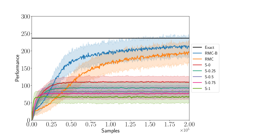
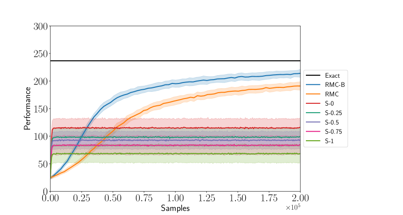
We compare the performance of RMC, RMC with biased gradient (denoted by RMC-B, see Remark 2), and actor critic with eligibility traces for the critic [3] (which we refer to as SARSA-λ𝜆\lambda and abbreviate as S-λ𝜆\lambda in the plots), with λ{0,0.25,0.5,0.75,1}𝜆00.250.50.751\lambda\in\{0,0.25,0.5,0.75,1\}. For both the RMC algorithms, we use the same runs to estimate the gradients (see Remark 2 in Sec. II). Each algorithm333For all algorithms, the learning rate is chosen using ADAM [33] with default hyper-parameters and the α𝛼\alpha parameter of ADAM equal to 0.050.050.05 for RMC, RMC-B, and the actor in SARSA-λ𝜆\lambda and the learning rate is equal to 0.10.10.1 for the critic in SARSA-λ𝜆\lambda. For RMC and RMC-B, the policy parameters are updated after N=5𝑁5N=5 renewals. is run 100100100 times and the mean and standard deviation of the performance (as estimated by the algorithms themselves) is shown in Fig. 1(a). The performance of the corresponding policy evaluated by Monte-Carlo evaluation over a horizon of 250250250 steps and averaged over 100100100 runs is shown in Fig. 1(b). The optimal performance computed using value iteration is also shown.

The results show that SARSA-λ𝜆\lambda learns faster (this is expected because the critic is keeping track of the entire value function) but has higher variance and gets stuck in a local minima. On the other hand, RMC and RMC-B learn slower but have a low bias and do not get stuck in a local minima. The same qualitative behavior was observed for other randomly generated models. Policy gradient algorithms only guarantee convergence to a local optimum. We are not sure why RMC and SARSA differ in which local minima they converge to. Also, it was observed that RMC-B (which is RMC with biased evaluation of the gradient) learns faster than RMC.
Refer to caption
(a)
Refer to caption
(b)
Figure 1: Performance of different learning algorithms on GARNET(100,10,50)GARNET1001050\text{GARNET}(100,10,50) with p=0.05𝑝0.05p=0.05 and γ=0.9𝛾0.9\gamma=0.9. (a) The performance estimated by the algorithms online. (b) The performance estimated by averaging over 100100100 Monte Carlo evaluations for a rollout horizon of 250250250. The solid lines show the mean value and the shaded region shows the ±plus-or-minus\pm one standard deviation region.

V-B Event-Triggered Communication

Refer to caption
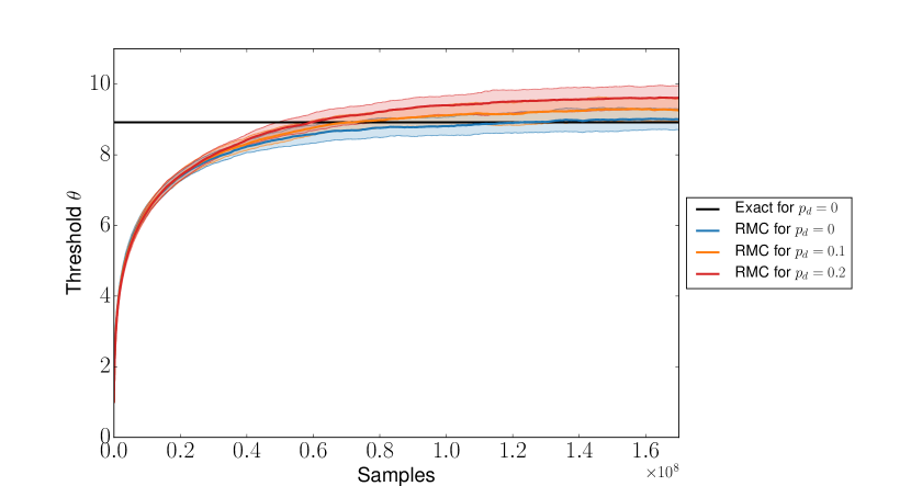
Figure 2: Policy parameters versus number of samples (sample values averaged over 100 runs) for event-driven communication using RMC for different values of pdsubscript𝑝𝑑p_{d}. The solid lines show the mean value and the shaded area shows the ±plus-or-minus\pm one standard deviation region.

In this experiment, we study an event-triggered communication problem that arises in networked control systems [34, 35]. A transmitter observes a first-order autoregressive process {Xt}t1subscriptsubscript𝑋𝑡𝑡1\{X_{t}\}_{t\geq 1}, i.e., Xt+1=αXt+Wtsubscript𝑋𝑡1𝛼subscript𝑋𝑡subscript𝑊𝑡X_{t+1}=\alpha X_{t}+W_{t}, where α,Xt,Wt𝛼subscript𝑋𝑡subscript𝑊𝑡\alpha,X_{t},W_{t}\in\mathbb{R}, and {Wt}t1subscriptsubscript𝑊𝑡𝑡1\{W_{t}\}_{t\geq 1} is an i.i.d. process. At each time, the transmitter uses an event-triggered policy (explained below) to determine whether to transmit or not (denoted by At=1subscript𝐴𝑡1A_{t}=1 and At=0subscript𝐴𝑡0A_{t}=0, respectively). Transmission takes place over an i.i.d. erasure channel with erasure probability pdsubscript𝑝𝑑p_{d}. Let Stsubscriptsuperscript𝑆𝑡S^{-}_{t} and St+subscriptsuperscript𝑆𝑡S^{+}_{t} denote the “error” between the source realization and it’s reconstruction at a receiver. It can be shown that Stsubscriptsuperscript𝑆𝑡S^{-}_{t} and St+subscriptsuperscript𝑆𝑡S^{+}_{t} evolve as follows [34, 35]: when At=0subscript𝐴𝑡0A_{t}=0, St+=Stsubscriptsuperscript𝑆𝑡subscriptsuperscript𝑆𝑡S^{+}_{t}=S^{-}_{t}; when At=1subscript𝐴𝑡1A_{t}=1, St+=0subscriptsuperscript𝑆𝑡0S^{+}_{t}=0 if the transmission is successful (w.p. (1pd)1subscript𝑝𝑑(1-p_{d})) and St+=Stsubscriptsuperscript𝑆𝑡subscriptsuperscript𝑆𝑡S^{+}_{t}=S^{-}_{t} if the transmission is not successful (w.p. pdsubscript𝑝𝑑p_{d}); and St+1=αSt++Wtsubscriptsuperscript𝑆𝑡1𝛼subscriptsuperscript𝑆𝑡subscript𝑊𝑡S^{-}_{t+1}=\alpha S^{+}_{t}+W_{t}. Note that this is a post-decision state model, where the post-decision state resets to zero after every successful transmission.444Had we used the standard MDP model instead of the post-decision state model, this restart would not have always resulted in a renewal.

The per-step cost has two components: a communication cost of λAt𝜆subscript𝐴𝑡\lambda A_{t}, where λ>0𝜆subscriptabsent0\lambda\in\mathbb{R}_{>0} and an estimation error (St+)2superscriptsubscriptsuperscript𝑆𝑡2(S^{+}_{t})^{2}. The objective is to minimize the expected discounted cost.

An event-triggered policy is a threshold policy that chooses At=1subscript𝐴𝑡1A_{t}=1 whenever |St|θsubscriptsuperscript𝑆𝑡𝜃|S^{-}_{t}|\geq\theta, where θ𝜃\theta is a design choice. Under certain conditions, such an event-triggered policy is known to be optimal [34, 35]. When the system model is known, algorithms to compute the optimal θ𝜃\theta are presented in [36, 37]. In this section, we use RMC to identify the optimal policy when the model parameters are not known.

In our experiment we consider an event-triggered model with α=1𝛼1\alpha=1, λ=500𝜆500\lambda=500, pd{0,0.1,0.2}subscript𝑝𝑑00.10.2p_{d}\in\{0,0.1,0.2\}, Wt𝒩(0,1)similar-tosubscript𝑊𝑡𝒩01W_{t}\sim{\cal N}(0,1), γ=0.9𝛾0.9\gamma=0.9, and use simultaneous perturbation variant of RMC555An event-triggered policy is a parametric policy but πθ(a|s)subscript𝜋𝜃conditional𝑎superscript𝑠\pi_{\theta}(a|s^{-}) is not differentiable in θ𝜃\theta. Therefore, the likelihood ratio method cannot be used to estimate performance gradient. to identify θ𝜃\theta. We run the algorithm 100 times and the result for different choices of pdsubscript𝑝𝑑p_{d} are shown in Fig. 2.666We choose the learning rate using ADAM with default hyper-parameters and the α𝛼\alpha parameter of ADAM equal to 0.01. We choose c=0.3𝑐0.3c=0.3, N=100𝑁100N=100 and Δ=𝒩(0,1)Δ𝒩01\Delta=\mathcal{N}(0,1) in Algorithm 2. For pd=0subscript𝑝𝑑0p_{d}=0, the optimal threshold computed using [37] is also shown. The results show that RMC converges relatively quickly and has low bias across multiple runs.

V-C Inventory Control

In this experiment, we study an inventory management problem that arises in operations research [38, 39]. Let StS_{t}\in\subset\mathbb{R} denote the volume of goods stored in a warehouse, At0subscript𝐴𝑡subscriptabsent0A_{t}\in\mathbb{R}_{\geq 0} denote the amount of goods ordered, and Dtsubscript𝐷𝑡D_{t} denotes the demand. The state evolves according to St+1=St+AtDt+1subscript𝑆𝑡1subscript𝑆𝑡subscript𝐴𝑡subscript𝐷𝑡1S_{t+1}=S_{t}+A_{t}-D_{t+1}.

We work with the normalized cost function:

C(s)=aps(1γ)/γ+ahs𝟙{s0}abs𝟙{s<0},𝐶𝑠subscript𝑎𝑝𝑠1𝛾𝛾subscript𝑎𝑠subscript1𝑠0subscript𝑎𝑏𝑠subscript1𝑠0C(s)=a_{p}s(1-\gamma)/\gamma+a_{h}s\mathds{1}_{\{s\geq 0\}}-a_{b}s\mathds{1}_{\{s<0\}},

where apsubscript𝑎𝑝a_{p} is the procurement cost, ahsubscript𝑎a_{h} is the holding cost, and absubscript𝑎𝑏a_{b} is the backlog cost (see [40, Chapter 13] for details).

It is known that there exists a threshold θ𝜃\theta such that the optimal policy is a base stock policy with threshold θ𝜃\theta (i.e., whenever the current stock level falls below θ𝜃\theta, one orders up to θ𝜃\theta). Furthermore, for sθ𝑠𝜃s\leq\theta, we have that [40, Sec 13.2]

Vθ(s)=C(s)+γ(1γ)𝔼[C(θD)].subscript𝑉𝜃𝑠𝐶𝑠𝛾1𝛾𝔼delimited-[]𝐶𝜃𝐷V_{\theta}(s)=C(s)+\frac{\gamma}{(1-\gamma)}\mathbb{E}[C(\theta-D)]. (22)

So, for Bρ(0,θ)superscript𝐵𝜌0𝜃B^{\rho}\subset(0,\theta), the value function is locally Lipschitz, with

Lθ=(ah+1γγap).subscript𝐿𝜃subscript𝑎1𝛾𝛾subscript𝑎𝑝L_{\theta}=\left(a_{h}+\frac{1-\gamma}{\gamma}a_{p}\right).

So, we can use approximate RMC to learn the optimal policy.

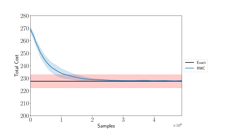
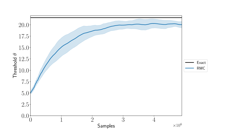
In our experiments, we consider an inventory management model with ah=1subscript𝑎1a_{h}=1, ab=1subscript𝑎𝑏1a_{b}=1, ap=1.5subscript𝑎𝑝1.5a_{p}=1.5, DtExp(λ)similar-tosubscript𝐷𝑡Exp𝜆D_{t}\sim\text{Exp}(\lambda) with λ=0.025𝜆0.025\lambda=0.025, start state s0=1subscript𝑠01s_{0}=1, discount factor γ=0.9𝛾0.9\gamma=0.9, and use simultaneous perturbation variant of approximate RMC to identify θ𝜃\theta. We run the algorithm 100100100 times and the result is shown in Fig. 3.777We choose the learning rate using ADAM with default hyper-parameters and the α𝛼\alpha parameter of ADAM equal to 0.25. We choose c=3.0𝑐3.0c=3.0, N=100𝑁100N=100, and Δ=𝒩(0,1)Δ𝒩01\Delta=\mathcal{N}(0,1) in Algorithm 2 and choose ρ=0.5𝜌0.5\rho=0.5 for approximate RMC. We bound the states within [100.0,100.0]100.0100.0[-100.0,100.0]. The optimal threshold and performance computed using [40, Sec 13.2]888For Exp(λ)Exp𝜆\text{Exp}(\lambda) demand, the optimal threshold is (see [40, Sec 13.2]) θ=1λlog(ah+abah+ap(1γ)/γ)).\theta^{*}=\frac{1}{\lambda}\log\left(\frac{a_{h}+a_{b}}{a_{h}+a_{p}(1-\gamma)/\gamma)}\right). is also shown. The result shows that RMC converges to an approximately optimal parameter value with total cost within the bound predicted in Theorem 2.
Refer to caption
(a)
Refer to caption
(b)
Figure 3: (a) Policy parameters and (b) Performance (total cost) versus number of samples (sample values averaged over 100 runs) for inventory control using RMC. The solid lines show the mean value and the shaded area shows the ±plus-or-minus\pm one standard deviation region. In (b), the performance is computed using (22) for the policy parameters given in (a). The red rectangular region shows the total cost bound given by Theorem 2.

VI Conclusions

We present a renewal theory based reinforcement learning algorithm called Renewal Monte Carlo. RMC retains the key advantages of Monte Carlo methods and has low bias, is simple and easy to implement, and works for models with continuous state and action spaces. In addition, due to the averaging over multiple renewals, RMC has low variance. We generalized the RMC algorithm to post-decision state models and also presented a variant that converges faster to an approximately optimal policy, where the renewal state is replaced by a renewal set. The error in using such an approximation is bounded by the size of the renewal set.

In certain models, one is interested in the peformance at a reference state that is not the start state. In such models, we can start with an arbitrary policy and ignore the trajectory until the reference state is visited for the first time and use RMC from that time onwards (assuming that the reference state is the new start state).

The results presented in this paper also apply to average reward models where the objective is to maximize

Jπ=limth1th𝔼Atπ(St)[t=0th1Rt|S0=s0].J_{\pi}=\lim_{t_{h}\to\infty}\frac{1}{t_{h}}\mathbb{E}_{A_{t}\sim\pi(S_{t})}\biggl{[}\sum_{t=0}^{t_{h}-1}R_{t}\biggm{|}S_{0}=s_{0}\biggr{]}. (23)

Let the stopping times τ(n)superscript𝜏𝑛\tau^{(n)} be defined as before. Define the total reward 𝖱(n)superscript𝖱𝑛\mathsf{R}^{(n)} and duration 𝖳(n)superscript𝖳𝑛\mathsf{T}^{(n)} of the n𝑛n-th regenerative cycle as

𝖱(n)=t=τ(n1)τ(n)1Rtand𝖳(n)=τ(n)τ(n1).formulae-sequencesuperscript𝖱𝑛subscriptsuperscriptsuperscript𝜏𝑛1𝑡superscript𝜏𝑛1subscript𝑅𝑡andsuperscript𝖳𝑛superscript𝜏𝑛superscript𝜏𝑛1\mathsf{R}^{(n)}=\smashoperator[r]{\sum_{t=\tau^{(n-1)}}^{\tau^{(n)}-1}}R_{t}\quad\text{and}\quad\mathsf{T}^{(n)}=\tau^{(n)}-\tau^{(n-1)}.

Let 𝖱θsubscript𝖱𝜃\mathsf{R}_{\theta} and 𝖳θsubscript𝖳𝜃\mathsf{T}_{\theta} denote the expected values of 𝖱(n)superscript𝖱𝑛\mathsf{R}^{(n)} and 𝖳(n)superscript𝖳𝑛\mathsf{T}^{(n)} under policy πθsubscript𝜋𝜃\pi_{\theta}. Then from standard renewal theory we have that the performance Jθsubscript𝐽𝜃J_{\theta} is equal to 𝖱θ/𝖳θsubscript𝖱𝜃subscript𝖳𝜃\mathsf{R}_{\theta}/\mathsf{T}_{\theta} and, therefore θJθ=Hθ/Tθ2subscript𝜃subscript𝐽𝜃subscript𝐻𝜃subscriptsuperscript𝑇2𝜃\nabla_{\theta}J_{\theta}=H_{\theta}/T^{2}_{\theta}, where Hθsubscript𝐻𝜃H_{\theta} is defined as in (9). We can use both variants of RMC prosented in Sec. II to obtain estimates of Hθsubscript𝐻𝜃H_{\theta} and use these to update the policy parameters using (10).

Acknowledgment

The authors are grateful to Joelle Pineau for useful feedback and for suggesting the idea of approximate RMC.

References

  • [1] D. Bertsekas and J. Tsitsiklis, Neuro-dynamic Programming, ser. Anthropological Field Studies.   Athena Scientific, 1996.
  • [2] L. P. Kaelbling, M. L. Littman, and A. W. Moore, “Reinforcement learning: A survey,” Journal of Artificial Intelligence Research, vol. 4, pp. 237–285, 1996.
  • [3] R. S. Sutton and A. G. Barto, Reinforcement learning: An introduction.   MIT Press, 1998.
  • [4] C. Szepesvári, Algorithms for reinforcement learning.   Morgan & Claypool Publishers, 2010.
  • [5] R. S. Sutton, D. A. McAllester, S. P. Singh, and Y. Mansour, “Policy gradient methods for reinforcement learning with function approximation,” in Advances in Neural Information Processing Systems, Nov. 2000, pp. 1057–1063.
  • [6] S. M. Kakade, “A natural policy gradient,” in Advances in Neural Information Processing Systems, Dec. 2002, pp. 1531–1538.
  • [7] V. R. Konda and J. N. Tsitsiklis, “On actor-critic algorithms,” SIAM Journal on Control and Optimization, vol. 42, no. 4, pp. 1143–1166, 2003.
  • [8] J. Schulman, S. Levine, P. Abbeel, M. Jordan, and P. Moritz, “Trust region policy optimization,” in Proceedings of the 32nd International Conference on Machine Learning (ICML-15), June 2015, pp. 1889–1897.
  • [9] J. Schulman, F. Wolski, P. Dhariwal, A. Radford, and O. Klimov, “Proximal policy optimization algorithms,” arXiv preprint arXiv:1707.06347, 2017.
  • [10] D. Silver, J. Schrittwieser, K. Simonyan, I. Antonoglou, A. Huang, A. Guez, T. Hubert, L. Baker, M. Lai, A. Bolton, Y. others Chen, T. Lillicrap, F. Hui, L. Sifre, G. van den Driessche, T. Graepel, and D. Hassabis, “Mastering the game of go without human knowledge,” Nature, vol. 550, no. 7676, p. 354, 2017.
  • [11] P. Glynn, “Optimization of stochastic systems,” in Proc. Winter Simulation Conference, Dec. 1986, pp. 52–59.
  • [12] ——, “Likelihood ratio gradient estimation for stochastic systems,” Communications of the ACM, vol. 33, pp. 75–84, 1990.
  • [13] P. Marbach and J. N. Tsitsiklis, “Simulation-based optimization of Markov reward processes,” IEEE Trans. Autom. Control, vol. 46, no. 2, pp. 191–209, Feb 2001.
  • [14] ——, “Approximate gradient methods in policy-space optimization of Markov reward processes,,” Discrete Event Dynamical Systems, vol. 13, no. 2, pp. 111–148, 2003.
  • [15] O. Hernández-Lerma and J. B. Lasserre, Discrete-time Markov Control Processes: Basic Optimality Criteria.   Springer Science & Business Media, 1996, vol. 30.
  • [16] V. Borkar, Stochastic Approximation: A Dynamical Systems Viewpoint.   Cambridge University Press, 2008.
  • [17] W. Feller, An Introduction to Probability Theory and its Applications.   John Wiley and Sons, 1966, vol. 1.
  • [18] R. Y. Rubinstein, “Sensitivity analysis and performance extrapolation for computer simulation models,” Operations Research, vol. 37, no. 1, pp. 72–81, 1989.
  • [19] R. J. Williams, “Simple statistical gradient-following algorithms for connectionist reinforcement learning,” Machine learning, vol. 8, no. 3-4, pp. 229–256, 1992.
  • [20] E. Greensmith, P. L. Bartlett, and J. Baxter, “Variance reduction techniques for gradient estimates in reinforcement learning,” Journal of Machine Learning Research, vol. 5, no. Nov, pp. 1471–1530, 2004.
  • [21] J. Peters and S. Schaal, “Policy gradient methods for robotics,” in International Conference on Intelligent Robots and Systems, 2006 IEEE/RSJ.   IEEE, Oct. 2006, pp. 2219–2225.
  • [22] P. Thomas, “Bias in natural actor-critic algorithms,” in International Conference on Machine Learning, June 2014, pp. 441–448.
  • [23] J. C. Spall, “Multivariate stochastic approximation using a simultaneous perturbation gradient approximation,” IEEE Trans. Autom. Control, vol. 37, no. 3, pp. 332–341, 1992.
  • [24] J. L. Maryak and D. C. Chin, “Global random optimization by simultaneous perturbation stochastic approximation,” IEEE Trans. Autom. Control, vol. 53, no. 3, pp. 780–783, Apr. 2008.
  • [25] V. Katkovnik and Y. Kulchitsky, “Convergence of a class of random search algorithms.” Automation and Remote Control, vol. 33, no. 8, pp. 1321–1326, 1972.
  • [26] S. Bhatnagar, H. Prasad, and L. Prashanth, Stochastic Recursive Algorithms for Optimization: Simultaneous Perturbation Methods.   Springer, 2013, vol. 434.
  • [27] B. Van Roy, D. P. Bertsekas, Y. Lee, and J. N. Tsitsiklis, “A neuro-dynamic programming approach to retailer inventory management,” in 36th IEEE Conference on Decision and Control, 1997, vol. 4, Dec. 1997, pp. 4052–4057.
  • [28] W. B. Powell, Approximate Dynamic Programming: Solving the Curses of Dimensionality, 2nd ed.   John Wiley & Sons, 2011.
  • [29] K. Hinderer, “Lipschitz continuity of value functions in Markovian decision processes,” Mathematical Methods of Operations Research, vol. 62, no. 1, pp. 3–22, Sep 2005.
  • [30] E. Rachelson and M. G. Lagoudakis, “On the locality of action domination in sequential decision making,” in 11th International Symposium on Artificial Intelligence and Mathematics (ISIAM 2010), Fort Lauderdale, US, Jan. 2010, pp. pp. 1–8.
  • [31] M. Pirotta, M. Restelli, and L. Bascetta, “Policy gradient in Lipschitz Markov decision processes,” Machine Learning, vol. 100, no. 2, pp. 255–283, Sep 2015.
  • [32] S. Bhatnagar, R. Sutton, M. Ghavamzadeh, and M. Lee, “Natural actor-critic algorithms,” Department of Computing Science, University of Alberta, Canada, Tech. Rep., 2009.
  • [33] D. Kingma and J. Ba, “Adam: A method for stochastic optimization,” arXiv preprint arXiv:1412.6980, 2014.
  • [34] G. M. Lipsa and N. Martins, “Remote state estimation with communication costs for first-order LTI systems,” IEEE Trans. Autom. Control, vol. 56, no. 9, pp. 2013–2025, Sep. 2011.
  • [35] J. Chakravorty, J. Subramanian, and A. Mahajan, “Stochastic approximation based methods for computing the optimal thresholds in remote-state estimation with packet drops,” in Proc. American Control Conference, Seattle, WA, May 2017, pp. 462–467.
  • [36] Y. Xu and J. P. Hespanha, “Optimal communication logics in networked control systems,” in 43rd IEEE Conference on Decision and Control, Dec. 2004, pp. 3527–3532.
  • [37] J. Chakravorty and A. Mahajan, “Fundamental limits of remote estimation of Markov processes under communication constraints,” IEEE Trans. Autom. Control, vol. 62, no. 3, pp. 1109–1124, Mar. 2017.
  • [38] K. J. Arrow, T. Harris, and J. Marschak, “Optimal inventory policy,” Econometrica: Journal of the Econometric Society, pp. 250–272, 1951.
  • [39] R. Bellman, I. Glicksberg, and O. Gross, “On the optimal inventory equation,” Management Science, vol. 2, no. 1, pp. 83–104, 1955.
  • [40] P. Whittle, Optimization Over Time: Dynamic Programming and Optimal Control.   John Wiley and Sons, Ltd., 1982.