An Iwasawa-Taniguchi Effect for Compton-thick Active Galactic Nuclei

Abstract

We present the first study of an Iwasawa-Taniguchi/‘X-ray Baldwin’ effect for Compton-thick active galactic nuclei (AGN). We report a statistically significant anti-correlation between the rest-frame equivalent width (EW) of the narrow core of the neutral Fe K$\alpha$ fluorescence emission line, ubiquitously observed in the reflection spectra of obscured AGN, and the mid-infrared $12\,\mu\rm m$ continuum luminosity (taken as a proxy for the bolometric AGN luminosity). Our sample consists of 72 Compton-thick AGN selected from pointed and deep-field observations covering a redshift range of $z\sim 0.0014-3.7$. We employ a Monte Carlo-based fitting method, which returns a Spearman’s Rank correlation coefficient of $\rho\,=\,-0.28\pm 0.12$, significant to 98.7% confidence. The best fit found is $\mathrm{log}(\mathrm{EW}_{\mathrm{Fe\,K}\alpha})\,\propto\,-0.08\pm 0.04\,\mathrm{log}(L_{12\,\rm{\mu}\rm m})$, which is consistent with multiple studies of the X-ray Baldwin effect for unobscured and mildly obscured AGN. This is an unexpected result, as the Fe K$\alpha$ line is conventionally thought to originate from the same region as the underlying reflection continuum, which together constitute the reflection spectrum. We discuss the implications this could have if confirmed on larger samples, including a systematic underestimation of the line of sight X-ray obscuring column density and hence the intrinsic luminosities and growth rates for the most luminous AGN.

1 Introduction

X-ray continuum emission from active galactic nuclei (AGN) typically takes the form of a broadband powerlaw with a high-energy cut-off around 300 keV (Ballantyne14; Malizia14), and originates from Comptonization of ultraviolet accretion disc photons in a hot X-ray corona (Haardt91; Haardt93). Line of sight opacity alters this emission via photoelectric absorption and Compton scattering. If properly accounted for, this can be used to predict the intrinsic spectral energy distribution of an AGN and thus indirectly study the circumnuclear environment of AGN. Many studies have revealed that the vast majority of AGN are intrinsically obscured with hydrogen column densities ($N_{\rm H}$) greater than the Galactic value (Risaliti99b; Burlon11; Ricci15, $N_{\rm H}\gtrsim 10^{22}\,\rm{cm}^{-2}$). For $N_{\rm H}\lesssim 10^{24}\,\rm{cm}^{-2}$, the intrinsic power law typically dominates over any other spectral features in the X-ray band. As the column increases to $N_{\rm H}>1.5\times 10^{24}\,\rm{cm}^{-2}$, the obscuring material becomes optically thick in X-rays to Compton scattering, in the Compton-thick regime. Here, the soft X-ray (E $\lesssim 10$ keV) spectrum is depleted and flattened due to the interplay of photoelectric absorption and Compton downscattering. Depending on the orientation, geometry and column of the Compton-thick obscurer, the hard X-ray spectrum (E$\,\gtrsim 10\,\rm{keV}$) can either be dominated by the direct intrinsic powerlaw component, absorbed along the line of sight (transmission-dominated Compton-thick AGN); or by a Compton-scattered reflection component, from intrinsic flux reprocessed by the obscurer into the line of sight (reflection-dominated Compton-thick AGN).

The geometrical configuration of the X-ray obscuring and reprocessing medium is typically assumed to be roughly axissymmetric but anisotropic (Murphy09; Ikeda09; Brightman11b; Balokovic18). This is analogous to the putative torus in the Unified Model of AGN (Antonucci93; Urry95; Netzer15) invoked to explain the infrared and optical emission observed from different classes of AGN as intrinsically a single class observed at different orientation angles. The X-ray obscurer in Compton-thick AGN is what defines the spectral shape of the reprocessed reflection spectrum, which typically features two key components (Lightman88; Reynolds99):

1. A narrow Fe K$\rm{\alpha}$ fluorescence emission line arising from neutral (and hence cold) iron, with a characteristic energy of 6.4 keV in the rest frame of the source. This emission line is typically the most prominent in the X-ray spectra of AGN, due to a combination of the fluorescence yield and relative abundances of the gas located within the torus.

2. An underlying (flat) Compton scattered continuum with a broad ‘Compton hump’ peaking at $\sim 30\,\rm{keV}$ formed from the combination of photoelectric absorption at E $\lesssim 10\,\rm{keV}$ and Compton downscattering from higher energies.

Modelling the strength and shape of the neutral Fe K$\rm{\alpha}$ fluorescence line together with the Compton hump can yield the line of sight obscuring column to a source. This requires an observed X-ray spectrum spanning the Compton hump at $\sim 30\,\rm{keV}$ and the soft X-ray emission $\lesssim 10\,\rm{keV}$, to provide constraints on the continuum and reflection components. However, many previous X-ray observations of AGN have typically been restricted to the E $\lesssim 10\,\rm{keV}$ energy region (Suzaku XIS, Chandra, XMM-Newton), completely missing the Compton hump for local sources. This typically means that any attempt to fit AGN X-ray spectra in this energy region with the objective of constraining the line of sight $N_{\rm H}$ depends heavily on the Fe K$\rm{\alpha}$ fluorescence line alone, and can be uncertain.

Despite being an indicator of high obscuring columns, the equivalent width (EW) of the narrow core of the neutral Fe K$\alpha$ fluorescence line has been observed to anti-correlate with the underlying intrinsic X-ray continuum luminosity in samples of transmission-dominated AGN. This effect was first reported by Iwasawa93 for a sample of 37 largely unobscured AGN, observed by the Ginga satellite. The best fit linear relation derived was of the form $\rm{log(EW}_{\rm{Fe\,K}\alpha})\,\propto\,-0.20\pm 0.03\,\mathrm{log}(L_{2-10\,\rm{keV}})$. This is sometimes referred to as the ‘X-ray Baldwin’ effect due to the similarity with the study by Baldwin77 on the anti-correlation between the EW of the $\rm{C}\,\textsc{iv}\,1549\,\AA$ ultraviolet emission line and AGN continuum. Here we refer to the X-ray Baldwin effect as the ‘Iwasawa-Taniguchi’ effect.

The Iwasawa-Taniguchi effect has been explored in further detail for different AGN classes. For example, Page04 reported an Iwasawa-Taniguchi effect of $\mathrm{log}(\mathrm{EW}_{\mathrm{Fe\,K}\alpha})\,\propto\,-0.17\pm 0.08\,\mathrm{log}(L_{2-10\,\rm{keV}})$ for a sample of 53 type 1 AGN observed by XMM-Newton, with the slope being consistent with that of Iwasawa93. However, Jiang06 later reported a much shallower anti-correlation of $\mathrm{log}(\mathrm{EW}_{\mathrm{Fe\,K}\alpha})\,\propto\,-0.10\pm 0.05\,\mathrm{log}(L_{2-10\,\rm{keV}})$ for a sample of 75 radio-quiet AGN observed by XMM-Newton and Chandra. The authors attribute the reduction in slope of the anti-correlation to radio-loud contamination of previous AGN samples, proposing that radio-loud AGN could have an enhanced continuum contribution from a relativistic jet. The authors further postulated that short-term variability of the primary X-ray source could, in part, contribute to the anti-correlation. Despite the shallower gradient found, two measurements of the same gradient would be expected to differ by the separation between Iwasawa93 and Jiang06 $\sim 8$% of the time, and are thus not strongly inconsistent with each other. Bianchi07 later studied the Iwasawa-Taniguchi effect for a sample of 157 radio-quiet unobscured type 1 AGN, including narrow line Seyfert 1s (which share some spectral characteristics with obscured AGN). In contrast to Jiang06, the authors found a somewhat steeper anti-correlation of $\mathrm{log}(\mathrm{EW}_{\mathrm{Fe\,K}\alpha})\,\propto\,-0.17\pm 0.03\,\mathrm{log}(L_{2-10\,\rm{keV}})$, fully consistent with the original Iwasawa-Taniguchi effect and Page04. Bianchi07 further suggest an additional strong anti-correlation between the Fe K$\rm{\alpha}$ fluorescence line EW and Eddington ratio. Indeed, Ricci13b tested the positive relation between the photon index and Eddington ratio found for AGN (Lu99; Shemmer06; Risaliti09; Brightman13; Trakhtenbrot17), even into the Compton-thick regime (Brightman16), finding that this could contribute to the Iwasawa-Taniguchi effect. This is because a lower Eddington ratio (and thus photon index, resulting in a flatter spectrum) would lead to more photons at the energy required to generate iron K$\alpha$ fluorescence, giving a larger EW.

Individual source variability has been shown to considerably affect the strength of the anti-correlation, with Shu12 finding a reduction in the observed slope from $\mathrm{log}(\mathrm{EW}_{\mathrm{Fe\,K}\alpha})\,\propto\,-0.22\,\mathrm{log}(L_{2-10\,\rm{keV}})$ to $\mathrm{log}(\mathrm{EW}_{\mathrm{Fe\,K}\alpha})\,\propto\,-0.13\,\mathrm{log}(L_{2-10\,\rm{keV}})$, after accounting for the time-averaged Fe K$\rm{\alpha}$ strength in a sample of 32 AGN with $N_{\rm H}\lesssim 10^{23}\,\rm{cm}^{-2}$, observed multiple times by the Chandra high-energy grating (HEG).

The conventional Iwasawa-Taniguchi effect describes the strength of the Fe K$\rm{\alpha}$ line relative to the intrinsic continuum (readily available for unobscured AGN), but a difficulty is introduced when trying to study the effect for obscured sources, which by definition start to lack a prominent transmitted intrinsic component in the iron line flux, to measure the EW against. Ricci14 report a significant detection of the Iwasawa-Taniguchi effect for two separate samples of Seyfert 1s and 2s, consistently of $\mathrm{log}(L_{\mathrm{Fe\,K}\alpha}/L_{\rm{10-50\,keV}})\,\propto\,-0.11\pm 0.01\,\mathrm{log}(L_{10-50\,\rm{keV}})$. Type 2 Seyferts are typically observed to be obscured in the optical and often X-rays also (e.g., Koss17). Thus the work of Ricci14 was the first study into the effect for obscured sources, in which the higher $10-50\,\rm{keV}$ energy range was used to describe the intrinsic continuum and Fe K$\alpha$ EW since photoelectric absorption is minimised for photons at harder energies. Interestingly, the authors postulate that the consistency of slopes between Seyfert 1s and 2s could indicate that the physical mechanism responsible for the Iwasawa-Taniguchi effect is unaffected by orientation under Unification schemes. For a breakdown of the results into the Iwasawa-Taniguchi effect from the different works mentioned above, see Table 1 of Ricci13a.

Numerous physical scenarios have been considered to explain the observed Iwasawa-Taniguchi effect, with one of the most favoured being an intrinsic luminosity-dependent covering factor of neutral obscuring gas surrounding the AGN. This effect was first suggested in Lawrence82 & Lawrence91, dubbed the ‘receding torus’, and has been observed in various large AGN samples. This idea is strengthened by the results from multiple studies reporting an increased number density of obscured AGN at lower X-ray luminosities (Ueda11; Lusso13; Merloni14; Georgakakis17). Simulations of torus reprocessing of X-ray emission have also shown that the Fe K$\alpha$ line EW can be dramatically enhanced when the observer is exposed to less intrinsic flux than the reprocessor (Krolik94), which is physically attained with higher covering factors of the central engine.

A receding torus model provides a possible explanation for the Iwasawa-Taniguchi effect in which the observed spectrum contains a dominant unscattered component, as is the case for transmission-dominated obscured systems. The prominence of the direct transmitted component would scale with intrinsic luminosity, resulting in the narrow Fe K$\alpha$ line (arising from the reflection component) being diminished by the brightened intrinsic power law. To illustrate the contribution to the observed flux from the transmitted component vs. the reflected component from an anisotropic X-ray reprocessor, Figure 1 shows the relative contribution to the total line flux (approximated here to $6-7.9\,$keV) from the transmitted component (blue) and reflected component (red). This was simulated with the borus02_v170709a (borus02) model (Balokovic18), in which the obscurer is spherically distributed with polar cutouts. For each column density, we plot the average flux ratio for a series of covering factor/inclination angle combinations, and sources are predicted to become reflection-dominated in the Fe K$\alpha$ line for $\rm{log}\,\textit{N}_{\rm H}\,\gtrsim\,23.6\,\rm{cm}^{-2}$.

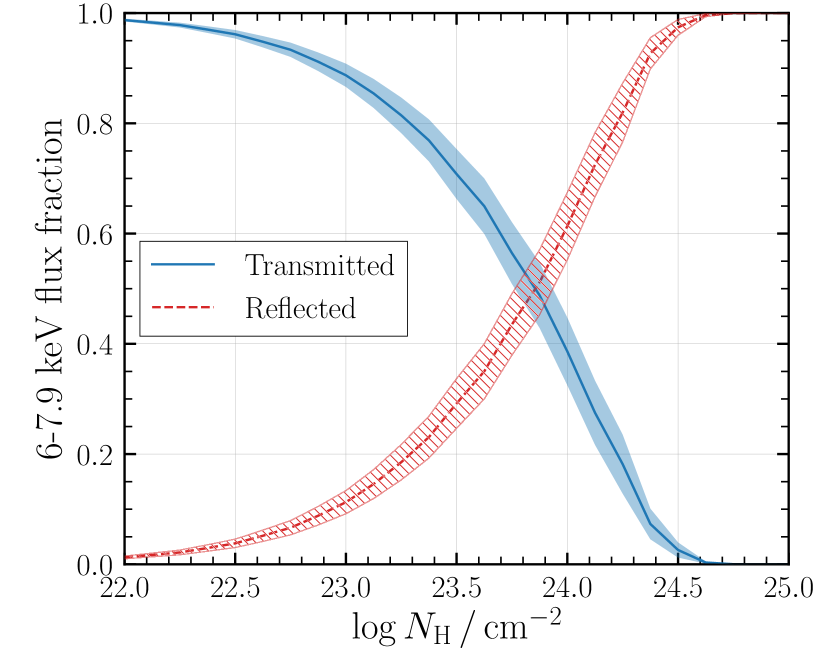
Figure 1: The contribution to the total observed flux in the iron line region (approximated to $6-7.9\,$keV) from the direct transmitted component (blue) and Compton-scattered reflected component (red). This was simulated using the borus02 X-ray reprocessor model (Balokovic18), for a spherically distributed obscurer with polar cutouts. For each column density, the average flux ratio for a series of covering factor/inclination angle combinations is plotted with the confidence region showing the range between the minimum and maximum found around the average.

Recent dedicated studies into specific X-ray-obscured AGN appear to show a trend of decreased neutral Fe K$\rm{\alpha}$ line EW, with increasing luminosity. Here we highlight three Compton-thick case studies for comparison; also illustrated in Figure 2:

1. Local low luminosity Compton-thick Seyferts typically show prominent lines. One of the strongest observed Fe K$\rm{\alpha}$ line EWs found to date was for IC 3639 (Boorman16); a reflection-dominated Compton-thick AGN with infrared bolometric luminosity (in the $8-1000\,\rm{\mu}\rm{m}$ wavelength range) of $\mathrm{log}(L_{8-1000\,\rm{\mu m}}\,[L_{\odot}])\sim 10.9$ and $\mathrm{EW}_{\mathrm{Fe\,K}\alpha}\sim 3\,\rm{keV}$, relative to the observed underlying reflection continuum.

2. On the other hand, NGC 7674 (Gandhi17) is a heavily Compton-thick Seyfert 2, with a higher infrared bolometric luminosity of $\mathrm{log}(L_{8-1000\,\rm{\mu m}}\,[L_{\odot}])\sim 11.6$. Yet the source has an observed EW of the neutral line of $\mathrm{EW}_{\mathrm{Fe\,K}\alpha}\sim 0.4\,\rm{keV}$: the lowest constrained EW of the Fe K$\alpha$ line detected for any bona-fide Compton-thick AGN to date.

3. At the highest luminosities, Gilli11; Gilli14 is the most distant ($z\sim 4.75$) Compton-thick AGN classified to date, with infrared bolometric luminosity $\mathrm{log}(L_{8-1000\,\rm{\mu m}}\,[L_{\odot}])\sim 12.8$. Interestingly, the neutral Fe K$\rm{\alpha}$ fluorescence line is not detected in the observed X-ray spectrum obtained from the 4 Ms Chandra Deep Field South observation, yet with a prominent ionised Hydrogen-like iron line at $\sim 6.9\,$keV to $\sim 2\,\sigma$ confidence, with rest-frame EW = $2.8^{+1.7}_{-1.4}\,$keV. In fact, there is increasing observational evidence for prominent ionised iron lines in luminous infrared galaxies (LIRGs: $\mathrm{log}(L_{8-1000\,\rm{\mu m}}\,[L_{\odot}])>11$) (Iwasawa09).

We note that although the contribution to the infrared flux from star formation will increase with bolometric flux, the AGN contribution also increases. This means a higher infrared flux should indicate a more intrinsically luminous AGN. These three case study sources are illustrated in Figure 2, in which we plot the data/model ratio for each source after fitting a powerlaw to the observed spectrum. Although NGC 7674 appears to show a large component to the observed flux around $6-6.5\,$keV, the narrow core of the neutral Fe K$\rm{\alpha}$ line is considerably weaker. The panels have been binned for clarity.

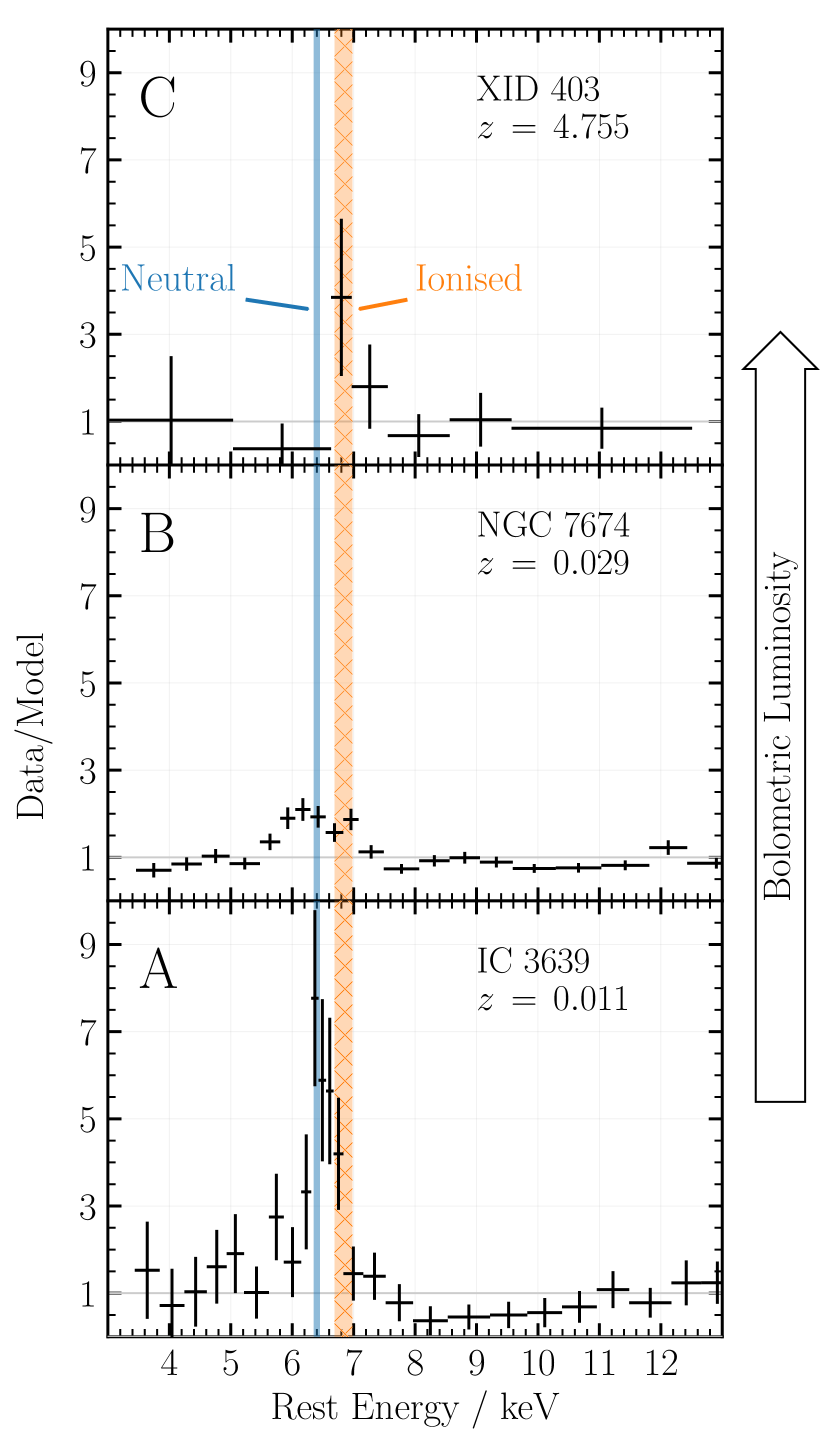
Figure 2: Three Compton-thick case studies illustrating the motivation for the studying a Compton-thick Iwasawa-Taniguchi effect. Panel A: IC 3639 (Boorman16): a local Compton-thick AGN at $z\,=\,0.011$ with bolometric infrared luminosity, $\mathrm{log}(L_{8-1000\,\rm{\mu m}}\,[L_{\odot}])\sim 10.9$, and one of the strongest neutral Fe K$\alpha$ lines reported in the literature. Panel B: NGC 7674 (Gandhi17): a local Compton-thick AGN, and luminous infrared galaxy with bolometric infrared luminosity, $\mathrm{log}(L_{8-1000\,\rm{\mu m}}\,[L_{\odot}])\sim 11.6$. Contrastingly, this source has the lowest neutral Fe K$\alpha$ EW reported for local Compton-thick AGN. Furthermore, the spectrum clearly shows a contribution to the residuals in the ionised energy region. Panel C: LESS J033229.4-275619 (Gilli14): the highest redshift Compton-thick AGN currently known, with $\mathrm{log}(L_{8-1000\,\rm{\mu m}}\,[L_{\odot}])\sim 12.8$. The spectrum plotted is from a 7 Ms observation of Chandra Deep Field South (CDFS). The neutral emission is not detected, yet a considerable flux contribution can be seen in the ionised emission line energy region. Each source was fitted with a redshifted powerlaw in xspec, and the resulting data/model ratio is shown. For all panels, the narrow core of the neutral line is shown with the orange region for $E=6.35-6.45$ keV, and the ionised line region is shown in blue hatch for the $E=6.69-6.98$ keV region (to encompass the 6.7 and 6.97 keV ionised lines).

This paper presents the first study into an Iwasawa-Taniguchi effect for Compton-thick AGN, with Fe K$\rm{\alpha}$ EWs measured relative to the observed continuum vs. rest-frame mid-infrared $12\,\rm{\mu}\rm m$ luminosity ($L_{\rm{12\,\mu m}}$; taken as a proxy for the intrinsic AGN bolometric luminosity). The cosmology adopted for computing luminosity distances is $H_{0}$ = 67.3 km s^-1 Mpc^-1, ${\rm\Omega}_{\Lambda}$ = 0.685 and ${\rm\Omega}_{\rm M}$ = 0.315 (Planck14) The paper is organised as follows: Section 2 describes our source selection and the sample used in our statistical analysis. Section 3 then describes our method for clarifying candidate Compton-thick AGN, as well as for determining the $L_{\rm{12\,\mu m}}$ and Fe K$\rm{\alpha}$ EW values. We then discuss our fitting procedure. Section 4 comprises our main results, followed by the discussion and implications of the effect if confirmed on future larger Compton-thick AGN samples, in Section LABEL:sec:discussion. We summarise our findings in Section LABEL:sec:summary.

2 THE SAMPLE

Our primary goal whilst collating Compton-thick candidates from the literature was to cover a broad redshift (and hence luminosity) range. Furthermore, X-ray spectra encompassing the observed frame neutral Fe K$\rm{\alpha}$ fluorescence line, seen at $6.4/(1+z)\,\rm{keV}$ in the rest-frame, were required. In order to robustly quantify the EW required a detection of the underlying observed continuum, neighbouring the line centroid. Below we include details of the high and low redshift subsamples we include in our work.

2.1 High redshift

For higher redshift (or fainter) sources, Chandra observations were ideal due to low background and optimal sensitivities in the $0.5-8.0\,\rm{keV}$ energy range. At high redshift, the k-corrected Compton hump also shifts to the observed Chandra energy range. A considerable contribution to our sample thus includes the Brightman14 compilation of Compton-thick AGN candidates collated from archival deep Chandra surveys. The original sample includes $\sim$ 100 Compton-thick candidates. A source was only retained for our study if it met the following criteria:

1. $>50$ total X-ray counts detected in the Chandra energy band.

2. A spectroscopic redshift.

3. A line of sight column density of $N_{\rm H}\geq 1.5\times 10^{24}\,\rm{cm}^{-2}$ at 90% confidence, determined by Brightman14.

4. Infrared detection by the Wide-field Infrared Survey Explorer (WISE) or Spitzer Space Telescope to enable a reliable $L_{\rm{12\,\mu m}}$ estimate.

Of the resulting candidates, a further two were excluded due to a disagreement with our Compton-thick classification (COSMOS 0661 & COSMOS 1517: Section 3), leaving a total of 27 sources from Brightman14. An additional five high redshift sources come from further Compton-thick studies by Feruglio11; Corral16, Georgantopoulos13, Lanzuisi15 and Hlavacek-Larrondo17. In total, 32 sources make up our high redshift subsample of Compton-thick candidates.

2.2 Low redshift

A major contribution to our low redshift subsample comes from Ricci15. The sample consists of 55 Compton-thick AGN candidates selected from the Neil Gehrels Swift/Burst Alert Telescope (BAT) 70-month catalogue, all within the local Universe (average $z=0.055$). Of these 55, we rejected 19 sources without publicly available NuSTAR observations. NuSTAR (Harrison13) is the first true hard X-ray imaging instrument in the $3-79\,\rm{keV}$ energy range, encompassing the full underlying reflection continuum for low redshift AGN, and thus ideal for studying Compton-thick candidates. By combining with soft X-ray observations, many works have constrained the $N_{\rm H}$ values for numerous obscured, Compton-thick and changing-look AGN to date (e.g. Arevalo14, Circinus Galaxy; Balokovic14, NGC 424, NGC 1320, IC 2560; Gandhi14, Mrk 34; Teng14, Mrk 231; Annuar15, NGC 5643; Bauer15, NGC 1068; Ptak15, Arp 299; Boorman16, IC 3639; Megamaser sample; Masini16a, Mrk 1210; Ricci16, IC 751; Ricci17a, WISE J1036 +0449; Annuar17, NGC 1448; Gandhi17, NGC 7674), hence our preference for NuSTAR availability.

An additional three sources from the Ricci15 sample were excluded due to a disagreement with our mid-infrared diagnostic Compton-thick classification (2MASX J09235371-3141305; MCG -02-12-017; NGC 6232, Section 3).

The last contribution to our low redshift subsample comes from the Gandhi14 compilation of bona-fide Compton-thick AGN, updated to include IC 3639 (Boorman16), NGC 1448 (Annuar17) and NGC 7674 (Gandhi17), whilst excluding changing-look candidates: Mrk 3 (Ricci15, find a Compton-thin column density to 90% confidence), NGC 4102, NGC 4939, NGC 4785 (Gandhi15a; Marchesi17) and NGC 7582 (Rivers15). In total, 40 sources make up our low redshift subsample of Compton-thick candidates. Full details of the 72 (low + high redshift) Compton-thick candidates in our sample are included in Table LABEL:tab:sample.

3 METHOD

3.1 Infrared luminosities

In selecting a suitable proxy for the bolometric luminosity of each source, we adhered to the following criteria: (1) the bolometric luminosity could not be derived from the spectral energy region responsible for the neutral Fe K$\rm{\alpha}$ line nor from the continuum surrounding the line that would be used to derive an EW, and (2) the proxy should be prominent and well detected for Compton-thick AGN.

We used the infrared contribution to the broadband spectra of our AGN sample, which is considered to have sizeable contributions in this wavelength range due to reprocessing of the primary intrinsic AGN emission. Since typical AGN contributions to composite galaxy spectra dominate at $\sim 6-20\,\mu\rm m$ (Mullaney11), we used the rest-frame $12\,\rm{\mu}\rm m$ luminosity of each source.

To determine the rest-frame $12\,\mu\rm m$ luminosity, we utilised the infrared spectral template of Mullaney11 to interpolate the rest-frame $12\,\mu\rm m$ flux from observed-frame flux measurements as close to $12\,\mu\rm m$ as possible. For high-quality infrared observations, we use the WISE and Spitzer Multiband Imaging Photometer (MIPS). WISE had four imaging channels onboard (W1, W2, W3 & W4) corresponding to $\lambda=3.35\,\mu\rm m,\,4.60\,\mu\rm m,\,11.56\,\mu\rm m,\,22.09\,\mu\rm m$, respectively (Wright10), whereas Spitzer/MIPS was capable of imaging in spectral bands centered on $\lambda=\,24\,\mu\rm m,\,70\,\mu\rm m,\,160\,\mu\rm m$. For $z\lesssim 0.84$ a robust interpolation could be made from W3 and W4 observations. However, for higher redshift sources in which the k-correction shifts the rest-frame $12\,\mu\rm m$ luminosity to wavelengths beyond W4 (or for poorly constrained/faint observations from WISE), we use Spitzer/MIPS.

For archival WISE observations, we use the AllWISE Source Catalog to get profile-fitted magnitudes and the NASA Extragalactic Database (NED) to search for archival Spitzer/MIPS observations.

To test how representative the Mullaney11 template was for predicting the 12 $\mu$m luminosity for the AGN in our sample with $L_{2\,-\,10\,\rm{keV}}<10^{42}\,\rm{erg\,s}^{-1}$ or $L_{2\,-\,10\,\rm{keV}}>10^{44}\,\rm{erg\,s}^{-1}$, we compared the interpolated luminosities with those predicted from the type 2 AGN template from Polletta07, which were derived over a wider range of luminosities. On average, the offset between the interpolated luminosities from the two templates was only $\sim 0.06$ dex.

3.2 Compton-thick confirmation of sample

Strong correlations between mid-infrared and intrinsic X-ray emission have been found with ground-based high angular resolution observations of AGN, around $12\,\mu\rm m$ (Horst08; Levenson09; Gandhi09; Asmus15). A similar correlation has been found as a function of large aperture $6\,\mu\rm m$ luminosity, with akin results (Lutz04; Mateos15; Stern15; Chen17), and at 5.8 $\mu$m (Lanzuisi09). The $12\,\mu\rm m$ luminosity correlation has been used with considerable success for identifying candidate Compton-thick AGN. Correcting X-ray absorption in Compton-thick sources acts to increase the observed X-ray luminosity to values consistent with the relation. We refer the reader to Boorman16 for the effects of absorption correction on X-ray luminosities relative to their observed mid-infrared luminosities for the Gandhi14 compilation of bona fide Compton-thick AGN. Here we use the study of the X-ray vs. $12\,\mu\rm m$ correlation reported in Asmus15 to classify our sample as candidate Compton-thick.

The rest-frame observed (i.e. absorbed) $2-10\,\rm{keV}$ luminosity was computed from a fit to the available X-ray spectra within xspec (for objects without a reported observed X-ray flux), and plotted against the rest-frame $12\,\mu\rm m$ luminosity, interpolated from the Mullaney11 AGN spectral template. These observed fluxes are plotted in Figure 3 (grey points), with a 30% and 15% uncertainty on the X-ray and $12\,\mu\rm m$ luminosities, respectively. The original correlation found by Asmus15 is shown with a solid (green) line for clarity, together with the 1-$\sigma$ scatter. On average, the sample displays a mean ratio of observed X-ray to mid-infrared flux of $-2.0\pm 0.7$ dex, and this is shown over plotted with a dashed (grey) line and shading. An average deviation of greater than two orders of magnitude from the relation is indicative of Compton-thick levels of obscuration found in previous works. However, from this relation, 2MASX J09235371-3141305, MCG -02-12-017, NGC 6232, COSMOS 0661 and COSMOS 1517 displayed mid-infrared fluxes that agreed with the observed X-ray flux within the uncertainties found by Asmus15. This could suggest that the observed X-ray flux has a major contribution from the transmitted component, i.e. is only partially obscured and thus were excluded from our Compton-thick sample.

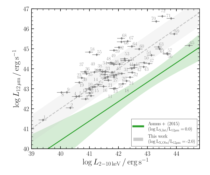
Figure 3: Predicted rest-frame $12\,\mu\rm m$ source luminosity (interpolated from the Mullaney11 infrared AGN spectral template) vs. the rest-frame observed $2-10\,\rm{keV}$ luminosity of our sample of Compton-thick AGN. The solid (green) line is the best fit correlation from Asmus15, together with the 1-$\sigma$ scatter in light green shading. All sources were assigned a 30% and 15% uncertainty to the X-ray and $12\,\mu\rm m$ luminosities, respectively. The sample shows diminished X-ray emission relative to $12\,\mu\rm m$ emission by a factor of greater than 2 orders of magnitude on average, indicative of Compton-thick obscuration. The average observed correlation is shown with a grey dotted line and shaded standard deviation. Labels refer to the ID column in Table LABEL:tab:sample.

3.2.1 Star Formation Contamination of $L_{\rm{12\,\mu m}}$

To test for infrared star formation contamination, we first used the $12\,\mu\rm m$ observations from Asmus14. This work minimised star-formation contamination in measuring mid-infrared fluxes of local sources by using high-angular resolution ($\lesssim 0\aas@@fstack{\prime\prime}4$) imaging with ground-based 8 m class telescopes. Such contamination would not be excluded from WISE-based measurements, that were used in our sample for these sources, due to the larger angular resolution (FWHM) of $6\aas@@fstack{\prime\prime}1$, $6\aas@@fstack{\prime\prime}4$, $6\aas@@fstack{\prime\prime}5$ and $12\aas@@fstack{\prime\prime}0$ for W1, W2, W3 and W4, respectively. 16 of our sample of 72 sources have measured fluxes in Asmus14. The average X-ray to mid-infrared flux ratio for these 16 sources was consistent with the equivalent ratio for the full sample. To fully account for this in the remainder of our sample without high angular resolution measurements, we conservatively use the average change in flux between WISE and Asmus14 (0.29 dex) added in quadrature to the original 15% uncertainty assigned to the template interpolated flux as the lower error bar for all sources lacking a mid-infrared observation from Asmus14, giving 0.30 dex. For the 16 sources with measured fluxes from Asmus14, we use the quoted rest-frame 12 $\mu$m luminosities and uncertainties therein.

3.3 Rest-frame Fe K$\rm{\alpha}$ line EWs

Due to the complexity associated with NGC 1068 (Bauer15), NGC 4945 (Puccetti14) and the Circinus Galaxy (Arevalo14), our simplified phenomenological model could not provide a reasonable description of the data for these sources. For this reason, we use the EWs quoted in Ricci15, converted to the rest-frame for the corresponding sources. Additionally, we did not have access to the spectral files for 4 high-redshift sources. The source of the EWs we use for our analysis are included in Table LABEL:tab:sample, column (12). In total, we computed the rest-frame neutral Fe K$\rm{\alpha}$ fluorescence line EW for 65/72 sources, as follows:

1. Any counts with $E\,<\,3\,\rm{keV}$ in the source rest-frame were ignored for Chandra (or $E\,<\,4\,\rm{keV}$ for NuSTAR) observations, in order to remove as much soft X-ray contamination from non-primary AGN sources as possible. Such sources include intrinsic AGN emission scattered into the line of sight, a relativistic jet, X-ray binaries present in the host or photoionised gas. Furthermore, all counts above 7 keV in the observed frame were excluded to account for the instrument-based sensitivities of Chandra. The corresponding upper limit for NuSTAR was $\sim$ 14–15 keV in the observed frame, optimising the measurement of the continuum over the most sensitive NuSTAR energy range.

2. In the low counts regime, we used Cash-statistics (Cash79, C-stat) during fitting. Spectra were either grouped to allow a minimum number of counts, or a minimum signal-to-noise (S/N) ratio per bin, while retaining enough spectral resolution for the Fe K$\alpha$ line. We generally favoured fitting with C-stat unless sources had enough counts or high enough S/N to warrant the use of $\chi^{2}$ statistics on a correspondingly S/N-binned spectrum. We experimented with different binning strategies within the sources fitted with C-stat, and found consistent outcomes.

3. Next we fitted each spectrum with a simplified phenomenological model consisting of photoelectric absorption acting on a composite power law plus a narrow Gaussian of $\mathrm{FWHM}\approx\,2\,$eV ($\sigma\,=\,1\,\mathrm{eV}$), modelling the observed continuum plus the narrow core of the Fe K$\rm{\alpha}$ fluorescence line. This model was used only to constrain the shape of the observed spectrum, and the EW of the Fe K$\alpha$ line. If a given source had an observed excess of emission in the softer energy band ($E\lesssim 4\,\mathrm{keV}$) an apec component was additionally included in the model to account for this. In xspec, this baseline model takes the form:

   model = gal_phabs $$\times$$ (apec +

   zphabs $$\times \Gamma$$ (zpowerlaw[ = 1.4] +

   zgauss[E_L = 6.4 keV])) (1)

   gal_phabs refers to an additional minor contribution to the absorption from the Galaxy. Items in square brackets refer to fixed parameters. Although many studies suggest the intrinsic power law of AGN have average photon indices of $\sim$ 1.9, we fit the spectra with a flatter (lower) photon index of 1.4, as this is closer to the value found for the flat ($<10$ keV) reflection spectra typically observed for Compton-thick AGN, and we required our model to provide a reasonable fit to the observed spectrum.

4. We then computed two-dimensional confidence contours over the zpowerlaw and zgaussian model component normalisations (whilst leaving $N_{\rm H}$ and, if required to describe the soft region of the observed spectrum, the apec normalisation, free).

5. These contours were translated to confidence on the Fe K$\rm{\alpha}$ EW, and plotted as a function of the statistical test difference from the best fit acquired (chi-squared or Cash-statistics depending on the source). This enables us to determine the minimum, and hence presumed best fit rest-frame EW, together with the 1-$\sigma$ uncertainty. Irrespective of using chi-squared or Cash-statistic, we use a delta statistic of +2.30 to represent the 1-$\sigma$ (68%) confidence level for two interesting parameters.

6. For sources in which the normalisation of the Fe K$\alpha$ line could not be constrained in the fit, we use the limit derived by xspec on this parameter to calculate an upper bound on the EW. For any sources that yielded an unphysical EW $>\,$5 keV, we set the limit to this value. This is applicable to 3 sources: CDFS 443, CDFS 454 & COSMOS 2180, with EW $\lesssim$ 12 keV, EW $\lesssim 48$ keV and EW $\lesssim 11$ keV, respectively. We defer the reader to the Appendix for the grouped spectrum used for each source.

3.4 Fitting procedure

Our final sample consists of 72 sources, including 18 upper limits on the EW. All sources without quoted luminosities in Asmus14 were assigned the same lower uncertainty of 0.3 dex on $12\,\rm{\mu}\rm m$ luminosity specified in Section 3.2. We then fitted a linear regression to the EW vs. rest-frame $12\,\rm{\mu}\rm m$ luminosity. To account for all the uncertainties present in our sample whilst determining a fit, our fitting procedure was as follows:

1. The dataset was bootstrapped by randomly sampling data points from the original whilst allowing repeats. The new dataset was the same size as the parent sample.

2. Each point in the bootstrapped dataset was randomly resampled depending on the uncertainty of each point, as follows:

   1. Non-detections/upper limits: new points were randomly drawn from a uniform distribution in the interval $[\rm{log}\,100\,\rm{eV},\rm{log\,limit\,[eV]}]$,

   2. Detections: A new value was generated from a Gaussian distribution with standard deviation given by the 1-$\sigma$ error being considered for that point.

   To avoid strongly unphysical values from biasing the simulations, we truncated the randomised EWs to between 100 eV and 5 keV.

3. A linear least-squares regression was carried out on the Monte Carlo simulated dataset using the scipy.linregress Python package. The Spearman’s Rank Correlation Coefficient ($\rho$) was then found using the scipy.spearmanr package for each fit.

4. Steps (i) – (iii) were repeated in order to obtain a distribution of gradients, y-intercepts and $\rho$ values for the original dataset.

4 RESULTS

Table LABEL:tab:sample includes details of each source used in our final sample, and the Appendix contains the best fit spectrum and EW contour for each source used, as well as the sources ruled out in our analysis. After carrying out 20,000 iterations, we obtain a best fit linear regression to the data of:

$$\rm{log}(\rm{EW_{\rm{Fe\,K\alpha}}/keV})=$$

$$\hskip 40.0pt-(0.08\pm 0.04)\,\rm{log}(L_{12\,\rm{\mu}\rm m}/10^{44}\,\rm{erg\,s}^{-1})+2.87\pm 0.05$$ (2)

Figure 4 shows all rest-frame $12\,\mu\rm m$ luminosities vs. rest-frame neutral Fe K$\rm{\alpha}$ fluorescence line EWs. Blue arrows represent upper limits. As a comparison to previous studies into the Iwasawa-Taniguchi effect, we further include the gradients of previous works: Iwasawa93, Page04, Bianchi07 and Ricci14, normalised to the same y-intercept at $10^{44}\,\rm{erg\,s}^{-1}$. We make this normalisation since the EWs we report for our sample are measured relative to the observed spectrum, which for Compton-thick obscuration is drastically different to the observed spectrum for unobscured AGN, not to mention our proxy for the bolometric luminosity is different to that previously used by other studies.

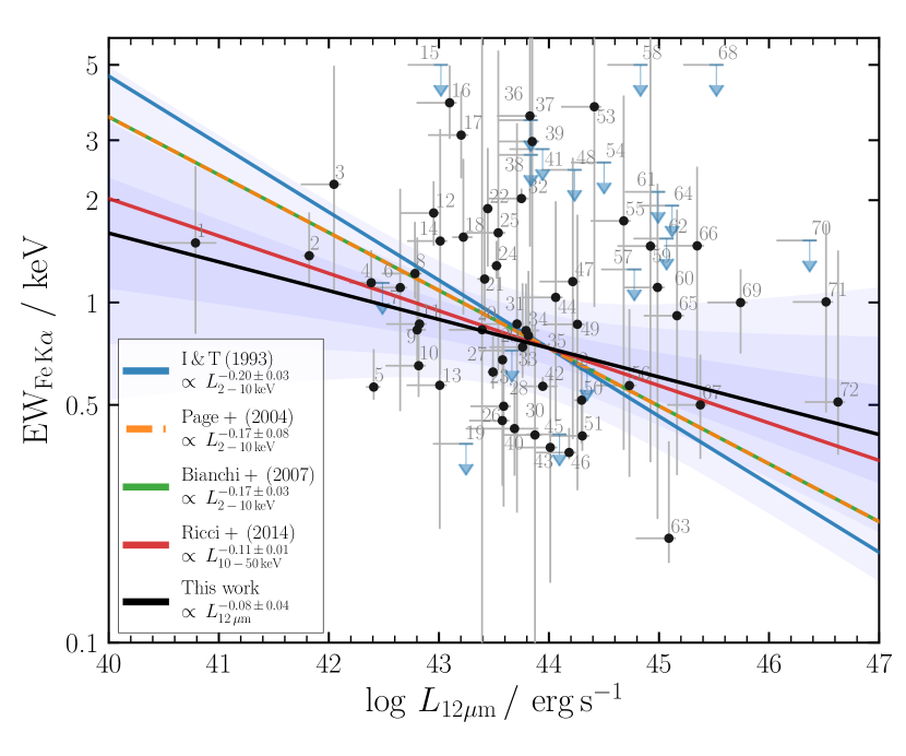
Figure 4: Plot of $L_{12\,\mu\rm m}$ vs. (rest-frame) neutral Fe K$\rm{\alpha}$ fluorescence line EWs. Blue arrows represent upper limits. As a comparison to previous studies into the Iwasawa-Taniguchi effect, we further include the gradients of previous works Iwasawa93, Page04, Bianchi07 and Ricci14. These correlations have all been renormalised to match our best fit y-intercept at $10^{44}\,\rm{erg\,s}^{-1}$ for comparison, since we are using the $12\,\mu\rm m$ luminosity, which is different from the intrinsic luminosity proxies used by other Iwasawa-Taniguchi effect studies. The blue shaded region represents the standard deviation from the mean of our best fit, with lighter shading corresponding to incrementally lower numbers of standard deviation.

To test the significance of the fit, we computed the Spearman’s Rank Correlation Coefficient ($\rho$) of the correlation for our sample, excluding upper limits. Upper limits were excluded since $\rho$ tests the strength of a monotonic relationship between variables, which can be dramatically effected by the large range of values/orders of variables attainable with the inclusion of limits in our Monte-Carlo based fitting method. This left 54 sources, and gave a value of $\rho\,=\,-0.28\pm 0.12$. Figure 5 shows the corresponding distribution in $\rho$ found, indicating a negative correlation to 98.7% confidence.

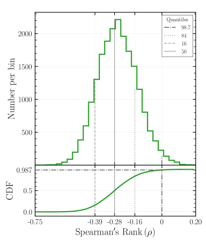
Figure 5: Distribution of Spearman’s Rank Correlation Coefficients ($\rho$) generated from 20,000 iterations of steps (1) - (3) of our fitting procedure, outlined in Section 3.4, for a dataset excluding all upper limits (54 in total). The 16th, 50th and 84th quantiles are shown with dashed, solid and dotted lines, respectively. The dotted (purple) line additionally shows the correlation to be negative to 98.7% confidence.

Our best fit gradient is fully consistent with Ricci14 within 1-$\sigma$ errors, who attempted to take into account time-averaging of the spectra for determining EWs - see Section LABEL:sec:discussion for further discussion on this result. The gradient found here is also flatter than the Bianchi07 best fit gradient, but consistent within 90% confidence. We include the distributions of our best linear fit gradients and y-intercepts in Figures LABEL:fig:m and LABEL:fig:c, respectively for the 20,000 iterations (including upper limits).