AGN contamination of galaxy-cluster thermal X-ray emission: predictions for eRosita from cosmological simulations

Abstract

In this study, we present a modelling of the X-ray emission from the simulated SMBHs within the cosmological hydrodynamical Magneticum Pathfinder Simulation, in order to study the statistical properties of the resulting X-ray Active Galactic Nuclei (AGN) population and their expected contribution to the X-ray flux from galaxy clusters. The simulations reproduce the evolution of the observed unabsorbed AGN bolometric luminosity functions (LFs) up to redshift $z\sim 2$, consistently with previous works. Furthermore, we study the evolution of the LFs in the soft (SXR) and hard (HXR) X-ray bands by means of synthetic X-ray data generated with the PHOX simulator, that includes an observationally-motivated modelling of an instrinsic absorption component, mimicking the torus around the AGN. The reconstructed SXR and HXR AGN LFs present a remarkable agreement with observational data up to $z\sim 2$ when an additional obscuration fraction for Compton-thick AGN is assumed, although a discrepancy still exists for the SXR LF at $z=2.3$. With this approach, we also generate full eROSITA mock observations to predict the level of contamination due to AGN of the intra-cluster medium (ICM) X-ray emission, which can affect cluster detection especially at high redshifts. We find that, at $z\sim 1\mbox{--}1.5$, for $20\mbox{--}40\%$ of the clusters with $M_{500}>3\times 10^{13}\,h^{-1}\rm{\,M_{\odot}}$, the AGN counts in the observed SXR band exceed by more than a factor of 2 the counts from the whole ICM.

1 Introduction

The presence of supermassive black holes (SMBHs) is nowadays known to be very common at the centre of massive galaxies and show properties, such as total mass, that appear to be correlated to the properties of their hosts, such as bulge stellar mass or velocity dispersion (e.g. Magorrian et al., 1998; Ferrarese & Merritt, 2000; Gebhardt et al., 2000; Tremaine et al., 2002; Ferrarese & Ford, 2005; Kormendy & Ho, 2013; McConnell & Ma, 2013). The nuclear activity due to matter accretion onto the central SMBH, however, is observed in only 1–10% of the galaxies, indicating that the co-evolution between active galactic nuclei (AGN) and host galaxy is a very complex and intermittent process.

In the case of brightest cluster galaxies (BCGs) in galaxy clusters, the importance of AGN activity is even more crucial, as it affects not only the star formation activity within the BCG Benson et al. (2003); Croton et al. (2006) but also the wider environment around it and the hot gas filling the cluster potential well, i.e. the intra-cluster medium (ICM) Fabian et al. (2003); McNamara et al. (2000, 2005); Voit & Donahue (2005). ICM thermal and chemical properties in the cores of clusters show the effects of the central AGN, depending on its growth and evolution (e.g. Gitti et al., 2012, and references therein). In fact, if no efficient feedback mechanism was in place at the centre of galaxy clusters, massive cooling flows were to be expected as a consequence of the radiative cooling of the ICM (see Fabian et al., 1984; Sarazin, 1986; Fabian, 1994), whose temperatures reach $10^{7}$–$10^{8}$ K emitting in the X-rays with typical luminosities of $10^{43\mbox{--}45}\rm{\,erg/s}$. As an observable signature of this process, we should expect large reservoirs of cool gas in the centre of clusters, especially in those with a high-density core and centrally peaked X-ray surface brightness (cool-core clusters), resulting in considerable star formation rates in the BCG. This so-called “cooling flow” scenario Fabian (1994) is however not observed and a heating mechanism able to prevent such gas radiative cooling and star formation in the core must be in place (Peterson et al., 2001; David et al., 2001; Peterson & Fabian, 2006, and references therein). It is commonly accepted that this role is played by AGN feedback (see review articles by Gitti et al. 2012 and Fabian 2012, and references therein).

Statistically, studies of the populations of AGN at different redshifts, for instance through the construction of luminosity functions (LFs) at various wavelenghts, are particularly useful to investigate the growth history of SMBHs in the Universe and to infer constraints on their co-evolution with the host galaxy and the environment. Several observational campaigns have been dedicated to this scope (e.g. Maccacaro et al., 1983, 1984; Maccacaro et al., 1991; Boyle et al., 1993, 1994; Page et al., 1996; Boyle et al., 2000; Wolf et al., 2003; Ueda et al., 2003; Simpson, 2005; Barger & Cowie, 2005; La Franca et al., 2005; Richards & et al., 2006; Bongiorno & et al., 2007; Silverman et al., 2008; Hasinger, 2008; Croom et al., 2009; Aird et al., 2010, 2015; Assef et al., 2011; Fiore et al., 2012; Merloni & et al., 2014; Buchner et al., 2015; Fotopoulou et al., 2016; Ranalli & et al., 2016).

Given the complexity of the phenomena, however, it is very difficult to capture the details of the cycle regulating the gas inflow towards the cluster centre, the accretion of this gas onto the central SMBHs, the triggering of powerful AGN activity and the consequent release of energy from the AGN into the surrounding medium, that prevents further gas accretion and quenches star formation.

The challenge to include the modelling of these phenomena within simulations is mainly related to the involved time-scales, which differ largely — e.g. the time-step of the simulation compared to the time-scale over which the process of gas accretion onto the BH (and therefore the following variation of the AGN luminosity) occurs. The estimation of AGN luminosities from cosmological simulations that include SMBHs, and account for the modelling of gas accretion onto them, should therefore be regarded mainly from a statistical perspective. The possibility to correctly model a realistic population of AGN that originates directly from the SMBH population within a cosmological context is nevertheless the key step to study and understand the SMBH evolution and their impact on physical properties of galaxies and clusters.

Several theoretical works, both numerical and semi-analytical, have also focused on the population of SMBHs and their relation to the small-scale galactic environment, and on the constructions of luminosity and mass functions that are crucial to be compared against observational evidences in order to interpret them as well as to validate the modelling itself. In particular, cosmological hydrodynamical simulations have been performed in the past two decades with the specific purpose of studying the statistical properties of the simulated SMBHs and AGN populations, such as LFs, within a cosmological context (e.g. Di Matteo et al., 2008, 2012; McCarthy et al., 2010; McCarthy et al., 2011; Booth & Schaye, 2011; Degraf et al., 2010, 2011; Haas et al., 2013; Hirschmann et al., 2014; Sijacki et al., 2015; Steinborn et al., 2015, 2016; Koulouridis et al., 2017), including various different implementations of the AGN feedback model (e.g. Di Matteo et al., 2005; Springel et al., 2005; Hopkins et al., 2006; Sijacki et al., 2007; Booth & Schaye, 2009; Fabjan et al., 2010; Barai et al., 2014; Steinborn et al., 2015).

Cosmological hydrodynamical simulations of galaxy clusters have also shown how the presence of AGN feedback, in addition to stellar one, can impact on the entropy, metallicity and thermal properties in cluster cores, by reducing the amount of high density and low temperature gas in the centre which causes excessive star formation. This eventually contributes to a diversity of thermal and chemical properties of the cores that resemble the observed ones (e.g. Hahn et al., 2015; Rasia et al., 2015; Martizzi et al., 2016; Planelles et al., 2017; Biffi et al., 2017; Vogelsberger et al., 2017).

The comparison between numerical results and observational data is crucial in order to assess the reliability of the models included in the simulations and to interpret the observational results themselves, although comparison studies of this kind have been relatively limited so far. For a more direct and faithful comparison, synthetic data can be derived from the simulations. In a recent work, Koulouridis et al. (2017) derived mock X-ray AGN catalogs from the cosmo-OWLS simulation suite, in order to investigate the demographics of the AGN population in the simulations. They find that the unabsorbed X-ray luminosity function accurately reproduces the observed one over 3 orders of magnitude in X-ray luminosity from $z=0$ out to $z=3$, as well as the Eddington ratio distribution and the projected clustering of X-ray AGN.

For a realistic population of simulated BHs and AGN, in terms of comparison to observational evidences, simulations and mock X-ray data are powerful tools to constrain the possible contribution from AGN X-ray emission to the ICM emission of the host cluster. In fact, X-ray observations point out the difficulty in detecting an active AGN during its outburst phase within the BCG of a galaxy cluster. This is essentially due to the ambiguity of disentangling the AGN point source emission from the X-ray peak associated to the cluster core, especially in centrally-peaked CC clusters and at high redshift for X-ray telescopes with moderate (more than a few arcseconds) spatial resolution. In fact, this will be crucial for future X-ray survey instruments like eROSITA, for which the PSF in scanning mode will be large (Half-Energy Width $\sim 26\mbox{--}28"$ and positional accuracy of point sources $\sim 7\mbox{--}15"$) and will make it very difficult to resolve the central core in CC clusters. In such cases, cluster detection can be challenging, especially at high redshift, since the instrument spatial resolution will not allow to distinguish the extended diffuse emission of the ICM and, in case of powerful AGN in cluster BCGs, the X-ray emission will be likely associated to them rather than to the hosting cluster. Nevertheless, if the host galaxy of the detected AGN is a member of a massive cluster, then the X-ray emission from the AGN can be a minor fraction of the total AGN and ICM emission. The situation where the point source is classified as an AGN and the cluster remains uncatalogued contributes to the rarity of selecting active AGN at the centre of massive clusters and constitutes an important selection bias that should be taken into account especially in future surveys. A way to overcome this problem, by combining X-ray and optical data, is presented in a recent work by Green et al. (2017), where they look for evidences of the presence of a rich cluster around ROSAT X-ray sources identified as AGN, by searching for overdensities in red-sequence galaxies.

In such a framework, we aim at investigating the population of SMBHs in the Magneticum Pathfinder Simulation (see Section 2) in terms of X-ray LFs and their evolution with redshift, in comparison to observational findings. Given a realistic AGN population, we ultimately intend to use simulations to predict the importance of AGN contamination to the X-ray luminosity and observed emission from galaxy clusters. To this scope, we set up a model for the AGN X-ray emission that accounts for both intrinsic absorption and luminosity- and redshift-dependent obscuration fractions, and finally construct synthetic observations of the simulated clusters with AGN. We consider the instrumental specifications of the up-coming X-ray satellite eROSITA in order to predict the relative contribution from AGN and ICM to the observed X-ray fluxes, which will affect the detection of galaxy clusters out to redshifts 1–1.5.

More specifically, the paper is organized as follows. In Section 3 we first discuss the theoretical modelling of the AGN bolometric emission, from which we reconstruct the bolometric LFs, and then apply observationally-motivated bolometric corrections to derive the AGN intrinsic luminosities in the soft ([$0.5$–$2$] keV) and hard ([$2$–$10$] keV) X-ray band (hereafter: SXR and HXR, respectively). As a step further, we apply an X-ray photon simulator to the simulations to simultaneously mimic the X-ray emission from both cluster ICM and AGN sources, following the approach outlined in Section 4. In Sections 5 and 6 we present our main results on the reconstructed SXR and HXR AGN LFs, with and without intrinsic absorption, and on the relative contribution of AGN in clusters with respect to the X-ray emission from the diffuse ICM, as expected in particular from eROSITA observations. Finally, we draw our conclusions in Section 7.

2 Cosmological hydrodynamical simulations

In this work we use one of the simulations that are part of the Magneticum Pathfinder Simulation. In particular, the simulation used comprises a comoving volume of $352\,h^{-1}\rm{\,Mpc}$ and a mass resolution of $m_{\rm DM}=6.9\times 10^{8}\,h^{-1}\rm{\,M_{\odot}}$, for the dark matter (DM) component, and $m_{\rm g}=1.4\times 10^{8}\,h^{-1}\rm{\,M_{\odot}}$, for the gas. We refer to this run as Box2/hr (see also Hirschmann et al., 2014), where hr denotes the high resolution of the run (initially resolved with $2\times 1564^{3}$ particles). The cosmology adopted refers to the 7-year WMAP results, that is we assume $h_{0}=0.704$, for the scaled Hubble parameter, and $\Omega_{\rm 0M}=0.272$ and $\Omega_{\rm 0\Lambda}=0.728$, for the matter and Cosmological constant density parameters. Also, we set the initial power-spectrum index to $n=0.963$ and normalize it to $\sigma_{8}=0.809$.

2.1 The numerical code

These simulations have been performed with the parallel TreePM-SPH code Gadget-3, an extended version of the Gadget-2 code presented in Springel (2005). This includes an entropy-conserving formulation of the SPH Springel & Hernquist (2002), a higher order kernel based on the sixth-order Wendland kernel Dehnen & Aly (2012) with 295 neighbors, a low-viscosity scheme and a treatment for artificial diffusion that allow for a better treatment of turbulence and gas mixing Dolag et al. (2005); Beck et al. (2016). The code also accounts for the treatment of a wide range of physical processes governing the evolution of the baryonic component. In fact, it accounts for metal-dependent radiative cooling (following Wiersma et al., 2009), for the presence of the cosmic microwave background (CMB) and of a UV/X-ray uniform ionizing background radiation from quasars and galaxies, as computed by Haardt & Madau (2001). Star formation and feedback from galactic winds driven by supernovae (SN) explosions (with a velocity of $350\rm{\,km/s}$) are implemented following the original formulaiton by Springel & Hernquist (2003), and a description for black hole (BH) growth and feedback from active galactic nuclei (AGN) is also incorporated Fabjan et al. (2010). The code comprises as well a detailed model for chemical enrichment, where the production of heavy elements is implemented according to proper stellar population life-times and yields, for supernovae type Ia (SNIa) and type II (SNII), and for intermediate- and low-mass stars in the asymptotic giant branch (AGB) phase (see Tornatore et al., 2003, 2007). The metal cooling and enrichment is followed by tracking directly 11 metal species (H, He, C, N, O, Ne, Mg, Si, S, Ca, Fe). Additionally, we include isotropic (physical) thermal conduction (with $1/20$ of the classical Spitzer value) Dolag et al. (2004) and passive magnetic fields Dolag & Stasyszyn (2009).

3 Modelling the AGN X-ray emission

In this section we describe the theoretical estimation of AGN bolometric, SXR and HXR luminosities from the simulations, and present results on the bolometric AGN LFs.

3.1 Theoretical estimation of the AGN luminosity

The bolometric luminosity associated to any AGN source in the simulation can be calculated starting from the principal BH properties traced directly by the simulation itself, such as its mass and (large-scale) accretion rate, and by assuming some efficiency value ($\varepsilon_{r}$).

In the standard scheme used to estimate the (bolometric) radiated luminosity from accretion onto a BH, we have:

$$\rm{\,L_{\rm rad}}=\varepsilon_{r}\dot{M}c^{2},$$ (1)

where typically $\varepsilon_{r}=0.1$ (see e.g. Maio et al., 2013, and references therein).

Alternatively, one can choose a more detailed modelling that takes into account the specific accretion phase which the AGN source is undergoing, determined according to its BH accretion rate (BHAR). Namely, the BHAR

$${\rm BHAR}=\frac{\dot{M}}{\dot{M}_{\rm Edd}}$$ (2)

is used to distinguish different radiation regimes, following Fig. 1 of Churazov et al. (2005). Specifically, the radiative power (i.e. AGN luminosity) is calculated differently for radiatively efficient and inefficient AGN:

$$\frac{\rm{\,L_{\rm rad}}}{L_{\rm Edd}}=\left\{\begin{aligned} &\varepsilon_{r}\left(\!10\frac{\dot{M}}{\dot{M}_{\rm Edd}}\!\right),&\quad&{\rm if~{}BHAR}>0.1\\ &\varepsilon_{r}\left(\!10\frac{\dot{M}}{\dot{M}_{\rm Edd}}\!\right)^{2},&&{\rm if~{}BHAR}<0.1\,\end{aligned}\right.$$ (3a)

corresponding to the radiatively efficient (quasar) ($${\rm BHAR}>0.1 {\rm BHAR}<0.1$$) and inefficient () regime, respectively. We recall that the Eddington quantities read:

$$L_{\rm Edd}=\frac{4\pi Gm_{p}c}{\sigma_{t}}M_{\rm BH}$$ (3b)

and

$$\dot{M}_{\rm Edd}=\frac{L_{\rm Edd}}{\varepsilon_{r}c^{2}}=\frac{4\pi Gm_{p}}{\varepsilon_{r}\sigma_{t}c}M_{\rm BH}\,.$$ (3c)

Provided the values of $$M_{\rm BH} \dot{M} \varepsilon_{r} \varepsilon_{r}=0.1$$ and from the simulation, we only need to assume a value for the efficiency . Also in this second approach, we use .

For any BH particle in the simulation, we can therefore compute its (bolometric) luminosity $\rm{\,L_{\rm bol}}$ and derive luminosity functions (LFs), in order to explore the properties of the AGN population. Here and in the following, we refer to the bolometric luminosity $\rm{\,L_{\rm bol}}$ as the theoretical estimation of the AGN luminosity, calculated either adopting the standard estimation or the BHAR-dependent scheme.

The AGN LFs obtained from our simulation are shown in Fig. 1, for different redshifts between $\sim 0.1$ and $\sim 2$. The three curves reported in the Figure are calculated for the AGN sources in our simulations considering the standard bolometric luminosity estimate Eq. (1) (“std”) or the scheme by Churazov et al. (2005). For the latter, we consider either the case expressed in Eq. (3a) (“CH05 (a)”) or the following modified version, where we adopt a transition value between radio and quasar mode of ${\rm BHAR}=0.05$ (see also Merloni & Heinz, 2008) (“CH05 (b)”):

$$\frac{\rm{\,L_{\rm rad}}}{L_{\rm Edd}}=\left\{\begin{aligned} &\varepsilon_{r}\left(\!10\frac{\dot{M}}{\dot{M}_{\rm Edd}}\!\right),&\quad&{\rm if~{}BHAR}>0.05\\ &\varepsilon_{r}\left(\!14.1\frac{\dot{M}}{\dot{M}_{\rm Edd}}\!\right)^{2},&&{\rm if~{}BHAR}<0.05\,,\end{aligned}\right.$$ (3d)

where we still assume $\varepsilon_{r}=0.1$. Being still a standard reference in the field, we compare the LFs from the Magneticum Pathfinder Simulation against observational data by Hopkins et al. (2007), in which bolometric luminosities are obtained by correcting observed luminosities in different energy bands.

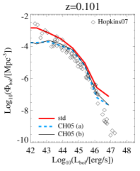
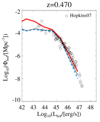
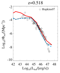
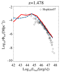
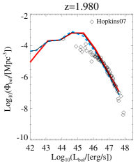
Figure 1: Bolometric AGN LFs computed for the Box2/hr at redshift $z\sim 0.1,0.47,0.52,1.04,1.48,1.98$ (from top-left to bottom-right). Different lines refer to different estimates of the AGN bolometric luminosity: the thick solid red line — “std” — corresponds to Eq. (1), the dashed blue line — “CH05 (a)” — to Eq. (3a) with a transition value for the ${\rm BHAR}$ of 0.1 and the thin solid black line — “CH05 (b)” — to Eq. (3d) with a transition value for the ${\rm BHAR}$ of 0.05. For comparison we also report observational data by Hopkins et al. (2007) (black diamonds).

From the panels in Fig. 1 we note that there is an overall reasonable match in the redshift range $0.47<z<2$, especially in the intermediate-high luminosity end. At redshift higher than $1$ we note a tendency to overestimate the observed number of lower-luminosity clusters. Similar results were also obtained in Hirschmann et al. (2014) for the same set of simulations, where the authors show that a discrepancy w.r.t. data rather appears at higher redshifts, $z\gtrsim 2$.

From the comparison in Fig. 1, we conclude that in the luminosity and redshift range where the simulation results are in reasonable agreement with the observational data, the “std” and both “CH05 (a),(b)” models do not differ significantly. At low redshift, $z\lesssim 1$, the low-luminosity end of the observed LFs is better reproduced by the “std” estimate.

Given these results, and for simplicity, we adopt in the following the standard estimation given by Eq. (1) (thick solid red curves).

3.2 Bolometric corrections: $\rm{\,L_{\rm SXR}}$ and $\rm{\,L_{\rm HXR}}$

The estimation of $\rm{\,L_{\rm bol}}$ is nevertheless not enough to constrain the AGN X-ray emission model nor to fully compare the properties of the simulated AGN population against observed datasets and LFs. Therefore, it is particularly useful to derive X-ray luminosities in specific energy bands, namely the SXR and HXR bands.

To this purpose, we convert the bolometric luminosities into SXR and HXR luminosities assuming the bolometric corrections proposed by Marconi et al. (2004), which can be approximated by the following third-degree polynomial fits

$$\log(\rm{\,L_{\rm HXR}}/\rm{\,L_{\rm bol}}) =-1.54\!-\!0.24\mathcal{L}\!-\!0.012\mathcal{L}^{2}\!+\!0.0015\mathcal{L}^{3}$$ (4)

$$\log(\rm{\,L_{\rm SXR}}/\rm{\,L_{\rm bol}}) =-1.65\!-\!0.22\mathcal{L}\!-\!0.012\mathcal{L}^{2}\!+\!0.0015\mathcal{L}^{3}$$ (5)

with $\mathcal{L}=\log(\rm{\,L_{\rm bol}}/L_{\odot})-12$, and derived for the luminosity range $8.5<\log(\rm{\,L_{\rm bol}}/L_{\odot})<13$ (see Fig. 3(b) in Marconi et al., 2004). The reason for this choice is that the corrections are derived from template spectra, rather than from the average observed AGN spectral energy distribution (SED), with the goal of obtaining an estimate of the intrinsic AGN luminosity. This, in principle, is closer to the theoretical estimates of $\rm{\,L_{\rm bol}}$ derived from simulations. In particular, the spectral model used by Marconi et al. (2004) consists, in the X-ray band beyond 1 keV, of a single power law, with a typical photon index of $\sim 1.9$ and an exponential cut-off at $\sim 500$ keV, plus a reflection component. The template spectra, as well as the obtained corrections, are redshift independent.

Here and in the following, the SXR and HXR bands are considered to be rest-frame energies, unless otherwise explicitly stated (i.e. for the mock results in Secs. 6.3.1–6.3.2).

4 Synthetic X-ray emission

In this section we describe the modelling of the synthetic X-ray ICM and AGN emission form the simulations, with special attention to the AGN intrinsic absorption.

4.1 PHOX X-Ray photon simulator

In the present work we make use of the PHOX code (Biffi et al., 2012; Biffi et al., 2013, for further details) in order to generate X-ray synthetic observations from the ICM and AGN sources in the simulation. The PHOX X-ray photon simulator consists of three separate modules:

• in unit 1 the ideal photon emission in the X-ray band is computed for every emitting source by assuming a model spectrum, which is sampled statistically with a discrete number of photons and stored in a data cube that matches the simulation cube itself;

• in unit 2 a projection is applied, photon energies are Doppler-shifted according to the line-of-sight motion of the original emitting source and a spatial selection can additionally be considered;

• lastly in unit 3 realistic observing time and detector area are considered, and the ideal photon list is eventually convolved with the specific instrumental response of a chosen X-ray telescope.

This code has been applied to simulations of galaxy clusters to study the X-ray properties of the hot diffuse ICM Biffi et al. (2012); Biffi et al. (2013); Biffi et al. (2014); Biffi & Valdarnini (2015); Cui et al. (2016), by modelling the X-ray emission (bremsstrahlung continuum and metal emission lines) of the hot gas in the simulated clusters.

Nevertheless, the very general approach adopted allows to treat as well different X-ray sources traced by the simulations, provided that the corresponding emission model is constrained from the simulation and included in unit 1. Given the modular design of PHOX, the projection and convolution phases (unit 2 and unit 3) can be then applied to the photon cube independently of the different nature of the emitting source.

In this study, we present and employ an extension of PHOX that generates the sythetic X-ray emission from AGN-like sources included in the simulations.

4.2 ICM X-ray emission

The modelling of the synthetic X-ray emission from the ICM in siulated clusters is done by computing the emitted X-ray spectrum for every hot-phase gas element in the simulations, depending on its intrinsic thermal and chemical properties (namely density, temperature, global metallicity or singular element abundances). In particular, we assume for every gas element a single-temperature VAPEC thermal emission model with emission lines due to heavy elements Smith et al. (2001), implemented in XSPEC Arnaud (1996).

For further details on the modelling of the ICM X-ray emission, we refer the interested reader to the descriptions provided in Biffi et al. (2012); Biffi et al. (2013).

4.3 AGN X-ray emission: spectrum parameters

The modelling of the AGN X-ray emission in the PHOX code follows a very similar approach to the one implemented for the ICM emission. Given the BH properties calculated in the simulation (as described in Sections 3.1 and 3.2), for each AGN source element we can constrain the particular shape of the emission model spectrum and generate the associated (ideal) list of emitted X-ray photons.

The main difference in treating BH sources, instead of gas elements, resides in the different X-ray emission model expected. Instead of modelling the emission like a thermal bremsstrahlung continuum with metal emission lines, such as for the ICM, we need to assume a different spectral model. X-ray observations show evidence that all AGN sources share an intrinsic power law spectrum of the form $E^{-\alpha}$, with a photon index $\alpha$ (e.g. Zdziarski et al., 2000) that varies in the range 1.4–2.8 with a Gaussian distribution peaked around $\sim 1.9$–$2$. Thus, we assume a single, redshifted power law:

$$A(E)=[K(1+z)][E(1+z)]^{-\alpha}\left(\frac{1}{1+z}\right),$$ (6)

where $K$ is the normalization, $\alpha$ is the photon index (spectrum slope) and $z$ is the redshift of the source. Integrating the spectrum in Eq. (6) between two observed energies, $E_{1}$ and $E_{2}$, one can obtain the observed flux (and then luminosity) of the source.

In order to calculate the fiducial model for every BH source (represented by particles in the Lagrangian-based simulations we use here) in the simulation output, it is required to estimate the spectrum normalization and slope parameters, $K$ and $\alpha$. For each BH, these can be directly constrained from its the global properties, as sketched in the following.

• For any BH particle, we compute $\rm{\,L_{\rm bol}}$ from the simulation data and convert it to (rest-frame) $\rm{\,L_{\rm SXR}}$ and $\rm{\,L_{\rm HXR}}$ through the bolometric corrections (4) and (5) (Secs. 3.1 and 3.2).

• We assume a spectrum for an AGN-like source as in Eq. (6), so that the luminosity for a given (observed) $(E^{1},E^{2})$ energy band is given by:

  $$L_{\left(E^{1},E^{2}\right)}=F\int_{E^{1}}^{E^{2}}[K(1+z)][E(1+z)]^{-\alpha}\!\left(\frac{1}{1+z}\right)\!E{\rm d}E,$$ (7)

  where F is the rescaling factor to convert the flux (resulting from the integration) into the luminosity.

• From Eq. (7), the luminosities in the (restframe) SXR and HXR energy bands are given by:

  $$\left\{\!\!\begin{aligned} \rm{\,L_{\rm SXR}}&=F\!\int_{0.5/(1+z)}^{2/(1+z)}[K(1+z)][E(1+z)]^{-\alpha}\!\left(\frac{1}{1+z}\right)\!E{\rm d}E\\ \rm{\,L_{\rm HXR}}&=F\!\int_{2/(1+z)}^{10/(1+z)}[K(1+z)][E(1+z)]^{-\alpha}\!\left(\frac{1}{1+z}\right)\!E{\rm d}E\end{aligned}\right.\!$$ (8)

  where $\rm{\,L_{\rm SXR}}$ and $\rm{\,L_{\rm HXR}}$ are the values estimated from the simulation. In order to mimic the observed scatter in these relations, we also add to both $\rm{\,L_{\rm SXR}}$ and $\rm{\,L_{\rm HXR}}$ a Gaussian scatter with $\sigma=0.1$, in logaritmic scale.

• Solving the system of equations (8), we can constrain the specific values for $K$ and $\alpha$.

In Fig. 2 we show the reconstructed distributions of slopes found by our approach from the AGN in the simulation box analysed with PHOX. In the figure, we show the distribution for 4 example simulation snapshots between $z\sim 0.10$ and $z\sim 2.3$. The result seems in broad agreement with the typical expectations from the observed distribution (which we consider centered on $\alpha=1.9$ — long-dashed orange line). We note nevertheless a mild shift of the distribution peak towards lower $\alpha$ values from $z\sim 2$ to $z\sim 0$. This is likely related to the redshift evolution of the LFs, which are used together with bolometric corrections to constrain the slope.

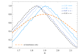
Figure 2: Distribution of the slopes computed for the emission spectra of the AGN in the simulations used in PHOX unit 1, for various redshifts between $0.1$ and $2.3$, as in the legend. For comparison, we also report the typical distribution expected from observations (orange dashed line).

By reconstructing the normalization and slope, $K$ and $\alpha$, for every BH we are able to compute the corresponding AGN spectrum by adopting the zpowerlw model embedded in the XSPEC package. This can be assumed to well represent the intrinsic power-law emission of the source in the energy range interesting for this work ($<50\,$keV).

4.3.1 Absorption

As suggested by many observational works, AGN sources also show evidences for the presence of obscuring material (i.e. the torus) in the vicinity of the central BH, which causes a partial absorption of the emitted radiation. Therefore, any modelling using a pure power law is too simplistic to mimic the observed properties of AGN and, even in the simplest case, it is required to account for an intrinsic absorption component.

Indeed, the bolometric AGN luminosities from our simulations have been compared in Section 3.1 to the observational results by Hopkins et al. (2007), in which the authors applied corrections to account for absorption and convert the observed luminosity into the intrinsic, bolometric one. Yet, in order to compare the SXR and HXR LFs of the AGN from the simulation to observed data, the correction for — or modelling of — obscuration is particularly important.

Several observational studies have focused on the characterization of the absorption depending on the source luminosity, and redshift (see, e.g., studies by Hasinger, 2008; Merloni & et al., 2014; Buchner et al., 2014, 2015; Fotopoulou et al., 2016; Ranalli & et al., 2016). The correction of instrinsic luminosities predicted by numerical studies by taking into account such observationally-motivated obscuration fractions has been for instance employed by Hirschmann et al. (2014), showing reasonable match between simulations and observations. Despite the large debate that still persists on the poorly constrained bolometric corrections and on the uncertainties on the fraction of obscured AGN, numerical studies have shown the importance of considering both in order to compare simulation-derived LFs and observational ones (see, e.g., recent works by Hirschmann et al., 2014; Sijacki et al., 2015; Koulouridis et al., 2017)

Here, however, we follow a different approach. Instead of correcting for absorption in the SXR and HXR LFs separately, following observed predictions, we rather assume an intrinsic absorption component for every AGN source in the simulation, with the aim of accounting for the effect of an obscuring torus present around the central BH.

In our implementation, the specific value of the obscurer column-density ($N_{H}$) is assigned to each AGN source in a probabilistic way, by assuming the estimated column-density distribution of the obscurer obtained in the study by Buchner et al. (2014) (see top-left panel of Fig. 10, in their paper) from a sample of 350 X-ray AGN in the 4 Ms Chandra Deep Field South. There, the authors analyse the AGN X-ray spectra and reconstruct the distribution of $N_{H}$ by using a detailed model for the obscurer, whose geometry is suggested to be compatible with a torus with a column density gradient, where the line-of-sight obscuration depends on the viewing angle and the observed additional reflection originates in denser regions of the torus.

Within the PHOX code, we include this in the construction procedure of the X-ray emission model from AGN-like sources. In particular, an intrinsic absorption component (at the redshift of the source) is added to the main power-law spectrum, together with the Galactic foreground absorption (which is the same for all the sources). For simplicity, we use a zwabs absorption component (at the redshift of the source) to represent the obscuring torus.

The complete model used to mimic the X-ray emission from AGN sources in the simulation (i.e. from BH particles) therefore is:

$${\tt wabs}\times{\tt zwabs}\times{\tt zpowerlw}\,,$$ (9)

where the first wabs represents the foreground Galactic-absorption component.

5 Reconstructed SXR and HXR LFs

In Fig. 3 we present the results of the modelling described in the previous subsections on the estimation of the SXR and HXR LFs and their comparison to observational data.

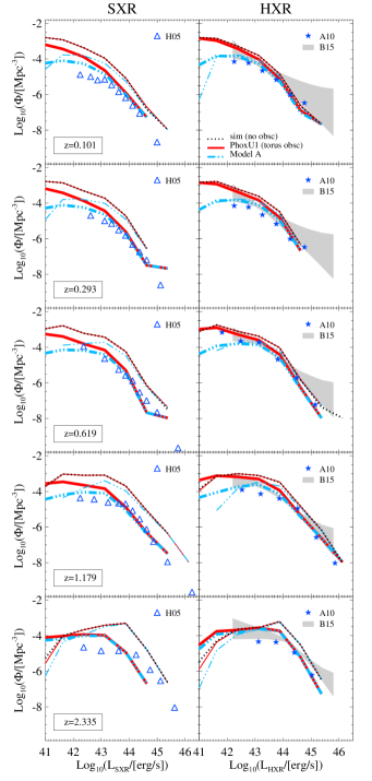
Figure 3: SXR (l.h.s. column) and HXR (r.h.s. column) AGN LFs built for the un-absorbed luminosities from the pure simulation prediction (dotted black line) and for the luminosities obtained from PHOX Unit 1 including the intrinsic torus absorption following Buchner et al. (2014) (solid red lines) and the (soft)luminosity- and redshift-dependent obscuration (in addition to intrinsic torus absorption) by Hasinger (2008) (Model A; dot-dot-dashed cyan lines). For the PHOX cases, we show both the LFs reconstructed from the un-absorbed intrinsic luminosities (thin lines) and from the absorbed ones (thick lines). For comparison, observed SXR and XHR LFs from Aird et al. (2010) (blue stars), Hasinger et al. (2005) (blue triangles) and Buchner et al. (2015) (grey shaded areas) are marked. From top to bottom, the panels refer to different redshifts $z\sim 0.1,0.3,0.6,1.2,2.3$.

In order to purely test the reliability of our treatment of AGN emission model and intrinsic obscuration, and to discuss it in comparison to observations, we do not construct at this stage complete mock observations for a given X-ray instrument. Simply, we consider the ideal photon list, generated from PHOX unit 1, for each AGN in the simulated cosmological volume. For the purpose of this test, we set the foreground Galactic absorption to zero, so that the ideal photons obtained from PHOX unit 1 can directly be used to calculate soft and hard X-ray LFs. Fiducial values for collecting area and observing time are significantly larger than realistic observational parameters, namely $A=2e3\,\rm{\,cm}^{2}$ and $\tau=50\rm{\,ks}$, respectively. This allows for luminosity estimates that closely resemble theoretical expectations. As assumed above, we construct the LFs for the rest-frame SXR and HXR energy bands, i.e. we integrate the flux from the observed photon lists within the redshifted energy bounds.

For different redshifts, from $z\sim 0.1$ up to $z\sim 2.3$, we compare in Fig. 3 the SXR and HXR LFs build from the simulation without any absorption (dotted black curves) and the ones reconstructed from PHOX.

For comparison, we overplot observational data presented by Aird et al. (2010), Hasinger et al. (2005) (blue stars and triangles, respectively), and Buchner et al. (2015) (grey shaded areas).

The LFs for the AGN processed with PHOX, taking into account the intrinsic torus absorption as in Sec. 4.3.1, are shown in Fig. 3 as red curves: the thick lines refer to the absorbed luminosities, whereas the thin lines indicate the LFs constructed from the intrinsic un-absorbed luminosities instead.

We show both LFs from un-absorbed and absorbed luminosities to show the two extreme cases, considering that different datasets make different assumptions on this point. In the SXR band especially, datasets that include only un-absorbed (type I) AGN, like those by Hasinger et al. (2005), directly employ the observed un-corrected luminosities and should be compared against simulated thick curves, that are produced from PHOX absorbed luminosities directly. The agreement in this case is relatively good, especially at intermediate-high redshifts and luminosities $\gtrsim 10^{43}$ erg/s. Other observational datasets that include instead both absorbed and unabsorbed AGN and construct LFs from absorption-corrected luminosities, as in the case of Buchner et al. (2015), should be rather compared to the simulated LFs (thin lines) built from intrinsic luminosities. The difference between the two curves in the HXR band is not striking and the simulated results show an overall good agreement with observations up to redshift $z\sim 1.2$ (depsite a mild overestimation of the LFs around $L_{\rm HXR}\sim 10^{44}$ erg/s).

Interestingly, this intrinsic-absorption modelling (“PHOXU1 (torus obsc)” in Fig. 3) naturally improves the comparison between simulations and observations, both in the soft and in the hard X-ray bands, at the same time. In fact, while the simulated LFs typically over-estimate the number of AGN at all luminosity scales, the curves obtained from PHOX, including the intrinsic absorption, tend to shift towards the range occupied by the observed data points. This evidence stresses the reliability of our implementation, as in fact by assuming an observational-based distribution of intrinsic absorption for the torus around each AGN source in the simulations (whose scales cannot be directly probed due to resolution limits), we can statistically better reproduce the observed LFs, not only in the HXR band from which the observed distribution is derived, but also in the SXR band. In the following analysis, for the purpose of generating synthetic observations of clusters including ICM and AGN emission, we will therefore use for the AGN component this model including an instrinsic torus-like absorption (“PHOXU1 (torus obsc)” in Fig. 3).

As previously mentioned, while some observational studies comprise both absorbed and unabsorbed AGN Buchner et al. (2014); Aird et al. (2015); Buchner et al. (2015), other datasets especially in the SXR band specifically refer to unabsorbed (type I) AGN, as for the LFs by Hasinger et al. (2005) reported in Fig. 3. In order to compare more faithfully simulation results to this kind of observations, we also generate LFs from AGN processed with PHOX by statistically excluding some of the sources according to an obscuration fraction that depends on the source SXR luminosity and redshift, as suggested by many observational evidences (e.g. Ueda et al., 2003; La Franca et al., 2005; Simpson, 2005; Hasinger et al., 2005; Hasinger, 2008; Ueda et al., 2014; Liu et al., 2017).

In particular, for this additional test and with the only purpose of comparing with data, we derive absorbed LFs from PHOX by adopting also the statistical obscuration fraction proposed by Hasinger (2008), where the fraction of obscured AGN ($f_{\rm obsc}$), at $z<2$, is given by:

$$f_{\rm obsc}(z,L_{\rm SXR})=-0.281\left(\log(L_{\rm SXR})-43.5\right)+0.279\,(1+z)^{\beta},$$ (10)

with $\beta=0.62$ providing the best fit to their bservational data. For higher redshifts, $z>2$, the value of $f_{\rm obsc}$ remains approximately the same as for $z=2$:

$$f_{\rm obsc}(z,L_{\rm SXR})=-0.281\left(\log(L_{\rm SXR})-43.5\right)+0.551.$$ (11)

In Fig. 3 we also report the LFs derived with this approach, marked as Model A (cyan, dot-dot-dashed lines). Essentially, we apply the relations (10) and (11) to the intrinsic $\rm{\,L_{\rm SXR}}$, as predicted by the simulations, in order to stochastically decide whether the AGN will be obscured or not, depending on its luminosity and redshift.

Given that studies like those by Hasinger et al. (2005) or Aird et al. (2010) do not explicitly correct the luminosities by the absorption, even though they still include some moderatly obscured AGN (with intrinsic column densities $N_{H}<10^{23}$ cm^-2), after considering the statistical obscuration fraction only the “observable” AGN are processed with PHOX, and to those, despite not being optically-thick, we still assign a torus absorption value (from the $N_{H}$ distribution by Buchner et al. (2014)) to account for partial obscuration. We note that this is an extreme limit that might overestimate the effect of obscuration.

With respect to the LFs derived from PHOX including the torus absorption without any explicit luminosity and redshift dependency, the Model A produces a decrease, at all redshift, in the LFs at the low-luminosity end ($\rm{\,L_{\rm SXR}}\lesssim 10^{43}$ erg/s and $\rm{\,L_{\rm HXR}}\lesssim 10^{44}$ erg/s), where absorption effects are more severe, whereas no significant change is observed in the high-luminosity tail. In general, this additional modelling of the luminosity- and redshift-dependent obscuration, combined with the intrinsic absorption implemented within PHOX, contributes to further improve the comparison against the observed luminosity functions by Hasinger et al. (2005) and Aird et al. (2010), reported in Fig. 3. The improved agreement with observed LFs is particularly evident in the low redshift bins. Even for Model A we show both LFs for absorbed and intrinsic luminosities (thick and thin lines, respectively), to emphasize the two extremes. Like before, the most significant differences are visible in the SXR band, while no strong effects are found in the HXR. In particular, we note that the comparison against the observations by Hasinger et al. (2005) is more faithful when absorbed luminosities are employed (thick cyan curves), and in this case the agreement is also overall better.

In general, there are large uncertainties and differences characterising different observational datasets, e.g. about the definition of obscured or un-obscured AGN depending on the value of $N_{H}$ or on the use of absorption-corrected or observed luminosities to build up the LFs. For this reason, in our implementation within PHOX, we assign a torus obscuration component to each observed AGN (according to the Buchner et al. (2014) distribution) but do not include any specific luminosity or redshift dependency of the obscuration fraction.

6 ICM and AGN X-ray emission in simulated clusters

In this section we present the simulation results on the X-ray emission from AGN in galaxy clusters, and its contribution to the global X-ray emission from the ICM.

6.1 Simulated data set

We extract a sample of cluster-size haloes, at various cosmic times, from the Box2/hr cosmological volume of the Magneticum Pathfinder Simulation set. Specifically, we select all the haloes with $M_{500}>3\times 10^{13}\,h^{-1}\rm{\,M_{\odot}}$, at 9 redshift snapshots between $z\sim 0.07$ and $z\sim 2$, obtaining therefore catalogs which are complete both in mass and volume. At $z=0.07$ our sample comprises 1649 clusters with masses $3\times 10^{13}\lesssim M_{500}/[\,h^{-1}\rm{\,M_{\odot}}]\lesssim 1\times 10^{15}$, whereas at $z=1.98$ the sample includes 34 systems with $M_{500}$ spanning the mass range $3\mbox{--}6.5\times 10^{13}$.

6.2 Mock X-ray observations

In order to predict the relative importance of AGN emission with respect to the ICM X-ray luminosity, we generate synthetic eROSITA observations out of the clusters in the simulation. Specifically, we apply PHOX to the catalogs of simulated clusters, considering both the ICM and the AGN components in the clusters. Ideal photon lists have been then generated for (i) the ICM X-ray emission (as outlined in Sec. 4.2) and (ii) the combined emission from ICM and AGN within the clusters (as outlined in Sections 4.3 and 4.3.1). For the AGN emission, we only include the modelling of the intrinsic torus absorption according to the absorber column-density distribution by Buchner et al. (2014), as in Eq. (9) (i.e. we model both Compton-thick and unabsorbed AGNs — but do not include any explicit luminosity- and redshift-dependent obscuration fraction). By means of the SIXTE dedicated simulator, we subsequently convolved the PHOX ideal photon lists with eROSITA instrumental specifications, in order to obtain observational-like data files. The ICM-only and AGN+ICM eROSITA-like images obtained with SIXTE are shown in Appendix A for two example clusters in our simulations. Since we do not include instrumental background, the received count rate effectively does not depend on the exposure time assumed (here we use 10 ks). eROSITA images and relative spectra have been extracted from the region enclosed within the projected $R_{500}$ for every cluster in the catalogs, at various redshift. This set up would correspond to simulating eROSITA pointed observations.

In this procedure, we assume for both source types a WABS model in XSPEC to include an artificial foreground Galactic absorption, with the value of the column density fixed to $N_{H}=10^{20}$ cm^-2.

6.3 AGN-to-ICM X-ray luminosity

Before inspecting the synthetic X-ray data, we investigate directly the simulations to predict the relation between the X-ray luminosity of the ICM and of the central AGN.

In Fig. 4, we show simulation results for the AGN-to-ICM luminosity ratio in the $[0.5$–$10]$ keV band, at various redshifts between $z\sim 0.1$ and $z\sim 2$. In particular, we consider the global ICM luminosity coming from the region within the virial radius and compare it to the intrinsic luminosity expected from the central AGN. To this scope we consider all AGN sources residing within the centremost region, i.e. $<5\%$ of the cluster virial radius, so that the $L_{\rm AGN}(<0.05R_{\rm vir})$ is in fact the total sum of their luminosities. We note, nonetheless, that for the majority of our clusters only the central AGN is comprised in that very central region. In order to estimate the intrinsic contribution predicted by the simulations, here luminosities are the theoretical values computed directly from the simulations (as in Section 3.2), so no absorption is included in the AGN emission. The effects of absorption and of the observational approach will be investigated through the mock analysis in Section 6.3.1.

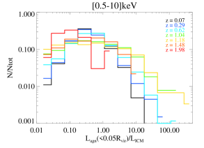
Figure 4: Differential distribution function of the AGN-to-ICM luminosities for all the central AGN sources of the selected clusters, at different redshifts between $z=0.07$ and $z\sim 2$. The AGN luminosity is the sum of the intrinsic luminosities (computed as in Section 3.2, without considering any absorption) of all AGN sources residing within $0.05\,R_{\rm vir}$, whereas the ICM luminosity is computed from the gas enclosed within the virial radius. Both luminosities are theoretical estimates calculated directly from the simulations in the [$0.5$–$10$] keV band.

We see from Fig. 4 that the distribution of the ratio

$$f_{L}\equiv L_{\rm AGN}(<0.05R_{\rm vir})/L_{\rm ICM}(<R_{\rm vir})$$ (12)

is typically centered on values comprised between $0.1$ and $1$. Up to $z\sim 0.6$ the median of the distribution slightly increases and then oscillates around similar values up to $z\sim 1$. The mean value, instead, increases from $z=0.07$ up to $z\sim 1.2$ and presents values even larger than 1 at redshift $0.6\lesssim z\lesssim 1.2$. At redshifts $z\gtrsim 0.6$ the distribution becomes broader and presents a prominent tail at values of $f_{L}$ much larger than 2. The broader shape of the distribution is still visible at $z\sim 1.5$, although the tail is truncated at $f_{L}\sim 10$. Instead, at $z\sim 2$, $f_{L}$ is again typically always lower than $\sim 1$. At that redshift, however, the cluster sample is much smaller and the AGN LFs indicate a poorer agreement between simulated and observational results. We cannot therefore derive strong constraints from these results at $z\sim 2$.

These findings indicate that considering the centremost AGN source(s) only, their intrinsic luminosity in the SXR+HXR band is typically smaller than the luminosity of the whole ICM within the virial region of their hosting cluster. Nevertheless, it also indicates that some clusters do host powerful AGN emission in their core, which can easily reach or even exceeds by several times the global ICM X-ray luminosity. This effect is more severe at redshifts $z\sim 1$–$1.2$, where up to $\sim 18\%$($\sim 13\%$) of the clusters considered show an intrinsic value of $f_{L}\gtrsim 2$.

6.3.1 Mock eROSITA observations

Given the prediction from the intrinsic luminosities, it is very important to investigate the observed AGN contamination when absorption and instrumental procedures are taken into account. This is especially crucial for high-$z$ clusters, for which is more difficult to spatially resolve clusters and AGN sources, and to disentangle the AGN emission from that of the diffuse ICM. We inspect this case by means of the eROSITA synthetic spectra generated. This allows us to directly compare the counts that one would obtain from the sole ICM emission against the combined counts from ICM and AGN, from within the cluster $R_{500}$ radius, at various redshifts up to $z\sim 1.5\mbox{--}2$. The AGN considered here are therefore all the sources enclosed within $R_{500}$, mimicking the worst case where individual sources cannot be disentangled spatially.

In fact, the $R_{500}$ extent of the clusters in the simulated catalogs ranges between 80–700 arcsec at $z\sim 0.1$ and 30–80 arcsec at $z\sim 1.5\mbox{--}2$. Considering that the X-ray ICM emission steeply decreases towards the outskirts and most of it is associated therefore to the core region, the extent of the X-ray diffuse emission for our clusters at high redshifts is essentially comparable to the eROSITA HEW (i.e. 28 arcsec in scanning mode and 15 arcsec on-axis), and distinguishing between point sources and core ICM emission becomes very challenging.

We investigate the expected eROSITA photon fluxes from ICM and AGN emission in our sample, in order to constrain the relative contribution for a 10 ks exposure. We compare the counts from the ICM emission with those by both AGN and ICM, extracted by construction from the composite event file.

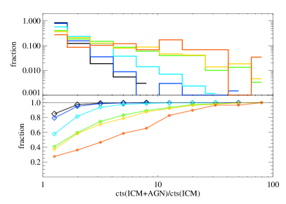
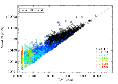
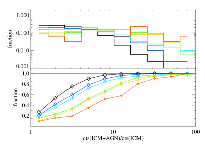
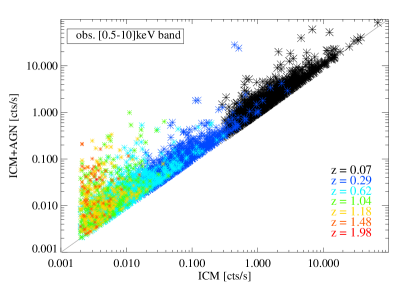
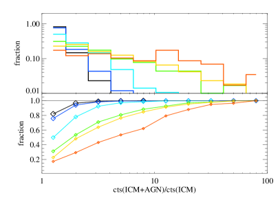
Figure 5: Count rates for ICM and ICM+AGN from eROSITA mock observations of the R500 region of clusters at various redshifts between $z=0.07$ and $\sim 2$, marked with different colours as specified in the legend. Left: AGN+ICM count rate as a function of the ICM count rate. Each data point represents one cluster. The vertical line in the SXR plot marks the minimum detection threshold of 50 photons for a 1.6 ks exposure. Right: differential (upper panel) and cumulative (lower panel) distribution of the ${\rm cts}(\mbox{ICM+AGN})/{\rm cts}(\mbox{ICM})$ ratio (see Eq. (13)) for the clusters at each redshift. Distributions are reported only when the sample includes more than 3 sources. Colours are the same as in the l.h.s. panels and the distributions are normalized to the total number of sources at each redshift. From top to bottom, the three panels refer to the observed SXR, HXR and [0.5–10] keV energy bands, and only sources with a minimum of 20 (ICM) photons in the SXR (for the assumed 10 ks exposure) are considered.

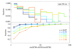
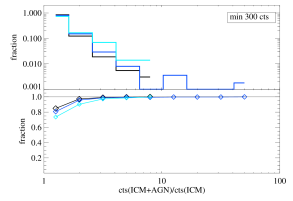
Figure 6: Same as the top-right panel in Fig. 5 (SXR), for different thresholds on the minimum ICM counts received in the SXR band: $50$ (left) and $300$ (right) photons, for the assumed 10 ks exposure.

These results for the observed SXR, HXR and [0.5–10] keV energy bands are shown in Fig. 5, for the simulated clusters catalogs at redshifts comprised between $z\sim 0$ and $z\sim 2$.

In the l.h.s. panels we show the distribution of the observed counts per second due to the sum of ICM and AGN emission versus the count rate due to the ICM only. Different colors refer to different redshifts, as in the legend. In the r.h.s. panels, we report a more quantitative representation of the ratio

$$f_{\rm cts}\equiv{\rm cts}(\mbox{ICM+AGN})/{\rm cts}(\mbox{ICM}),$$ (13)

in terms of differential (histograms; upper insets) and cumulative distribution (asterisk symbols; lower insets).

From the inspection of the upper-row panels in Fig. 5, relative to the observed SXR band, we note a trend with redshift such that the number of sources with ${\rm cts}(\mbox{ICM+AGN})/{\rm cts}(\mbox{ICM})\gtrsim 2$ (i.e. where the photon flux due to AGN is comparable to or larger than the ICM one) increases from a few percents at $z=0.07$, to 30% at $z\sim 0.6$, and to a maximum of $\sim 70\%$ at $z\sim 1.5$. This indicates that in the typical redshift-range of eROSITA observations ($z\sim 0.2\mbox{--}0.4$) only about 10–15% of the clusters will be dominated by AGN emission.

In the range $z\sim 1$–$1.2$ roughly 20%(10%) of the simulated clusters show a number of counts from AGN and ICM that is at least 5(10) times higher than that from ICM only. At high redshift, $z\sim 1.5$, this effect is very severe, and we find that, statistically, the X-ray flux coming from AGN is 10 times higher than the ICM flux for $\sim 34$% of the clusters.

The vertical line in the SXR plot marks the minimum detection threshold of 50 photons for a 1.6 ks exposure Pillepich et al. (2012), which corresponds approximately to the expected detection threshold for clusters in the eROSITA all-sky survey. With this more stringent limit, we note that only 3 sources from our simulation box would be detected at $z\sim 1$–$1.2$, and zero sources at $z\sim 1.5$, if the limit is applied to the ICM flux only. Nevertheless, the photons received from the source would comprise as well those emitted by the AGN in the cluster. If we therefore apply the same cut to the $y$-axis instead, i.e. to the AGN+ICM count rate, then one would detect 77 sources at $z\sim 1$–$1.2$ and 30 sources at $z\sim 1.5$. This means that almost all of them are actually dominated by the AGN emission.

In the central- and bottom-row panels of Fig. 5 we report analogous results for the observed HXR and [0.5–10] keV bands, where the distributions are shifting towards higher values of the $f_{\rm cts}$ ratio for increasing redshifts. The main difference is shown by the HXR case, where the power-law-like AGN emission tends to dominate over the thermal ICM one. By considering only clusters with at least 20 ICM counts in the SXR band, we note that for the faintest sources the corresponding count rates in the observed HXR can be one order of magnitude lower, that is few photons (or no photons at all) are received even in the long 10 ks exposure considered here. The fraction of sources (with at least 20 ICM counts in the SXR band) that are not detected at all in the HXR band increases with redshift, from less than $1\%$ at $z\sim 0.07$ up to $\sim 56\%$ at $z\sim 1.5$. (The only source at $z\sim 2$ is not detected in the HXR band.) With our requirements for the detection in the SXR band, much less stringent than that indicated by Pillepich et al. (2012), the HXR count rates of the observed sources indicate a contamination by AGN that is always more severe than in the SXR or [0.5–10] keV bands. In the HXR band as well, clusters can be still detected up to $z\sim 1.5$, where however $\sim 90\%(70\%)$ of the sources have a dominant AGN flux with respect to the ICM emission, $f_{\rm cts}\gtrsim 2(5)$. Interestingly, and differently from the other bands, even at $z\sim 0.07$, the photon flux due to AGN is comparable to or larger than the ICM one (i.e. $f_{\rm cts}\gtrsim 2$) already for $\sim 40\%$ of the clusters.

This is not the case for the distributions in the observed SXR and [0.5–10] keV bands, where instead the distribution is narrower at low redshifts ($z<0.6$) and strongly peaked around $f_{\rm cts}\sim 1$–$2$, whereas it significantly broadens towards higher values of $f_{\rm cts}$ with increasing redshift, and almost flattens at $z\sim 1.5$.

At redshifts $z\sim 1$–$1.5$ we therefore expect eROSITA to encounter a significant number of sources (10–30%) for which the detection of the cluster around the AGN is very challenging, with the observed X-ray flux from the latter dominating over the former by more than a factor of 10.

6.3.2 AGN-to-ICM contamination and system mass

In Fig. 6 we show the distribution of $f_{\rm cts}$ for two different lower cuts on the minimum of ICM photons received in the observed SXR energy band, namely $50$ (l.h.s. panel) and $300$ (r.h.s. panel) photons for the $10$ ks exposure.

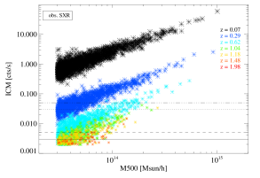
Figure 7: ICM count rate in the SXR band as a function of the cluster mass $M_{500}$, at various redshifts between $z=0.07$ and $\sim 2$, marked with different colours as specified in the legend. The horizontal lines correspond, from bottom to top, to detection limits of $30$ (solid line), $50$ (dashed line), $300$ (dotted line) and $500$ (dot-dashed line) photons for a $10\,$ks exposure.

As shown in the r.h.s. panel of Fig. 6, we expect to detect clusters with $M_{500}>3\times 10^{13}\,h^{-1}\rm{\,M_{\odot}}$ only up to redshift $z\sim 0.62$, when a detection limit of 300 photons is applied (corresponding to the limit of 50 photons for a typical 1.6 ks exposure of the planned eROSITA all-sky survey). At low-intermediate redshifts ($z\lesssim 0.6$) we still find that for the majority of the sources the AGN emission is at most comparable to that of the ICM alone, and no more than 20% of the sources have a dominant AGN emission.

For less stringent limits on the detection limit, such as 50 counts in 10 ks (l.h.s. panel in Fig. 6), also fainter sources can be observed in the SXR band and up to $z\sim 1.5$. In this case, a larger fraction of sources is dominated by the AGN emission, namely up to 30–60% of the clusters would have $f_{\rm cts}>2$ between redshifts $1$ and $1.5$.

By increasing the threshold on the SXR count rate detection we essentially aim at increasing the mass limit of the clusters that can be detected and obtain that only the brightest sources can be detected at high redshifts. Nevertheless, we note from Fig. 7 that the received ICM count rate in the SXR band correlates tightly with the system mass (here, $M_{500}$) only for the massive clusters. At lower masses, at fixed values of ${\rm cts(ICM)}$ corresponds in fact a large scatter in $M_{500}$, for all the redshift considered. In addition, given the trend in redshift of the ${\rm cts(ICM)}$-$M_{500}$ relation shown in Fig. 7, we note that the increasing threshold on the minimum ${\rm cts(ICM)}$ (horizontal lines in the Figure, corresponding to detection limits of $30$, $50$, $300$ and $500$ photons in $10\,$ks exposure, from bottom to top respectively) corresponds to an increasing mass cut of the observed clusters only at high redshifts. Instead, for $z\lesssim 0.3$, the entire mass range of the sample $M_{500}\gtrsim 3\times 10^{13}M_{\odot}$ is still observable, even though some sources with low mass and low count rate cannot be detected (for a discussion of the observational effects of this scatter, see e.g. Allen et al., 2011). We remind that Fig. 7 includes all the sources with at least 20 ICM counts detected in the SXR band, as in Fig. 5. We verified nonetheless that the presence of sources that are dominated by the AGN emission — for which the correct estimation of the ICM count rates can be therefore compromised — does not introduce any bias. By removing the AGN-dominated sources, in fact, the number of sources is reduced with a more prominent effect at high redshift, but the trends observed in Fig. 7 are preserved, making our conclusions unchanged.

For the purpose of comparison, we show in Fig. 8 the distribution of $f_{\rm cts}$, in the observed SXR band, for the subsample of clusters with $M_{500}\gtrsim 10^{14}M_{\odot}$. (As in Fig. 5, we require a minimum of 20 ICM photons in the SXR band, for the assumed 10 ks exposure.) With respect to Fig. 6, we see that the most massive clusters can be detected up to redshift $z\sim 1.2$, with a small contamination due to AGN in the majority of the cases. Nevertheless, at $z\sim 1\mbox{--}1.2$ the $f_{\rm cts}$ distribution shows a tail towards higher values, due to the large scatter, at fixed mass, in the AGN emission with respect to the ICM one. From this case, we infer that even for massive clusters, $15$–$25$% of the sources at $z\sim 1\mbox{--}1.2$ can be largely dominated by their AGN component in the observed SXR photon flux, with an AGN count rate that is at least 5 times larger than the ICM count rate ($f_{\rm cts}\gtrsim 5$).

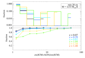
Figure 8: Same as the top-right panel in Fig. 5 (SXR energy band), for the cluster in the sample with $M_{500}\gtrsim 10^{14}M_{\odot}$. As in Fig. 5, here only sources with at least 20 counts in the SXR band (for the 10 ks exposure) are considered.

7 Summary and conclusion

In this paper we have presented a new implementation of the X-ray emission modelling from AGN sources within the Magneticum Pathfinder Simulation set. We showed that the population of AGN in the Magneticum Pathfinder Simulation statistically well reproduces the observed bolometric unabsorbed and SXR/HXR absorbed LFs up to redshift $z\sim 2$, over a large range of luminosities. As an application, we presented predictions on the eROSITA observations of AGN and ICM X-ray fluxes for a sample of galaxy clusters, in the range $0\lesssim z\lesssim 2$, quantifying the contamination due to the AGN emission w.r.t. the ICM X-ray flux.

Our main findings can be summarized as follows.

Bolometric LFs from the simulated AGN catalogs have been analysed and compared against observational data in order to evaluate the reliability of the intrinsic simulated population of SMBHs (Fig. 1) (see also Hirschmann et al., 2014). The theoretical estimation of their bolometric luminosity and the therefrom derived unabsorbed SXR and HXR luminosity (under the assumtion of the bolometric corrections by Marconi et al. (2004)) were then used to constrain in a self-consistent way the spectral parameters of the X-ray emission associated to each AGN source. In the modelling of the X-ray emission from each source, we further statistically associate to each AGN source a value for the column density of the obscuring material expected to reside in the torus surrounding the AGN, by assuming an observationally-motivated distribution of the obscurer column densities (from Buchner et al., 2014). This modelling is embedded into our PHOX photon simulator in order to derive the X-ray synthetic emission from the AGN component in the simulations (Section 4.3 and 4.3.1). The assumption of an obscuration component at the sources allowed us to test the obscured LFs in both the soft and hard X-ray energy bands (Section 5), which show a remarkable level of agreement with observational LFs for the high-luminosity tail in all the redshift bins analysed between $z=0.1$ and $z=1.2$. The simulated LFs still overpredict the observational ones at low luminosities, in both energy bands. Nevertheless, when an additional luminosity- and redshift-dependent obscuration fraction is considered, e.g. following Hasinger (2008), we find that the comparison between our results and observed LFs remarkably improves. In both energy bands, the simulated LFs decrease at low luminosities and are in overall good agreement with observed LFs by Hasinger et al. (2005), Aird et al. (2010) and Buchner et al. (2015) at almost all redshifts (see Fig. 3). However, we still note a discrepancy in the SXR LFs at $z=2.3$.

The importance of producing realistic X-ray catalogs of simulated AGN in order to compare the intrinsic population of simulated SMBHs with the statistical properties of observed AGN is also discussed in a recent study by Koulouridis et al. (2017) on the cosmo-OWLS simulations. They also include a modelling of the obscuration fraction which depends on redshift and luminosity of the AGN, showing that the AGN in the cosmo-OWLS simulations reproduce very well the observational data. In addition to LFs, Koulouridis et al. (2017) focus on the correlation function of AGN in the mock XMM-Newton X-ray catalogs and on the comparison to observed Eddington ratio distribution, finding as well a good match with observations. Differently from their work, here we include self-consistently the modelling of the AGN X-ray emission depending on the intrinsic luminosity predicted by the simulations, and assuming an observationally-based torus obscuration component for every AGN source (including both Compton-thick and unobscured objects) in the simulation.

The use of mock X-ray observations is particularly important to study the combined emission of AGN and ICM in clusters. We dedicate the second part of this analysis to explicitly studying the mock X-ray emission of AGN in simulated clusters (Section 6). This provides a prediction for the effects due to the presence of AGN on the detection of clusters, as expected from eROSITA-like observations. Differently from the study of the absorbed LFs, where we do not include any instrumental response in order to purely test our modelling of the AGN emission including the torus obscuration component, we generate complete eROSITA-like mock observations with PHOX in order to investigate the observed AGN emission in galaxy clusters. Specifically, we employ the PHOX X-ray simulator to generate eROSITA synthetic observations for a sample of galaxy clusters with masses $M_{500}>3\times 10^{13}\,h^{-1}\rm{\,M_{\odot}}$, extracted from the Magenticum Pathfinder Simulation at various redshifts between $z=0$ and $z=2$. This allows us to explore and predict the expected contamination from AGN emission to the ICM X-ray luminosity of the hosting cluster, which will be very important in future X-ray survey, especially of the high-redshift Universe, like eROSITA (Section 6.3). At low redshift ($z\lesssim 0.3$), we find that only for a small fraction of clusters ($\sim 5\mbox{--}10\%$) the observed X-ray flux from the AGN within the projected $R_{500}$ radius is comparable to or larger than the flux emitted by the whole ICM. As expected, however, this fraction increases for increasing redshifts. At redshifts $z\sim 1\mbox{--}1.5$, the majority of our clusters are faint and present a dominant AGN component in the X-ray emission. Specifically, the flux observed from AGN and ICM is more than a factor of 5 with respect to the flux from the ICM alone for 20–45% of the sources. If the observed SXR band is considered, $\sim 34\%$ of our clusters show that the AGN+ICM flux is at least 10 times higher than the flux of the ICM. This result is consistent with the intrinsic prediction from the simulated catalogs, where the central AGN source(s) alone (residing within 5% of the cluster virial radius) can emit an X-ray luminosity that is up 10 times higher than the $L_{X}$ of the whole ICM (see Fig. 4). When only the subsample of massive clusters ($M_{500}>10^{14}\,h^{-1}\rm{\,M_{\odot}}$) is considered, we find that the vast majority of them is not dominated by the AGN emission, except for 15–25% of the sources at $z\sim 1$–$1.2$.

The particular assumptions made in this analysis, for instance on the observed distribution of column densities of the torus obscurer component or on the luminosity- and redshift-dependent obscuration fraction, can also moderately impact our conclusions. We note, nevertheless, that updates to account for recent observational improvements can be easily implemented into the PHOX simulator, in future works.

Next-generation of wide-area X-ray surveys, especially those dedicated to exploring the high-$z$ Universe like eROSITA, will necessarily have to deal with the ambiguity of detecting the diffuse emission from galaxy clusters around powerful AGN sources, which might dominate the X-ray observed flux. As we showed here, simulations allow to predict the statistical occurrence of these cases. Multi-wavelenght observations can also play an important role in detecting the presence of massive clusters around X-ray AGN sources, as discussed by Green et al. (2017). Viceversa, spectroscopic followup of large number of X-ray sources detected by eROSITA (such as those planned by SDSS-V, Kollmeier et al. 2017, or 4MOST, de Jong et al. 2014) will allow AGN to be identified with high reliability. This will be crucial to investigate the role of AGN and associated feedback within BCGs and clusters up to high redshifts, where these phenomena are strictly connected to the thermodynamical and chemical evolution of the cluster itself.

Appendix A Mock eROSITA images

As an example, in Fig. 9 we report the synthetic 10 ks eROSITA image of two example clusters in the sample, one at $z=1$ and one at $z=0.62$. In particular, we show the images obtained from the combined emission of ICM and AGN sources in each cluster (l.h.s. insets in each figure) and those for the ICM only (r.h.s. insets). These are two examples of detected clusters, where the AGN emission is not dominant over the ICM. In the bottom-row panels we show the zoom onto the central region of the pointing. For comparison, we show in Fig. 10 two additional example clusters where instead the AGN contribution to the X-ray emission is dominant with respect to the ICM one. Specifically, from the zoom onto the central region, one can clearly notice the increase in the central X-ray surface brightness when the AGN emission is also included (l.h.s. insets), with respect to the images obtained only for the ICM (r.h.s. insets).

The images were obtained performing pointed observations with the standard SIXTE setup, for which the PSF is rapidly degrading (increasing) towards higher off-axis angles (see, e.g. Merloni et al., 2012), as noticeable at the edges of the pointings in the upper panels of Fig. 9. In reality, however, observations like those investigated here will be rather performed in survey (scanning) mode, which will results in an effective average PSF Half-Energy Widthof $28"$ in the soft band and $\sim 40"$ in the hard band. In the current analysis these features of the PSF do not play any major role, since we perform a pointed observation for every single cluster, which typically resides in the very central region of the FoV (see the zooms in Figs. 9 and 10).

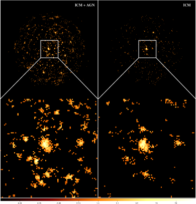
(a) $z=1$

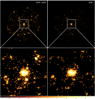
(b) $z=0.62$

Figure 9: eROSITA mock observations of two example clusters in our simulation box, one at $z=1$ (a) and one at $z=0.62$ (b). In each figure we show the emission from AGN and ICM in the cluster (left insets) and the emission from the ICM only (right insets). In the bottom row insets we show the zoom onto the central region, as marked. The pointed observations were obtained with the standard SIXTE setup, without including the background and projecting along the line of sight for the whole simulation box lenght ($500$ Mpc).

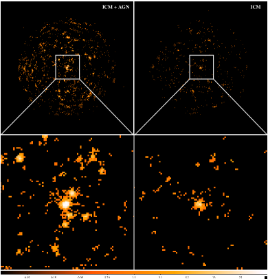
(a) $z=1$

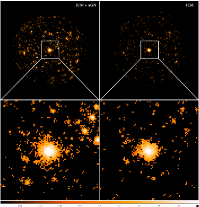
(b) $z=0.62$

Figure 10: Same as Fig. 9, for two example clusters where the X-ray emission of the AGN is dominating over the ICM one.

References

- Aird et al. (2015) Aird J., Coil A. L., Georgakakis A., Nandra K., Barro G., Pérez-González P. G., 2015, MNRAS, 451, 1892
- Aird et al. (2010) Aird J., Nandra K., Laird E. S., Georgakakis A., Ashby M. L. N., Barmby P., Coil A. L., Huang J.-S., Koekemoer A. M., Steidel C. C., Willmer C. N. A., 2010, MNRAS, 401, 2531
- Allen et al. (2011) Allen S. W., Evrard A. E., Mantz A. B., 2011, ARA&A, 49, 409
- Arnaud (1996) Arnaud K. A., 1996, in G. H. Jacoby & J. Barnes ed., Astronomical Data Analysis Software and Systems V Vol. 101 of Astronomical Society of the Pacific Conference Series, XSPEC: The First Ten Years. pp 17–+
- Assef et al. (2011) Assef R. J., Kochanek C. S., Ashby M. L. N., Brodwin M., Brown M. J. I., Cool R., Forman W., Gonzalez A. H., Hickox R. C., Jannuzi B. T., Jones C., Le Floc’h E., Moustakas J., Murray S. S., Stern D., 2011, ApJ, 728, 56
- Barai et al. (2014) Barai P., Viel M., Murante G., Gaspari M., Borgani S., 2014, MNRAS, 437, 1456
- Barger & Cowie (2005) Barger A. J., Cowie L. L., 2005, ApJ, 635, 115
- Beck et al. (2016) Beck A. M., Murante G., Arth A., Remus R.-S., Teklu A. F., Donnert J. M. F., Planelles S., Beck M. C., Förster P., Imgrund M., Dolag K., Borgani S., 2016, MNRAS, 455, 2110
- Benson et al. (2003) Benson A. J., Bower R. G., Frenk C. S., Lacey C. G., Baugh C. M., Cole S., 2003, ApJ, 599, 38
- Biffi et al. (2013) Biffi V., Dolag K., Böhringer H., 2013, MNRAS, 428, 1395
- Biffi et al. (2012) Biffi V., Dolag K., Böhringer H., Lemson G., 2012, MNRAS, 420, 3545
- Biffi et al. (2017) Biffi V., Planelles S., Borgani S., Fabjan D., Rasia E., Murante G., Tornatore L., Dolag K., Granato G. L., Gaspari M., Beck A. M., 2017, MNRAS, 468, 531
- Biffi et al. (2014) Biffi V., Sembolini F., De Petris M., Valdarnini R., Yepes G., Gottlöber S., 2014, MNRAS, 439, 588
- Biffi & Valdarnini (2015) Biffi V., Valdarnini R., 2015, MNRAS, 446, 2802
- Bongiorno & et al. (2007) Bongiorno A., et al. 2007, A&A, 472, 443
- Booth & Schaye (2009) Booth C. M., Schaye J., 2009, MNRAS, 398, 53
- Booth & Schaye (2011) Booth C. M., Schaye J., 2011, MNRAS, 413, 1158
- Boyle et al. (1993) Boyle B. J., Griffiths R. E., Shanks T., Stewart G. C., Georgantopoulos I., 1993, MNRAS, 260, 49
- Boyle et al. (2000) Boyle B. J., Shanks T., Croom S. M., Smith R. J., Miller L., Loaring N., Heymans C., 2000, MNRAS, 317, 1014
- Boyle et al. (1994) Boyle B. J., Shanks T., Georgantopoulos I., Stewart G. C., Griffiths R. E., 1994, MNRAS, 271, 639
- Buchner et al. (2015) Buchner J., Georgakakis A., Nandra K., Brightman M., Menzel M.-L., Liu Z., Hsu L.-T., Salvato M., Rangel C., Aird J., Merloni A., Ross N., 2015, ApJ, 802, 89
- Buchner et al. (2014) Buchner J., Georgakakis A., Nandra K., Hsu L., Rangel C., Brightman M., Merloni A., Salvato M., Donley J., Kocevski D., 2014, A&A, 564, A125
- Churazov et al. (2005) Churazov E., Sazonov S., Sunyaev R., Forman W., Jones C., Böhringer H., 2005, MNRAS, 363, L91
- Croom et al. (2009) Croom S. M., Richards G. T., Shanks T., Boyle B. J., Strauss M. A., Myers A. D., Nichol R. C., Pimbblet K. A., Ross N. P., Schneider D. P., Sharp R. G., Wake D. A., 2009, MNRAS, 399, 1755
- Croton et al. (2006) Croton D. J., Springel V., White S. D. M., De Lucia G., Frenk C. S., Gao L., Jenkins A., Kauffmann G., Navarro J. F., Yoshida N., 2006, MNRAS, 365, 11
- Cui et al. (2016) Cui W., Power C., Biffi V., Borgani S., Murante G., Fabjan D., Knebe A., Lewis G. F., Poole G. B., 2016, MNRAS, 456, 2566
- David et al. (2001) David L. P., Nulsen P. E. J., McNamara B. R., Forman W., Jones C., Ponman T., Robertson B., Wise M., 2001, ApJ, 557, 546
- de Jong et al. (2014) de Jong R. S., Barden S., Bellido-Tirado O., Brynnel J., Chiappini C., Depagne É., Haynes R., Johl D., Phillips D. P., Schnurr O., Schwope A. D., Walcher J., et al. 2014, in Ground-based and Airborne Instrumentation for Astronomy V Vol. 9147 of Proc. SPIE, 4MOST: 4-metre Multi-Object Spectroscopic Telescope. p. 91470M
- Degraf et al. (2010) Degraf C., Di Matteo T., Springel V., 2010, MNRAS, 402, 1927
- Degraf et al. (2011) Degraf C., Di Matteo T., Springel V., 2011, MNRAS, 413, 1383
- Dehnen & Aly (2012) Dehnen W., Aly H., 2012, MNRAS, 425, 1068
- Di Matteo et al. (2008) Di Matteo T., Colberg J., Springel V., Hernquist L., Sijacki D., 2008, ApJ, 676, 33
- Di Matteo et al. (2012) Di Matteo T., Khandai N., DeGraf C., Feng Y., Croft R. A. C., Lopez J., Springel V., 2012, ApJ, 745, L29
- Di Matteo et al. (2005) Di Matteo T., Springel V., Hernquist L., 2005, Nature, 433, 604
- Dolag et al. (2004) Dolag K., Jubelgas M., Springel V., Borgani S., Rasia E., 2004, ApJ, 606, L97
- Dolag & Stasyszyn (2009) Dolag K., Stasyszyn F., 2009, MNRAS, 398, 1678
- Dolag et al. (2005) Dolag K., Vazza F., Brunetti G., Tormen G., 2005, MNRAS, 364, 753
- Fabian (1994) Fabian A. C., 1994, ARA&A, 32, 277
- Fabian (2012) Fabian A. C., 2012, ARA&A, 50, 455
- Fabian et al. (1984) Fabian A. C., Nulsen P. E. J., Canizares C. R., 1984, Nature, 310, 733
- Fabian et al. (2003) Fabian A. C., Sanders J. S., Allen S. W., Crawford C. S., Iwasawa K., Johnstone R. M., Schmidt R. W., Taylor G. B., 2003, MNRAS, 344, L43
- Fabjan et al. (2010) Fabjan D., Borgani S., Tornatore L., Saro A., Murante G., Dolag K., 2010, MNRAS, 401, 1670
- Ferrarese & Ford (2005) Ferrarese L., Ford H., 2005, SSR, 116, 523
- Ferrarese & Merritt (2000) Ferrarese L., Merritt D., 2000, ApJ, 539, L9
- Fiore et al. (2012) Fiore F., Puccetti S., Grazian A., Menci N., Shankar F., Santini P., Piconcelli E., Koekemoer A. M., Fontana A., Boutsia K., Castellano M., Lamastra A., Malacaria C., Feruglio C., Mathur S., Miller N., Pannella M., 2012, A&A, 537, A16
- Fotopoulou et al. (2016) Fotopoulou S., Buchner J., Georgantopoulos I., Hasinger G., Salvato M., Georgakakis A., Cappelluti N., Ranalli P., Hsu L. T., Brusa M., Comastri A., Miyaji T., Nandra K., Aird J., Paltani S., 2016, A&A, 587, A142
- Gebhardt et al. (2000) Gebhardt K., Bender R., Bower G., Dressler A., Faber S. M., Filippenko A. V., Green R., Grillmair C., Ho L. C., Kormendy J., Lauer T. R., Magorrian J., Pinkney J., Richstone D., Tremaine S., 2000, ApJ, 539, L13
- Gitti et al. (2012) Gitti M., Brighenti F., McNamara B. R., 2012, Advances in Astronomy, 2012, 950641
- Green et al. (2017) Green T. S., Edge A. C., Ebeling H., Burgett W. S., Draper P. W., Kaiser N., Kudritzki R.-P., Magnier E. A., Metcalfe N., Wainscoat R. J., Waters C., 2017, MNRAS, 465, 4872
- Haardt & Madau (2001) Haardt F., Madau P., 2001, in Neumann D. M., Tran J. T. V., eds, Clusters of Galaxies and the High Redshift Universe Observed in X-rays Modelling the UV/X-ray cosmic background with CUBA
- Haas et al. (2013) Haas M. R., Schaye J., Booth C. M., Dalla Vecchia C., Springel V., Theuns T., Wiersma R. P. C., 2013, MNRAS, 435, 2931
- Hahn et al. (2015) Hahn O., Martizzi D., Wu H.-Y., Evrard A. E., Teyssier R., Wechsler R. H., 2015, ArXiv e-prints
- Hasinger (2008) Hasinger G., 2008, A&A, 490, 905
- Hasinger et al. (2005) Hasinger G., Miyaji T., Schmidt M., 2005, A&A, 441, 417
- Hirschmann et al. (2014) Hirschmann M., Dolag K., Saro A., Bachmann L., Borgani S., Burkert A., 2014, MNRAS, 442, 2304
- Hopkins et al. (2006) Hopkins P. F., Hernquist L., Cox T. J., Robertson B., Di Matteo T., Springel V., 2006, ApJ, 639, 700
- Hopkins et al. (2007) Hopkins P. F., Richards G. T., Hernquist L., 2007, ApJ, 654, 731
- Kollmeier et al. (2017) Kollmeier J. A., Zasowski G., Rix H.-W., Johns M., Anderson S. F., Drory N., Johnson J. A., Pogge R. W., Bird J. C., Blanc G. A., Brownstein J. R., Crane J. D., De Lee N. M., Klaene M. A., Kreckel K., MacDonald N., Merloni A., et al. 2017, ArXiv e-prints
- Kormendy & Ho (2013) Kormendy J., Ho L. C., 2013, ARA&A, 51, 511
- Koulouridis et al. (2017) Koulouridis E., Faccioli L., Le Brun A. M. C., Plionis M., McCarthy I. G., Pierre M., Akylas A., Georgantopoulos I., Paltani S., Lidman C., Fotopoulou S., Vignali C., Pacaud F., Ranalli P., 2017, ArXiv e-prints
- La Franca et al. (2005) La Franca F., Fiore F., Comastri A., Perola G. C., Sacchi N., Brusa M., Cocchia F., Feruglio C., Matt G., Vignali C., Carangelo N., Ciliegi P., Lamastra A., Maiolino R., Mignoli M., Molendi S., Puccetti S., 2005, ApJ, 635, 864
- Liu et al. (2017) Liu T., Tozzi P., Wang J.-X., Brandt W. N., Vignali C., Xue Y., Schneider D. P., Comastri A., et al. 2017, ApJS, 232, 8
- Maccacaro et al. (1991) Maccacaro T., della Ceca R., Gioia I. M., Morris S. L., Stocke J. T., Wolter A., 1991, ApJ, 374, 117
- Maccacaro et al. (1983) Maccacaro T., Gioia I. M., Avni Y., Giommi P., Griffiths R. E., Liebert J., Stocke J., Danziger J., 1983, ApJ, 266, L73
- Maccacaro et al. (1984) Maccacaro T., Gioia I. M., Stocke J. T., 1984, ApJ, 283, 486
- Magorrian et al. (1998) Magorrian J., Tremaine S., Richstone D., Bender R., Bower G., Dressler A., Faber S. M., Gebhardt K., Green R., Grillmair C., Kormendy J., Lauer T., 1998, AJ, 115, 2285
- Maio et al. (2013) Maio U., Dotti M., Petkova M., Perego A., Volonteri M., 2013, ApJ, 767, 37
- Marconi et al. (2004) Marconi A., Risaliti G., Gilli R., Hunt L. K., Maiolino R., Salvati M., 2004, MNRAS, 351, 169
- Martizzi et al. (2016) Martizzi D., Hahn O., Wu H.-Y., Evrard A. E., Teyssier R., Wechsler R. H., 2016, MNRAS, 459, 4408
- McCarthy et al. (2011) McCarthy I. G., Schaye J., Bower R. G., Ponman T. J., Booth C. M., Dalla Vecchia C., Springel V., 2011, MNRAS, 412, 1965
- McCarthy et al. (2010) McCarthy I. G., Schaye J., Ponman T. J., Bower R. G., Booth C. M., Dalla Vecchia C., Crain R. A., Springel V., Theuns T., Wiersma R. P. C., 2010, MNRAS, 406, 822
- McConnell & Ma (2013) McConnell N. J., Ma C.-P., 2013, ApJ, 764, 184
- McNamara et al. (2005) McNamara B. R., Nulsen P. E. J., Wise M. W., Rafferty D. A., Carilli C., Sarazin C. L., Blanton E. L., 2005, Nature, 433, 45
- McNamara et al. (2000) McNamara B. R., Wise M., Nulsen P. E. J., David L. P., Sarazin C. L., Bautz M., Markevitch M., Vikhlinin A., Forman W. R., Jones C., Harris D. E., 2000, ApJ, 534, L135
- Merloni & et al. (2014) Merloni A., et al. 2014, MNRAS, 437, 3550
- Merloni & Heinz (2008) Merloni A., Heinz S., 2008, MNRAS, 388, 1011
- Merloni et al. (2012) Merloni A., Predehl P., Becker W., Böhringer H., Boller T., Brunner H., Brusa M., German eROSITA Consortium t., 2012, ArXiv e-prints
- Page et al. (1996) Page M. J., Carrera F. J., Hasinger G., Mason K. O., McMahon R. G., Mittaz J. P. D., Barcons X., Carballo R., Gonzalez-Serrano I., Perez-Fournon I., 1996, MNRAS, 281, 579
- Peterson & Fabian (2006) Peterson J. R., Fabian A. C., 2006, Phys. Rep., 427, 1
- Peterson et al. (2001) Peterson J. R., Paerels F. B. S., Kaastra J. S., Arnaud M., Reiprich T. H., Fabian A. C., Mushotzky R. F., Jernigan J. G., Sakelliou I., 2001, A&A, 365, L104
- Pillepich et al. (2012) Pillepich A., Porciani C., Reiprich T. H., 2012, MNRAS, 422, 44
- Planelles et al. (2017) Planelles S., Fabjan D., Borgani S., Murante G., Rasia E., Biffi V., Truong N., Ragone-Figueroa C., Granato G. L., Dolag K., Pierpaoli E., Beck A. M., Steinborn L. K., Gaspari M., 2017, MNRAS, 467, 3827
- Ragagnin et al. (2017) Ragagnin A., Dolag K., Biffi V., Cadolle Bel M., Hammer N. J., Krukau A., Petkova M., Steinborn D., 2017, Astronomy and Computing, 20, 52
- Ranalli & et al. (2016) Ranalli P., et al. 2016, A&A, 590, A80
- Rasia et al. (2015) Rasia E., Borgani S., Murante G., Planelles S., Beck A. M., Biffi V., Ragone-Figueroa C., Granato G. L., Steinborn L. K., Dolag K., 2015, ApJ, 813, L17
- Richards & et al. (2006) Richards G. T., et al. 2006, AJ, 131, 2766
- Sarazin (1986) Sarazin C. L., 1986, Reviews of Modern Physics, 58, 1
- Sijacki et al. (2007) Sijacki D., Springel V., Di Matteo T., Hernquist L., 2007, MNRAS, 380, 877
- Sijacki et al. (2015) Sijacki D., Vogelsberger M., Genel S., Springel V., Torrey P., Snyder G. F., Nelson D., Hernquist L., 2015, MNRAS, 452, 575
- Silverman et al. (2008) Silverman J. D., Green P. J., Barkhouse W. A., Kim D.-W., Kim M., Wilkes B. J., Cameron R. A., Hasinger G., Jannuzi B. T., Smith M. G., Smith P. S., Tananbaum H., 2008, ApJ, 679, 118
- Simpson (2005) Simpson C., 2005, MNRAS, 360, 565
- Smith et al. (2001) Smith R. K., Brickhouse N. S., Liedahl D. A., Raymond J. C., 2001, ApJ, 556, L91
- Springel (2005) Springel V., 2005, MNRAS, 364, 1105
- Springel et al. (2005) Springel V., Di Matteo T., Hernquist L., 2005, MNRAS, 361, 776
- Springel & Hernquist (2002) Springel V., Hernquist L., 2002, MNRAS, 333, 649
- Springel & Hernquist (2003) Springel V., Hernquist L., 2003, MNRAS, 339, 289
- Steinborn et al. (2016) Steinborn L. K., Dolag K., Comerford J. M., Hirschmann M., Remus R.-S., Teklu A. F., 2016, MNRAS, 458, 1013
- Steinborn et al. (2015) Steinborn L. K., Dolag K., Hirschmann M., Prieto M. A., Remus R.-S., 2015, MNRAS, 448, 1504
- Tornatore et al. (2007) Tornatore L., Borgani S., Dolag K., Matteucci F., 2007, MNRAS, 382, 1050
- Tornatore et al. (2003) Tornatore L., Borgani S., Springel V., Matteucci F., Menci N., Murante G., 2003, MNRAS, 342, 1025
- Tremaine et al. (2002) Tremaine S., Gebhardt K., Bender R., Bower G., Dressler A., Faber S. M., Filippenko A. V., Green R., Grillmair C., Ho L. C., Kormendy J., Lauer T. R., Magorrian J., Pinkney J., Richstone D., 2002, ApJ, 574, 740
- Ueda et al. (2014) Ueda Y., Akiyama M., Hasinger G., Miyaji T., Watson M. G., 2014, ApJ, 786, 104
- Ueda et al. (2003) Ueda Y., Akiyama M., Ohta K., Miyaji T., 2003, ApJ, 598, 886
- Vogelsberger et al. (2017) Vogelsberger M., Marinacci F., Torrey P., Genel S., Springel V., Weinberger R., Pakmor R., Hernquist L., Naiman J., Pillepich A., Nelson D., 2017, ArXiv e-prints
- Voit & Donahue (2005) Voit G. M., Donahue M., 2005, ApJ, 634, 955
- Wiersma et al. (2009) Wiersma R. P. C., Schaye J., Smith B. D., 2009, MNRAS, 393, 99
- Wolf et al. (2003) Wolf C., Meisenheimer K., Rix H.-W., Borch A., Dye S., Kleinheinrich M., 2003, A&A, 401, 73
- Zdziarski et al. (2000) Zdziarski A. A., Poutanen J., Johnson W. N., 2000, ApJ, 542, 703