Photodissociation of CS from Excited Rovibrational Levels

Abstract

Accurate photodissociation cross sections have been computed for transitions from the $\text{X}\ ^{1}\Sigma^{+}$ ground electronic state of CS to six low-lying excited electronic states. New ab initio potential curves and transition dipole moment functions have been obtained for these computations using the multi-reference configuration interaction approach with the Davidson correction (MRCI+Q) and aug-cc-pV6Z basis sets. State-resolved cross sections have been computed for transitions from nearly the full range of rovibrational levels of the $\text{X}\ ^{1}\Sigma^{+}$ state and for photon wavelengths ranging from 500 Å to threshold. Destruction of CS via predissociation in highly excited electronic states originating from the rovibrational ground state is found to be unimportant. Photodissociation cross sections are presented for temperatures in the range between 1000 K and 10,000 K, where a Boltzmann distribution of initial rovibrational levels is assumed. Applications of the current computations to various astrophysical environments are briefly discussed focusing on photodissociation rates due to the standard interstellar and blackbody radiation fields.

1 Introduction

CS is a molecule of great astrophysical interest. It is also one of the most abundant sulfur-bearing compounds in interstellar clouds and is found in a variety of astrophysical objects including star-forming regions (Walker et al., 1986), protostellar envelopes (Herpin et al., 2012), dense interstellar clouds (Hasegawa et al., 1984; Hayashi et al., 1985; Destree, Snow, & Black, 2009), carbon-rich stars (Bregman et al., 1978; Ridgway et al., 1997; Tenenbaum et al., 2010), oxygen-rich stars (Ziurys et al., 2007; Tenenbaum et al., 2010), planetary nebulae (Edwards & Ziurys, 2014), and comets (Smith et al., 1980; Jackson et al., 1982; Canaves et al., 2007).

Photodissociation is an important mechanism for the destruction of molecules in environments with an intense radiation field, so accurate photodissociation rates are necessary to estimate the abundance of CS. Heays et al. (2017) presented photodissociation cross sections and photorates for CS using previous estimates (van Dishoeck, 1988) applying measured wavelengths for transitions to the B$~{}^{1}\Sigma^{+}$ (or 3$~{}^{1}\Sigma^{+}$) from the ground state (Stark et al., 1987) and vertical excitation energies of higher states (Bruna et al., 1975). However, comprehensive photodissociation cross sections are needed to compute photorates in many environments. In response, we have calculated photodissociation cross sections for the CS molecule for several electronic transitions from a wide range of initial rovibrational levels. Photodissociation cross sections for transitions from the $\text{X}\ ^{1}\Sigma^{+}$ electronic ground state to the $\text{A}\ ^{1}\Pi$, $\text{A}^{\prime}\ {}^{1}\Sigma^{+}$($2\ ^{1}\Sigma^{+}$), $2\ ^{1}\Pi$, $3\ ^{1}\Pi$, $\text{B}\ ^{1}\Sigma^{+}$($3\ ^{1}\Sigma^{+}$), and $4\ ^{1}\Pi$ electronic states are studied here. Calculations have been performed for transitions from $14,908$ initial bound rovibrational levels $v^{\prime\prime},J^{\prime\prime}$ of the X state. We also explore predissociation out of the $3\ ^{1}\Pi$, $\text{B}\ ^{1}\Sigma^{+}$, and $4\ ^{1}\Pi$ excited electronic states.

The present cross section calculations are performed using quantum-mechanical techniques. Applications of the cross sections to environments appropriate for local thermodynamic equilibrium (LTE) conditions are included, where a Boltzmann distribution of initial rovibrational levels is assumed. Photodissociation rates are computed for the standard interstellar radiation field (ISRF) and for blackbody radiation fields at a wide range of temperatures.

The layout of this paper is as follows. An overview of the theory of molecular photodissociation and the adopted molecular data is presented in section 2. In section 3, the computed state-resolved cross sections, LTE cross sections, and photodissociation rates are discussed. Finally, in section 4, conclusions are drawn from our work. Atomic units are used throughout unless otherwise specified.

2 Theory and Calculations

2.1 Potential Curves and Transition Dipole Moments

In a similar manner to our recent molecular structure work on the SiO molecule (Forrey et al., 2016; Cairnie et al., 2017), which is iso-electronic to CS, the potential energy curves and transition dipole matrix (TDM) elements for several of the low-lying electronic states are calculated. We use a state-averaged-multi-configuration-self-consistent-field (SA-MCSCF) approach, followed by multi-reference configuration interaction (MRCI) calculations together with the Davidson correction (MRCI+Q; Helgaker et al., 2000). The SA-MCSCF method is used as the reference wave function for the MRCI calculations.

Potential energy curves (PECs) and TDMs as a function of internuclear distance $R$ are calculated starting from a bond separation of $R=1.8$ Bohr extending out to $R=12$ Bohr. At bond distances beyond this value we use a multipole expansion, detailed below, to represent the long-range part of the potentials. The basis sets used in our work are the augmented correlation consistent polarized sextuplet (aug-cc-pV6Z (AV6Z)) Gaussian basis sets. The use of such large basis sets is well known to recover 98% of the electron correlation effects in molecular structure calculations (Helgaker et al., 2000). All the PEC and TDM calculations for the CS molecule were performed with the quantum chemistry program package MOLPRO 2015.1 (Werner, H.-J. et al., 2015), running on parallel architectures.

Table 1: The permanent dipole moment $\mu_{X}$ for the $\text{X}\ ^{1}\Sigma^{+}$ ground state of the CS molecule at $2.9$ $a_{0}$/1.5346 Å, a value near equilibrium, compared with experiment, SCF, CAS-CI, MRCI+Q, and MCSCF theoretical calculations.

CS Ground State	Method	Basis Set	μ_X (Debye)	Δ (%)
$\text{X}\ ^{1}\Sigma^{+}$	EXPTa	$\cdots$	1.958 ±0.005	$\cdots$
$\cdots$	MRCI+Qb	aug-cc-pV6Z	2.042	+4.3%
$\cdots$	MCSCFc	aug-cc-pV6Z	2.179	+11%
$\cdots$	CAS-CId	double-zeta + polarization (DZP)	2.147	+9.7%
$\cdots$	SCFe	double-zeta + polarization (DZP)	1.783	-8.9%
$\cdots$	CIf	double-zeta (DZ)	2.350	+20%
$\cdots$	HFg	double-zeta (DZ)	1.650	-16%

For molecules with degenerate symmetry, an Abelian subgroup is required to be used in MOLPRO. For a diatomic molecule like CS with C_∞v symmetry, it will be substituted by C_2v symmetry with the order of irreducible representations being ($A_{1}$, $B_{1}$, $B_{2}$, $A_{2}$). When symmetry is reduced from C_∞v to C_2v, the correlating relationships are $\sigma\rightarrow a_{1}$, $\pi\rightarrow$ ($b_{1}$, $b_{2}$), and $\delta\rightarrow$ ($a_{1}$, $a_{2}$). In order to take account of short-range interactions, we employed the non-relativistic state-averaged complete active-space-self-consistent-field (SA-CASSCF)/MRCI method available within the MOLPRO (Werner, H.-J. et al., 2012, 2015) quantum chemistry suite of codes.

Table 2: Equilibrium Bond distance $R_{e}$ (Å) and Dissociation Energies $D_{e}$ (eV) for the $\text{X}\ ^{1}\Sigma^{+}$, $\text{A${}^{\prime}$}\ ^{1}\Sigma^{+}$ and $\text{A}\ ^{1}\Pi$ Molecular States of CS from the Present MRCI+Q Calculations Compared to Other Theoretical and Experimental Results

Molecular State	Method	Basis Set	$R_{e}$/Å	$D_{e}$/(eV)
$\text{X}\ ^{1}\Sigma^{+}$	MRCI + Qa	aug-cc-pV6Z (AV6Z)	1.5314	7.6113
	MRCI + Qb	aug-cc-pwCV5Z (ACV5Z)	1.5346	7.3851
	MRCI + Qc	aug-cc-pV6Z (AV6Z)	1.5346	$\cdots$
	MRCI + Q + cv + dkd	aug-cc-pV6Z (AV6Z)	1.5377	$\cdots$
	CCSD(T) + cv + dk + 56e	aug-cc-pV6Z (AV6Z)	1.5387	$\cdots$
	MRCIf	aug-cc-pC5VZ (C) + aug-cc-pV5Z (S)	1.5334	7.3436
	M-S-APEFg	aug-cc-pC5VZ (C) + aug-cc-pV5Z (S)	1.5403	7.3436
	HF/DF-B3LYPh	aug-cc-pVTZ	1.5360	7.0644
	EXPTi	$\cdots$	1.5349	$\cdots$
	EXPTj	$\cdots$	1.5350	$\cdots$
	EXPTk	$\cdots$	1.5349	7.3530 $\pm$ 0.025
	MORSE/RKRl	$\cdots$	1.5349	7.4391
A${}^{\prime}\ {}^{1}\Sigma^{+}(\text{2}\ ^{1}\Sigma^{+}$)	MRCI + Qa	aug-cc-pV6Z (AV6Z)	1.9443	0.4558
	MRCI + Qb	aug-cc-pwCV5Z (ACV5Z)	1.9399	0.4253
	MRCI + Qc	aug-cc-pV6Z (AV6Z)	1.9399	$\cdots$
	EXPTi	$\cdots$	1.9440	$\cdots$
	EXPTj	$\cdots$	1.9440	$\cdots$
$\text{A}\ ^{1}\Pi$	MRCI + Qa	aug-cc-pV6Z (AV6Z)	1.5622	2.7333
	MRCI + Qb	aug-cc-pwCV5Z (ACV5Z)	1.5676	2.6637
	MRCI + Qc	aug-cc-pV6Z (AV6Z)	1.5676	$\cdots$
	MRCI + Q + cv + dkd	aug-cc-pV6Z (AV6Z)	1.5690	$\cdots$
	EXPTi	$\cdots$	1.5739	$\cdots$
	EXPTj	$\cdots$	1.5660	$\cdots$

Note. — The data are given in units conventional to quantum chemistry with $1~{}\text{\AA}=10^{-10}~{}\text{m}$ and $0.529177~{}\text{\AA}\approx 1~{}a_{0}$. The conversion factor $1.239842\times 10^{-4}~{}\text{eV}=1~{}\text{cm}^{-1}$ is also used.

For the CS molecule, eight molecular orbitals (MOs) are put into the active space, including four $a_{1}$, two $b_{1}$ and two $b_{2}$ symmetry MOs which correspond to the $3s3p$ shell of sulfur and $2s2p$ shell of carbon. The rest of the electrons in the CS molecule are put into closed-shell orbitals, including four $a_{1}$, one $b_{1}$ and one $b_{2}$ symmetry MOs. The molecular orbitals for the MRCI procedure were obtained using the SA-MCSF method, for which we carried out the averaging processes on the lowest three ${}^{1}\Sigma^{+}$ (${}^{1}A_{1}$), three ${}^{1}\Pi$ (${}^{1}B_{1}$), three ${}^{3}\Sigma^{+}$ (${}^{3}A_{1}$), three ${}^{3}\Pi$ (${}^{3}B_{1}$), two ${}^{1}\Delta$ (${}^{1}A_{2}$) and two ${}^{3}\Delta$ (${}^{3}A_{2}$) molecular states. The fourteen MOs ($8a_{1}$, 3b₁, 3b₂, $0a_{2}$), i.e. (8,3,3,0), were then used to perform all the PEC and TDM calculations for the electronic states of interest in the MRCI+Q approximation. Table 1 compares theoretical results for the permanent dipole moment $\mu_{X}$ of the $\text{X}\ ^{1}\Sigma^{+}$ ground state at various levels of approximation with experiment to demonstrate the accuracy of the MRCI+Q approximation applied here. As can be seen from Table 1 our MRCI+Q results for the permanent dipole moment of CS, for the ground state, at the equilibrium geometry, are within 4% of the experimental value (Winnewisser & Cook, 1968). Table 2 compares the equilibrium distance $R_{e}$ (Å) and the dissociation energy $D_{e}$ (eV) at various level of approximation for the $\text{X}~{}^{1}\Sigma^{+}$, $\text{A}^{\prime}\ {}^{1}\Sigma^{+}$, and A$~{}^{1}\Pi$ states of CS. We note that for the $\text{X}\ ^{1}\Sigma^{+}$ ground state, the early experimental work of Crawford & Shurcliff (1934) determined values $R_{e}$ = 1.2851 Å and $D_{e}$ (eV) = 7.752 eV, in less favorable agreement with our present ab initio work or that of other high level molecular structure calculations. As shown in Table 2 the use of polarized-core-valence basis sets by Li et al. (2013) provides spectroscopically accurate results for $R_{e}$ (Å) and $D_{e}$ (eV), respectively, being within 0.03 pm and 0.032 eV compared with the available experiment. We find that our TDMs differ slightly in magnitude but agree in trend with those presented by Li et al. (2013) on the range they are computed.

Beyond a bond separation of $R=12$ Bohr, a multipole expansion is smoothly fitted to the PECs and TDMs up to $R=100$ Bohr. For the PECs this has the form

$$V(R)=-\frac{C_{5}}{R^{5}}-\frac{C_{6}}{R^{6}}\,,$$ (1)

where $C_{5}$ and $C_{6}$ are coefficients for each electronic state shown in subsection 2.1. For $R<R_{\textrm{min}}$, down to a bond length of $1.5\ \text{a}_{0}$, a short-range interaction potential of the form $V(R)=A\exp(-BR)+C$ was fitted to the ab initio potential curves.

A method to estimate the value of the quadrupole-quadrupole coefficient $C_{5}$ for an electronic state of a diatomic molecule like CS is given by Chang (1967). In order to compute the long-range dispersion coefficient $C_{6}$, the London formula

$$C_{6}=\frac{3}{2}\frac{\cal{I_{\text{C}}I_{\text{S}}}}{\cal{[I_{\text{C}}+I_{\text{S}}]}}\alpha_{\text{C}}\alpha_{\text{S}}$$ (2)

is applied, where $\alpha$ is the dipole polarizability and $\cal{I}$ is the ionization energy of each of the atoms in a given atomic state. The ionization energies are taken from the NIST Atomic Spectra Database (Kramida et al., 2016). For the sulfur atom, the dipole polarizabilities of $\alpha_{\text{S}}=18.8$ and $\alpha_{\text{S}}=19.5$, respectively, are used for the ground state $3s^{2}3p^{4}\ {}^{3}P$ and the excited state $3s^{2}3p^{4}\ {}^{1}D$ (Mukherjee & Ohno, 1989). For the ground state $2s^{2}2p^{2}\ {}^{3}P$ of atomic carbon, a dipole polarizability of $\alpha_{\text{C}}=10.39$ is used (Miller & Kelly, 1972). An estimated value of $\alpha_{\text{C}}=10.78$ is used for the excited state $2s^{2}2p^{2}\ {}^{1}D$ of carbon: this value was obtained by scaling the ground state polarizability to match the ratio of the ${}^{3}P$ and ${}^{1}D$ polarizabilities of sulfur.

Table 3: CS Electronic States

Molecular		Separated Atom									United Atom
State		Atomic State		Energy (eV)		Energy (eV)		$C_{5}$	$C_{6}$		State
X   +	${}^{1}\Sigma^{+}$		S(3s^23p^4 ^3P)	0.0	0.0	27.34	58.02	$3d^{2}4s^{2}\ a~{}^{1}D$
A   +	${}^{1}\Pi$		S(3s^23p^4 ^3P)	0.0	7.95(-4)	0.0	58.02	$3d^{2}4s^{2}\ a~{}^{1}D$
A′   +	${}^{1}\Sigma^{+}$		S(3s^23p^4 ^3P)	0.0	1.14(-3)	0.0	58.02	$3d^{2}4s^{2}\ a~{}^{1}G$
2   +	${}^{1}\Pi$		S(3s^23p^4 ^3P)	0.0	6.52(-4)	-18.23	58.02	$3d^{2}4s^{2}\ a~{}^{1}G$
B   +	${}^{1}\Sigma^{+}$		S(3s^23p^4 ^1D)	2.3812287	2.38172	27.26	55.56	$3d^{3}4s\ b~{}^{1}G$
3   +	${}^{1}\Pi$		S(3s^23p^4 ^1D)	2.3812287	2.38652	10.06	55.56	$3d^{3}4s\ b~{}^{1}G$
4   +	${}^{1}\Pi$		S(3s^23p^4 ^1D)	2.3812287	2.39969	-11.81	55.56	$3d^{3}4s\ a~{}^{1}H$
+

The potentials for the excited states of the CS molecule were shifted so that the asymptotic energies as $R\rightarrow\infty$ agree with the separated atom energy differences found in the NIST Atomic Spectra Database (Kramida et al., 2016) shown in subsection 2.1. Except for the 4 ${}^{1}\Pi$ state, shifts are less than $\sim$5 meV indicating the reliability of the MRCI+Q calculations within the uncertainty of the estimated dispersion coefficients. The potential curves for CS are shown in Figure 1.

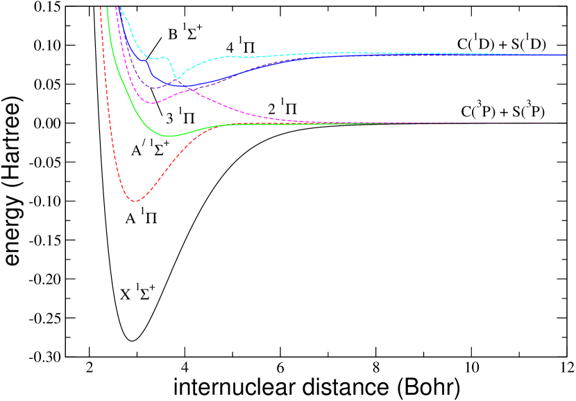
Figure 1: Potential energy curves for each considered CS molecular state.

The TDMs for the CS molecule are similarly extended to long and short-range internuclear bond distances. For $R>R_{\textrm{max}}$ a functional fit of the form $D(R)=a\exp(-bR)+c$ is applied, while in the short-range $R<R_{\textrm{min}}$ a quadratic fit of the form $D(R)=a^{\prime}R^{2}+b^{\prime}R+c^{\prime}$ is adopted. We deduce from the atomic states of C and S that the long-range $R\to\infty$ limit of each TDM is zero. Similarly, the united-atom limit (which is the Ti atom) as $R\to 0$ of each TDM is zero as well (see Table 2.1). The TDMs are shown in Figure 2.

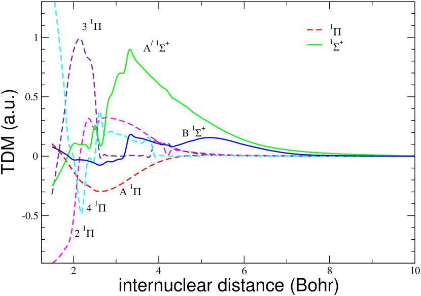
Figure 2: Transition dipole moments for transitions from the ground state to each CS excited state.

The wave functions of the bound rovibrational levels are computed by solving the radial Schrödinger equation for nuclear motion on the $\text{X}\ ^{1}\Sigma^{+}$ potential curve. The wave functions are obtained numerically using the standard Numerov method (Cooley, 1961; Johnson, 1977) with a step size of $0.001$ Bohr. We find 85 vibrational levels with a total of 14,908 rovibrational levels. This covers nearly the full range of rovibrational levels in the $\text{X}\ ^{1}\Sigma^{+}$ state.

2.2 The Photodissociation Cross Section

Here, we present a brief overview of the state-resolved photodissociation cross section calculation; further details are given in previous work (Miyake et al., 2011). In units of cm², the state-resolved cross section for a bound-free transition from initial rovibrational level $v^{\prime\prime}J^{\prime\prime}$ is

$$\sigma_{v^{\prime\prime}J^{\prime\prime}}(E_{ph})=2.689\times 10^{-18}E_{ph}g\sum_{J^{\prime}}\left(\frac{1}{2J^{\prime\prime}+1}S_{J^{\prime}}|D_{k^{\prime}J^{\prime},v^{\prime\prime}J^{\prime\prime}}|^{2}\right)$$ (3)

(Kirby & van Dishoeck, 1988) where $k^{\prime}J^{\prime}$ are the continuum states of the final electronic state. The Hönl-London factors, $S_{J^{\prime}}(J^{\prime\prime})$ (Watson, 2008), are expressed for a $\Sigma\leftarrow\Sigma$ electronic transition as

$$S_{J^{\prime}}(J^{\prime\prime})=\begin{cases}J^{\prime\prime},&J^{\prime}=J^{\prime\prime}-1\phantom{0}\phantom{0}(\textrm{P-branch})\\ J^{\prime\prime}+1,&J^{\prime}=J^{\prime\prime}+1\phantom{0}\phantom{0}(\textrm{R-branch})\,,\end{cases}$$ (4)

and for a $\Pi\leftarrow\Sigma$ transition as

$$S_{J^{\prime}}(J^{\prime\prime})=\begin{cases}(J^{\prime\prime}-1)/2,&J^{\prime}=J^{\prime\prime}-1\phantom{0}\phantom{0}(\textrm{P-branch})\\ (2J^{\prime\prime}+1)/2,&J^{\prime}=J^{\prime\prime}\phantom{0}\phantom{0}(\textrm{Q-branch})\\ (J^{\prime\prime}+2)/2,&J^{\prime}=J^{\prime\prime}+1\phantom{0}\phantom{0}(\textrm{R-branch})\,.\end{cases}$$ (5)

The matrix element of the electric TDM for absorption from $v^{\prime\prime}J^{\prime\prime}$ to the continuum $k^{\prime}J^{\prime}$ is

$$D_{k^{\prime}J^{\prime},v^{\prime\prime}J^{\prime\prime}}=\langle\chi_{k^{\prime}J^{\prime}}(R)|D(R)|\chi_{v^{\prime\prime}J^{\prime\prime}}(R)\rangle\,,$$ (6)

with the integration taken over $R$ where $D(R)$ is the appropriate TDM function. The bound rovibrational wave functions $\chi_{v^{\prime\prime}J^{\prime\prime}}$ and continuum wave functions $\chi_{k^{\prime}J^{\prime}}(R)$ are computed using the standard Numerov method with a step size of $0.001$ Bohr. They are normalized such that they behave asymptotically as

$$\chi_{k^{\prime}J^{\prime}}(R)\sim\sin\left(k^{\prime}R-\frac{\pi}{2}J^{\prime}+\eta_{J^{\prime}}\right)\ ,$$ (7)

where $\eta_{J^{\prime}}$ is the single-channel phase shift of the upper electronic state. Finally, the degeneracy factor $g$ is given by

$$g=\frac{2-\delta_{0,\Lambda^{\prime}+\Lambda^{\prime\prime}}}{2-\delta_{0,\Lambda^{\prime\prime}}}\,,$$ (8)

where $\Lambda^{\prime}$ and $\Lambda^{\prime\prime}$ are the angular momenta projected along the nuclear axis for the final and initial electronic states, respectively.

Predissociation is also possible through an intermediate transition to a bound level of an excited state. In units of cm², the predissociation cross section is

$$\sigma=8.85\times 10^{-22}\lambda^{2}x_{\ell}f_{u\ell}\eta^{d}$$ (9)

(Heays et al., 2017), where $\lambda$ is the photon wavelength in Å and $f_{u\ell}$ is the oscillator strength of the transition from lower state $\ell$ to upper state $u$. We approximate the ground-state fractional population $x_{\ell}$ and the upper level tunneling probability $\eta^{d}$ to both be 1 to give an upper limit to the predissociation cross section.

2.3 LTE Cross Sections

In LTE, a Boltzmann population distribution is assumed for the rovibrational levels in the electronic ground state. The total quantum-mechanical photodissociation cross section as a function of both temperature $T$ and wavelength $\lambda$ is

$$\sigma(\lambda,T)=\frac{\sum_{v^{\prime\prime}}\sum_{J^{\prime\prime}}g_{iv^{\prime\prime}J^{\prime\prime}}\exp[-(E_{00}-E_{v^{\prime\prime}J^{\prime\prime}})/k_{b}T]\sigma_{v^{\prime\prime}J^{\prime\prime}}}{\sum_{v^{\prime\prime}}\sum_{J^{\prime\prime}}g_{iv^{\prime\prime}J^{\prime\prime}}\exp[-(E_{00}-E_{v^{\prime\prime}J^{\prime\prime}})/k_{b}T]}\,,$$ (10)

where $g_{iv^{\prime\prime}J^{\prime\prime}}=2J^{\prime\prime}+1$ is the otal statistical weight, $E_{v^{\prime\prime}J^{\prime\prime}}$ is the magnitude of the binding energy of the rovibrational level $v^{\prime\prime}J^{\prime\prime}$, and $k_{b}$ is the Boltzmann constant. The denominator is the rovibrational partition function.

2.4 Photodissociation Rates

The photodissociation rate for a molecule in an ultraviolet radiation field is given by

$$k=\int\sigma(\lambda)I(\lambda)\,d\lambda\,,$$ (11)

where $\sigma(\lambda)$ is the photodissociation cross section and $I(\lambda)$ is the photon radiation intensity summed over all incident angles. The photon radiation intensity emitted by a blackbody with temperature $T$ is

$$I(\lambda,T)=\frac{8\pi c/\lambda^{4}}{\exp(hc/k_{b}T\lambda)-1}$$ (12)

where $h$ is the Planck constant and $c$ is the speed of light.

We also compute the photodissociation rate in the unattenuated ISRF, as given by Draine (1978), but modified for $\lambda>2000$ Å by Heays et al. (2017), using Eq. (11). In an interstellar cloud the radiation field is attenuated by dust reducing the photodissociation rate as a function of depth into the cloud, or parameterized as the visual extinction $A_{\rm V}$. Assuming a plane-parallel, semi-infinite slab, with both sides of the cloud exposed isotropically to the ISRF, we applied the radiative transfer code of Roberge et al. (1991) to compute the photodissociation rate as a function of $A_{\rm V}$ and fit the rate to the forms

$$k(A_{\rm V})=a_{1}\exp{(-a_{2}A_{\rm V}+a_{3}A_{\rm V}^{2})},$$ (13)

$$k(A_{\rm V})=a_{4}E_{2}(a_{5}A_{\rm V}),$$ (14)

where $E_{2}$ is the second-order exponential integral. The grain model of Draine & Lee (1984) that was adopted corresponds to the galactic average of the total-to-selective extinction $R_{\rm V}=3.1$.

3 Results and Discussion

3.1 State-resolved Cross Sections

State-resolved photodissociation cross sections have been computed for transitions from 14,908 initial rovibrational levels in the $\text{X}\ ^{1}\Sigma^{+}$ ground electronic state to the six considered excited electronic states. Cross sections are computed for photons with wavelengths starting at 500 Å up to at most 50,000 Å in 1 Å increments, typically stopping at the relevant threshold. A smaller wavelength step size is used near thresholds to resolve appropriate resonances. In Figure 3, a comparison of the state-resolved cross sections from the ground rovibrational level $v^{\prime\prime},J^{\prime\prime}=0,0$ for each transition is shown. The $2\ ^{1}\Pi$ and $\text{A}^{\prime}\ {}^{1}\Sigma^{+}$ ($2\ ^{1}\Sigma^{+}$) transitions have the dominant cross sections from the ground rovibrational level, while the transition to the $\text{A}\ ^{1}\Pi$ state makes very little contribution. The behavior of the current cross sections are significantly different from those adopted in Heays et al. (2017).

Predissociation is possible following bound-bound transitions to the B ${}^{1}\Sigma^{+}$, 3 ${}^{1}\Pi$, and 4 ${}^{1}\Pi$ states. Estimates of predissociation cross sections are computed for transitions to a wide range of bound rovibrational levels. Cross sections for transitions from $v^{\prime\prime},J^{\prime\prime}=0,0$ are shown in Figure 3 computed using Equation (9). We find that the line cross sections due to predissociation are much smaller than the direct cross sections for the 4 ${}^{1}\Pi$ state. However, while predissociation through the B ${}^{1}\Sigma^{+}$ and 3 ${}^{1}\Pi$ states give cross sections comparable to those of their direct continuum cross sections, the continuum cross section for the 2 ${}^{1}\Pi$ dominates the predissociation lines by more than an order of magnitude over the relevant wavelength range. Predissociation does not appear to be important for the photodestruction of CS and is therefore not considered further.

The $\text{A}^{\prime}\ {}^{1}\Sigma^{+}\leftarrow$ X$~{}^{1}\Sigma^{+}$ transition generally has large state-resolved cross sections; so a sampling of cross sections are displayed in Figure 4. Cross sections are plotted for several rotational levels of the ground vibrational level $v^{\prime\prime}=0$, and for several vibrational levels at their respective lowest rotational level, $J^{\prime\prime}=0$. State-resolved cross sections for the other five electronic transitions have also been computed (not shown).

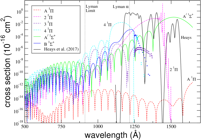
Figure 3: Comparison of CS state-resolved cross sections for transitions from the ground rovibrational level $v^{\prime\prime},J^{\prime\prime}=0,0$. The CS cross section estimate of van Dishoeck (1988), as adopted in Heays et al. (2017), is shown for comparison. Continuum cross sections (solid lines); predissociation (points) longward of $\sim$1250 Å.

Figure 4: A sample of CS state-resolved cross sections for the A${}^{\prime}\ {}^{1}\Sigma^{+}\leftarrow\text{X}\ ^{1}\Sigma^{+}$ photodissociation transition. Transitions from initial rovibrational levels (a) where $J^{\prime\prime}=0$ and (b) where $v^{\prime\prime}=0$ are shown.

3.2 LTE Cross Sections

LTE cross sections have been computed for each transition using the state-resolved cross sections from 1000 K to 10,000 K in 1000 K intervals. A comparison of LTE cross sections for each transition as a function of photon wavelength at 3000 K is displayed in Figure 5. The $\text{A}^{\prime}\ {}^{1}\Sigma^{+}\leftarrow$ X$~{}^{1}\Sigma^{+}$ transition is the dominant transition at longer wavelengths, while the $4\ ^{1}\Pi\leftarrow$ X$~{}^{1}\Sigma^{+}$ transition dominates for short wavelengths. Since the $\text{A}^{\prime}\ {}^{1}\Sigma^{+}\leftarrow$ X$~{}^{1}\Sigma^{+}$ transition is dominant for the majority of wavelengths, LTE cross sections for this transition at several temperatures are shown in Figure 6.

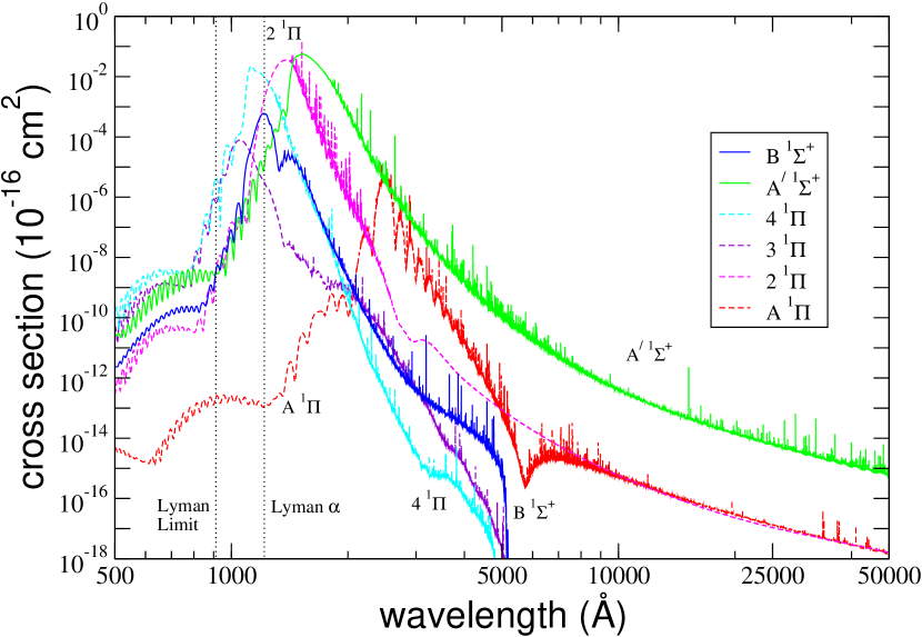
Figure 5: CS LTE cross sections at 3000 K for each of the six considered photodissociation transitions.

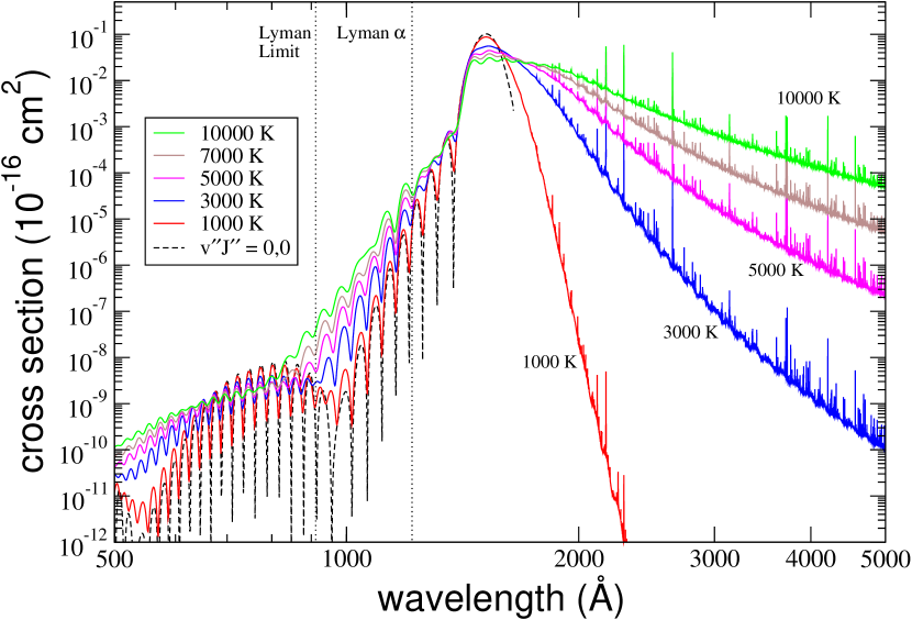
Figure 6: LTE cross sections for various kinetic temperatures for the $\text{A}^{\prime}\ {}^{1}\Sigma^{+}\leftarrow\text{X}\ ^{1}\Sigma^{+}$ transition of CS. The $v^{\prime\prime},J^{\prime\prime}=0,0$ state-resolved cross section is included as well for comparison.

3.3 Photodissociation Rates

Photodissociation rates for transitions from $v^{\prime\prime},J^{\prime\prime}=0,0$ for all six electronic transitions have been computed for the unattenuated ISRF and for the attenuated ISRF into interstellar clouds with total visual extinction. These values are listed and compared with those of Heays et al. (2017) and the UMIST compilation (McElroy et al., 2013) in Table (4). We consider fiducial diffuse and dense clouds with total visual extinctions of $A_{\rm V}$ = 1 and 20, respectively. Consistent with the cross section magnitudes, the ISRF photodissociation rates are dominated by the A${}^{\prime}~{}^{1}\Sigma^{+}\leftarrow$ X$~{}^{1}\Sigma^{+}$ and 2 ${}^{1}\Pi\leftarrow$ X$~{}^{1}\Sigma^{+}$ transitions, which leave the two atoms in their ground states. However, about 10% of the photodissociation yield results in both C and S in their ${}^{1}D$ metastable states through the 4 ${}^{1}\Pi\leftarrow$ X$~{}^{1}\Sigma^{+}$ transition. Using reliable CS photodissociation cross sections, the current unattenuated ISRF rates are about a factor of $\sim$2.5-3 smaller than the estimates adopted by Heays et al. (2017) and McElroy et al. (2013).

Table 4: Interstellar CS Photodissociation Rate Fits

. Source ISRF Dense Cloud Diffuse Cloud Products $k$(s^-1) $a_{1}$(s^-1) $a_{2}$ $a_{1}$(s^-1) $a_{2}$ $a_{3}$ C + S [$a_{4}$(s^-1)] [$a_{5}$] A ${}^{1}\Pi$ $\leftarrow$ X 1.50(-21) 5.43(-22) 2.085 8.29(-22) 3.73 4.00 ${}^{3}P$ + ${}^{3}P$ 2 ${}^{1}\Pi$ $\leftarrow$ X 1.35(-10) 5.11(-11) 2.50 7.29(-11) 4.16 4.37 A${}^{\prime}~{}^{1}\Sigma^{+}$ $\leftarrow$ X 1.94(-10) 7.59(-11) 2.19 1.08(-10) 3.12 3.86 3 ${}^{1}\Pi$ $\leftarrow$ X 5.28(-15) 1.86(-15) 3.16 2.75(-15) 5.55 5.55 ${}^{1}D$ + ${}^{1}D$ B ${}^{1}\Sigma^{+}$ $\leftarrow$ X 9.56(-13) 3.53(-13) 2.84 5.05(-13) 4.89 5.00 4 ${}^{1}\Pi$ $\leftarrow$ X 4.05(-11) 1.47(-11) 3.02 2.12(-11) 5.25 5.30 Total 3.70(-10) 1.48(-10) 2.32 2.163(-10) 3.98 4.21  $\cdots$  $\cdots$ [2.13(-10)] [1.69]  $\cdots$  $\cdots$  $\cdots$  $\cdots$ Heays 9.49(-10) 5.41(-10) 2.49  $\cdots$  $\cdots$  $\cdots$  $\cdots$  $\cdots$ [9.49(-10)] [1.95]  $\cdots$  $\cdots$  $\cdots$  $\cdots$ UMIST 9.70(-10) 9.70(-10) 2.00  $\cdots$  $\cdots$  $\cdots$  $\cdots$

We computed photodissociation rates for a blackbody radiation field; Figure 7 shows a plot of the photodissociation rates when the molecule is initially in the $v^{\prime\prime},J^{\prime\prime}=0,0$ rovibrational level for each final electronic state versus the blackbody temperature for a wide range of temperatures. Blackbody photodissociation rates were also obtained by Heays et al. (2017), but they were normalized to reproduce the ISRF energy density from 912 to 2000 Å, as opposed to the normalization inherent in Eq. (12) adopted here. Appropriate scale factors, e.g. geometric dilution, should be applied for the relevant astrophysical environment. At the highest temperatures, the current photo rates should be taken as a lower limit as photoionization and photodissociation through high-lying Rydberg states will begin to become important.

Finally, we consider a situation where a gas containing CS is in LTE at a certain temperature and is immersed in a radiation field generated by a blackbody at the same temperature (i.e., equal gas kinetic and radiation temperatures). The photodissociation rates of CS in such a situation are computed using the LTE cross sections; a plot of these rates against the blackbody/gas temperature is shown in Figure 8.

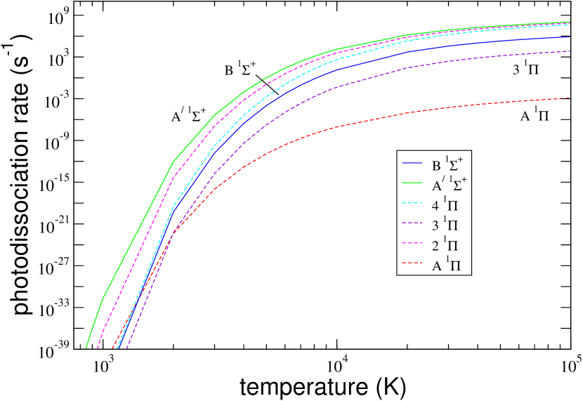
Figure 7: CS photorates in blackbody radiation fields for transitions from $v^{\prime\prime},J^{\prime\prime}=0,0$ to each excited electronic state as a function of radiation temperature.

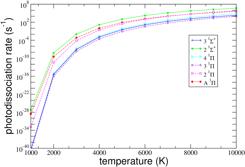
Figure 8: LTE blackbody photorates for each CS transition as a function of temperature when the kinetic and radiation temperatures are equal.

4 Conclusions

Accurate cross sections for the photodissociation of the CS molecule have been computed for transitions to several excited electronic states using new ab initio potentials and transition dipole moment functions. The state-resolved cross sections have been computed for nearly all rotational transitions from vibrational levels $v^{\prime\prime}=0$ through $v^{\prime\prime}=84$ of the $\text{X}\ ^{1}\Sigma^{+}$ ground electronic state of CS. Predissociation is found to be significantly smaller than direct photodissociation for CS. Additionally, LTE cross sections have been computed for temperatures ranging from 1000 to 10,000 K. The computed cross sections are applicable to the photodissociation of CS in a variety of UV-irradiated interstellar environments including diffuse and translucent clouds, circumstellar disks, and protoplanetary disks. Photodissociation rates in the interstellar medium and in regions with a blackbody radiation field have been computed as well. To facilitate the calculation of local photorates for particular astrophysical environments, all photodissociation cross section data can be obtained from the UGA Molecular Opacity Project website.

References

- Bergeman & Crossart (1981) Bergeman, T. & Crossart, D. 1981, JMoSp, 87, 119
- Bregman et al. (1978) Bregman, J. D., Goebel, J. H., & Strecker, D. W. 1978, ApJL, 223, L45
- Bruna et al. (1975) Bruna, P.J., Kammer, W.E., & Vasudevan, K. 1975, CP, 9, 91
- Cairnie et al. (2017) Cairnie, M., Forrey, R. C., Babb, J. F., Stancil, P. C., & McLaughlin, B. M. 2017, MNRAS, 471, 2481
- Canaves et al. (2007) Canaves, M., de Almeida, A., Boice, D., & Sanzovo, G. 2007, AdSpR, 39, 451
- Chang (1967) Chang, T. Y. 1967, RvMP, 39, 4
- Cooley (1961) Cooley, J. W. 1961, MaCom, 15, 363
- Coppens & Drowart (1995) Coppens, P. & Drowart, J. 1995, ChPhL, 243, 108
- Crawford & Shurcliff (1934) Crawford, F. H. & Shurcliff, W. A. 1934, Phys. Rev. A, 45, 860
- Destree, Snow, & Black (2009) Destree, J. D., Snow, T. P., & Black, J. H. 2009, ApJ, 693, 804
- Draine (1978) Draine, B. T. 1978, ApJS, 36, 595
- Draine & Lee (1984) Draine, B. T. & Lee, H. M. 1984, ApJ, 285, 89
- Edwards & Ziurys (2014) Edwards, J. L. & Ziurys, L. M. 2014, ApJ, 794, L27
- Forrey et al. (2016) Forrey, R. C., Babb, J. F., Stancil, P. C., & McLaughlin, B. M. 2016, JPhB, 49, 18
- Hasegawa et al. (1984) Hasegawa, T., Kaifu, N., Inatani, J., et al. 1984, ApJ, 283, 117
- Hayashi et al. (1985) Hayashi, M., Omodaka, T., Hasegawa, T., & Suzuki, S. 1985, ApJ, 288, 170
- Heays et al. (2017) Heays, A.N., Bosman, A.D., & van Dishoeck, E.F. 2017, A&A, 602, A105
- Helgaker et al. (2000) Helgaker, T., Jorgensen, P., & Olsen, J. 2000, Molecular Electronic-Structure Theory (New York: Wiley)
- Herpin et al. (2012) Herpin, F., Chavarría, L., van der Tak, F., et al. 2012, A&A, 542, A76
- Huber & Herzberg (1979) Huber, K. P., & Herzbeg, G. 1979, Molecular Spectra and Molecular Structure IV, Constants of Diatomic Molecules (New York, NY: Von Nostrand and Reinhold)
- Jackson et al. (1982) Jackson, M. W., Halpern, J. B., Feldman, P. D., & Rahe, J. 1982, A&A, 107, 385
- Johnson (1977) Johnson, B. R. 1977, JChPh, 67, 4086