Average performance analysis of the stochastic gradient method for online PCA

Abstract

This paper studies the complexity of the stochastic gradient algorithm for PCA when the data are observed in a streaming setting. We also propose an online approach for selecting the learning rate. Simulation experiments confirm the practical relevance of the plain stochastic gradient approach and that drastic improvements can be achieved by learning the learning rate.

1 Introduction

1.1 Background

Principal Component Analysis (PCA) is a paramount tool in an amazingly wide scope of applications. PCA belongs to the small list of algorithms which are extensively used in data science, medicine, finance, machine learning, etc. and the list is almost infinite. PCA is one of the basic blocks in the Geometric Science of Information. Computing singular/eigenvectors easily provides nonlinear embedding of data living on low dimensional manifold in a straightforward manner [2]. The other main geometric aspect of PCA lies in the fact that eigenvectors belong to the sphere and orthogonal families of eigenvectors belong to the Stiefel manifold, an information that we should take into account when computing these objects.

In the era of Big Data though, computing a set of singular vectors might turn to be a formidable task to achieve in practice since in many cases, one is not even able to store the data matrix itself in the RAM, not even mentioning running an algorithm on it. In the recent years, the need to handle massive datasets has revived a tremendous soaring of online techniques and algorithms which incorporate the data in an incremental fashion. Online convex optimisation is now a thriving field for dozens of important contributions a year, and a remarkable impact on the way statistical estimation and machine learning is undertaken in practice [5, 11, 8]. On the other hand, however, PCA lives in yet another realm, which cannot be directly reached using the techniques recently developed for convex optimisation. PCA can be performed using optimisation over the sphere and online versions of this nonconvex optimisation problem. Online or stochastic version of PCA have been extensively studied quite recently; see in particular the review [3] for a thorough analysis of the practical performance of online methods for PCA. On the theoretical side, [10, 9, 6, 1] propose very interesting results about the behavior of stochastic gradient type algorithms with different implementation details and under various assumptions. In particular, [9] provides a very elegant approach to the analysis of the stochastic projected gradient descent without any assumption on the spectral gap between the largest eigenvalue and the second largest eigenvalue.

1.2 Our contribution

The goal of the present paper is to study the online version of the stochastic gradient algorithm for PCA. In the setting we are interested in, the entries of the matrix we want to PCA are observed online, i.e. one empirical correlation coefficient at a time. Our two main contributions are the following.

• We extend the analysis presented in [9] to the online setting. In particular, we obtain a precise control on the average performance of the online method which does not depend on the separation between the first and the second eigenvalue.

• We provide a practical method to tune the learning rate, i.e. the stepsize of the gradient algorithm, based on a recent version proposed in [7] of the Hedge Algorithm [4].

1.3 Organisation of the paper

Our main results are presented in Section 2 where the algorithm is described and our main theorem is given. The proof of our main theorem is exposed in Section 3. Implementation and numerical experiments are given in Section 4. In particular, a simple method for choosing the learning rate is described in Section 4.1. The technical lemmæ which are used in the proof of Section 3 are gathered in Section 0.A at the end of the paper.

2 Main results

2.1 The stochastic projected gradient algorithm

Given a symmetric matrix $A\in\mathbb{R}^{d\times d}$, the projected gradient algorithm writes

$$w_{t+1} =(I+\eta A)w_{t}/\|(I+\eta A)w_{t}\|.$$ (1)

The stochastic gradient we will study in this paper is simply defined as

$$w_{t+1} =(I+\eta A_{t})w_{t}/\|(I+\eta A_{t})w_{t}\|$$ (2)

where $A_{t}$ is defined as

$$A_{t} =d^{2}\ A_{i_{t},j_{t}}\ e_{i_{t}}e_{j_{t}}^{*}$$ (3)

and $(i_{t},j_{t})$ is drawn uniformly at random from $\{1,\ldots,n\}^{2}$.

2.2 Main theorem

Theorem 2.1

Let $\varepsilon>0$ and assume that $\frac{1}{p}<\langle w_{0},v\rangle$ for a leading eigenvector $v$ of $A$. Define

$$V_{T} =w_{0}^{*}\ \prod_{i=T}^{1}(I+\eta A_{t})^{\ast}((1-\varepsilon)I-A)\prod_{t=1}^{T}(I+\eta A_{t})\ w_{0}.$$ (4)

Then for $T$ satisfying

$$T>\max\left(\frac{4p^{2}d^{2}}{\varepsilon},\frac{\log 4p\varepsilon^{-1}}{\log\left(1+\frac{\varepsilon}{pd^{2}}\right)}\right),$$ (5)

and $\eta=\frac{\varepsilon}{4pd^{2}}$, it holds that

$$\mathbb{E}[V_{T}]\leq-\frac{\varepsilon}{4p}(1+2\eta)^{T}.$$ (6)

Comparing our result with [9], we first note that the online setting does not satisfy the hypothesis for which the framework in [9] can be used. In fact, the matrices $A_{t}$ in the online setting are not positive semidefinite, otherwise the matrix $A$ would be a nonnegative matrix which is not the case. Regardless of this setback, [9] provides an upper bound for the expectation of $V_{T}$. In that case, [9] requires $T$ to be larger than $d^{4}p/\varepsilon^{2}*c^{2}$ for some large enough constant $c$. Therefore, in practice, we obtain a better lower bound.

3 Proof of the Theorem 2.1

In this section, we prove our main result, namely Theorem 2.1. Define

$$B_{T} =\prod_{t=T}^{1}(I+\eta A_{t})^{*}((1-\epsilon)I-A)\prod_{t=1}^{T}(I+\eta A_{t})$$ (7)

so that $V_{t}=w_{0}^{*}B_{T}w_{0}$. We have the following recurrence relation.

Lemma 1

We have that

$$\mathbb{E}[B_{T}] =\mathbb{E}[B_{T-1}]+\eta\left(A^{*}\mathbb{E}[B_{T-1}]+\mathbb{E}[B_{T-1}]A\right)$$

$$\hskip 28.45274pt+\eta^{2}d^{2}\mathrm{diag}\left(A^{*}\mathrm{diag}(\mathbb{E}[B_{T-1}])A\right).$$

Proof

Expand the recurrence relationship and take the expectation.

Expanding the recurrence in Lemma 1, we have

$$\mathbb{E}[V_{T}] \leq w_{0}^{\ast}(I+2\eta A)^{T}((1-\varepsilon)I-A)w_{0}$$

$$\quad+\eta^{2}d^{2}\sum_{i=1}^{T}\sum_{i=1}^{T}(1+2\eta)^{T-i}\|\mathrm{diag}(\mathbb{E}[B_{i-1}])\|\|w_{0}\|^{2}_{2}.$$ (9)

Using an eigendecomposition of $A$ and $\|w_{0}\|_{2}^{2}=1$ gives

$$\mathbb{E}[V_{T}] \leq\sum_{j=1}^{d}(1+2\eta s_{j})^{T}(1-\varepsilon-s_{j})w_{0,j}^{2}+\eta^{2}d^{2}\sum_{i=1}^{T}(1+2\eta)^{T-i}\|\mathrm{diag}(\mathbb{E}[B_{i-1}])\|.$$ (10)

where $s_{1}>\cdots>s_{d}$ denote the eigenvalue of $A$ and $w_{0,j}=\langle w_{0},v_{j}\rangle$ denotes the $j-th$ component of $w_{0}$ in the basis of the eigenvectors of $A$. Since $s_{1}=1$, this inequality rewrites

$$\mathbb{E}[V_{T}] \leq-\varepsilon(1+2\eta)^{T}w_{0,1}^{2}+\sum_{j=2}^{d}(1+2\eta s_{j})^{T}(1-\varepsilon-s_{j})w_{0,j}^{2}$$

$$+\eta^{2}d^{2}\sum_{i=1}^{T}(1+2\eta)^{T-i}\|\mathrm{diag}(\mathbb{E}[B_{i-1}])\|.$$ (11)

Lemma 7 gives

$$\mathbb{E}[V_{T}] \leq-\varepsilon(1+2\eta)^{T}w_{0,1}^{2}+(1+\frac{(1+2\eta(1-\varepsilon))^{T}}{\eta(T+1)})$$

$$+\eta^{2}d^{2}\sum_{i=1}^{T}(1+2\eta)^{T-i}\|\mathrm{diag}(\mathbb{E}[B_{i-1}])\|.$$ (12)

Factoring out $(1+2\eta)^{T}$, the inequality writes

$$\mathbb{E}[V_{T}] \leq(1+2\eta)^{T}\Big{(}-\varepsilon w_{0,1}^{2}+\frac{1}{(1+2\eta)^{T}}+\frac{(1+2\eta(1-\varepsilon))^{T}}{(1+2\eta)^{T}\eta(T+1)}$$

$$\quad\quad\quad+\eta^{2}d^{2}\sum_{i=1}^{T}(1+2\eta)^{-i}\|\mathrm{diag}(\mathbb{E}[B_{i-1}])\|\Big{)}$$ (13)

Lemma 6 implies that

$$\|\mathrm{diag}(\mathbb{E}[B_{k}])\| \leq 2\frac{\eta}{\eta d^{2}+1}\left(\frac{1}{1-\eta(\eta d^{2}+2)}-\frac{1}{1-\eta}\right)(1-\varepsilon)$$

$$+2\frac{\eta}{\eta d^{2}+1}\Big{(}\eta d^{2}\frac{1}{1-\eta(\eta d^{2}+2)}$$ (14)

$$\quad+\frac{1}{1-\eta}\Big{)}(2-\varepsilon)+\left(1+\frac{\eta^{2}d^{2}}{1-\eta(\eta d^{2}+2)}\right)(1-\varepsilon)$$

$$\leq 2\frac{\eta}{\eta d^{2}+1}\left(\frac{1-\varepsilon+(2-\varepsilon)\eta d^{2}}{1-\eta(\eta d^{2}+2)}+\frac{1}{1-\eta}\right)+\left(1+\frac{\eta^{2}d^{2}}{1-\eta(\eta d^{2}+2)}\right)(1-\varepsilon)$$

$$\leq 2\frac{\eta}{\eta d^{2}+1}\frac{2-\varepsilon+(2-\varepsilon)\eta d^{2}}{1-\eta(\eta d^{2}+2)}+1+\frac{\eta^{2}d^{2}}{1-\eta(\eta d^{2}+2)}$$ (15)

for all $k$. This simplifies into

$$\|\mathrm{diag}(\mathbb{E}[B_{k}])\| \leq 1+\frac{\eta^{2}d^{2}+4\eta}{1-\eta(\eta d^{2}+2)}.$$ (16)

Thus we obtain

$$\mathbb{E}[V_{T}] \leq(1+2\eta)^{T}\Big{(}-\varepsilon w_{0,1}^{2}+\frac{1}{(1+2\eta)^{T}}+\frac{(1+2\eta(1-\varepsilon))^{T}}{(1+2\eta)^{T}\eta(T+1)}$$

$$\hskip 14.22636pt+\eta^{2}d^{2}\left(1+\frac{\eta^{2}d^{2}+4\eta}{1-\eta(\eta d^{2}+2)}\right)\sum_{i=1}^{T}(1+2\eta)^{-i}\Big{)}$$ (17)

Bounding $\sum_{i=1}^{T}(1+2\eta)^{-i}$ by its infinite series $\sum_{i^{1}}^{\infty}(1+2\eta)^{-i}=(2\eta)^{-1}$ yields

$$\mathbb{E}[V_{T}] \leq(1+2\eta)^{T}\Big{(}-\varepsilon w_{0,1}^{2}+\frac{1}{(1+2\eta)^{T}}+\frac{(1+2\eta(1-\varepsilon))^{T}}{(1+2\eta)^{T}\eta(T+1)}$$ (18)

$$+\eta/2d^{2}\left(1+\frac{\eta^{2}d^{2}+4\eta}{1-\eta(\eta d^{2}+2)}\right)\Big{)}.$$ (19)

We can show that for well chosen $\eta$ and $T$, the term under parenthesis is less that $-\varepsilon/4p$. Taking for example $\eta=\frac{\varepsilon}{4Cpd^{2}}$ for some constant $C$ such that $\left(1+\frac{\eta^{2}d^{2}+4\eta}{1-\eta(\eta d^{2}+2)}\right)\leq 2$ and $T>\max(4p^{2}d^{2}C/\varepsilon,\log(4p\varepsilon^{-1})/\log(1+\varepsilon/(Cpd^{2})))$ gives the result. For a small enough $\varepsilon$, we can take $C=1$.

4 Implementation

4.1 Choosing the learning rate

In this section, we address the question of choosing the learning rate, i.e. the stepsize $\eta$ in iterations (2). Tuning the learning rate is essential in practice as it is well known to have a huge impact on the convergence speed of the method. Our idea to tune the learning rate is as follows:

• Choose the tolerance $\epsilon\in(0,1)$, and the algorithm’s parameters $R,\ K\in\mathbb{N}_{*}$, $\rho\in(0,1)$ and $\beta>0$.

• Burn-in period:

  • For $\eta\in\{\rho^{k}\}_{k=1:K}$, run $R$ gradient iterations in parallel whose iterates are denoted by $w_{t}^{(k,r)}$, $t=1,\ldots,B$.

  • Define $\pi^{(k)}_{0}=1/K$, $k=1,\ldots,K$. For $t=1,\ldots,B$, let

    $$L_{t}^{(k)} =\frac{2}{R(R-2)}\sum_{r<r^{\prime}=2,\ldots,R}\langle w_{t}^{(k,r)},w_{t}^{(k,r^{\prime})}\rangle,$$ (20)

    and for $k=1,\ldots,K$, define

    $$\pi_{t+1}^{(k)} =\pi_{t}^{(k)}\ \exp\left(\beta\ L_{t}^{(k)}\right).$$ (21)

  • Stop when $\max_{k=1,\ldots,K}\ L_{t}^{(k)}\geq 1-10\ \epsilon$.

• After burn-in:

  • Reset $R$ to 1 and $K$ to 1.

  • Normalise $\pi$.

  • At each step $t=B+1,\ldots$, choose the stepsize with probability $\pi_{B}$.

  • Stop when $L^{(1)}_{t}\geq 1-\epsilon$.

Choosing the parameter $\beta$ is more robust than choosing the learning rate. Moreover, a reasonably effective value for $\beta$ is given by (see [4]):

$$\beta =\sqrt{\frac{\log(K)}{B}}.$$ (22)

4.2 Numerical experiment

In this section, we present a simple numerical experiment which shows that

• The stochastic gradient method actually works in practice

• The adaptive selection of the learning rate/stepsize described in the previous subsection actually accelerates the method’s convergence drastically.

We run a simple experiment on a random i.i.d. Gaussian matrix of size $10000\times 10000$. The convergence of $(L^{(1)}_{t})_{t\in\mathbb{N}}$ to 1 of the plain stochastic gradient method is shown in Figure 1a below. The accelerated version’s convergence for the same experiment is shown in Figure 1b below. These results show that the method of the previous Section actually provides a substantial acceleration. We carefully checked that the selected learning rate is not equal to the smallest nor the largest value on the proposed grid of values between $2^{-3}$, $2^{-2}$, …$2^{17}$. The observed gain in convergence speed was by a factor of 8.75. Extensive numerical experiment demonstrating this behavior at larger scales will be included in an expanded version of this work.

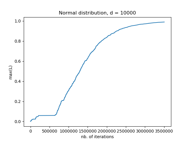
(a) $K=1$

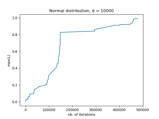
(b) $K=20$

Figure 1: Convergence of $(L^{(1)}_{t})_{t\in\mathbb{N}}$ as a function of the iteration index: (a) is for the case of the arbitraty choice of learning rate equal to $2^{-}4$ and (b) shows the behavior of the method using the learning procedure of Section 4.1 for values of the learning rate equal to $2^{-3}$, $2^{-2}$, $2^{-1}$, $1$, $2$, …, $2^{17}$.

Appendix 0.A Technical lemmæ

Recall that

$$B_{T} =\prod_{t=T}^{1}(I+\eta A_{t})^{*}((1-\varepsilon)I-A)\prod_{t=1}^{T}(I+\eta A_{t}).$$ (23)

Lemma 2

In the case of matrix completion, given a matrix $X$, we have

$$\mathbb{E}[A_{t}^{\ast}XA_{t}]=d^{2}\ \mathrm{diag}(A\ \mathrm{diag}(X)A).$$

Proof

The resulting matrix writes

$$A_{t}^{\ast}XA_{t} =d^{4}A_{ij}A_{ji}e_{j_{t}}e_{i_{t}}^{\ast}Xe_{i_{t}}e_{j_{t}}^{\ast}$$

$$=d^{4}A_{ij}A_{ji}X_{ii}e_{j_{t}}e_{j_{t}}^{\ast}.$$

Therefore the expected matrix writes

$$\mathbb{E}[A_{t}^{\ast}XA_{t}]=d^{2}\sum_{i,j}^{d}A_{ij}A_{ji}X_{ii}e_{j}e_{j}^{\ast}$$

Using the symmetry of $A$ gives the result.

Now our next goal is to see how $\mathrm{diag}\left(A^{*}\mathrm{diag}(\mathbb{E}[B_{T-1}])A\right)$ evolves with the iterations. For this purpose, take the diagonal of (LABEL:tototo), multiply from the left by $A^{*}$ and from the right by $A$ and take the diagonal of the resulting expression.

Recall that

$$\|A\|_{1\rightarrow 2} =\max_{j=1}^{d}\ \|A_{:,j}\|_{2}.$$

Lemma 3

We have that

$$\|\mathrm{diag}\left(\mathbb{E}[B_{T}]\right)\| \leq 2\eta\ \|\mathbb{E}[B_{T-1}]\|_{1\rightarrow 2}+(1+\eta^{2}d^{2})\ \|\mathrm{diag}(\mathbb{E}[B_{T-1}])\|$$ (24)

Proof

Expanding the recurrence relationship (LABEL:tototo) gives

$$\mathrm{diag}(\mathbb{E}[B_{T}]) =\mathrm{diag}(\mathbb{E}[B_{T-1}])+\eta\left(\mathrm{diag}\left(A^{*}\mathbb{E}[B_{T-1}]+\mathbb{E}[B_{T-1}]A\right)\right)$$

$$\hskip 28.45274pt+\eta^{2}d^{2}\mathrm{diag}\left(A^{*}\mathrm{diag}(\mathbb{E}[B_{T-1}])A\right).$$

For any diagonal matrix $\Delta$ and symmetric matrix $A$, we have

$$\|\mathrm{diag}(A^{\ast}\Delta A)\|\leq\|A\|_{1\rightarrow 2}^{2}\|\Delta\|.$$ (25)

Therefore, by taking the operator norm on both sides of the equality, we have

$$\|\mathrm{diag}(\mathbb{E}[B_{T}])\| \leq(1+\eta^{2}d^{2}\|A\|_{1\rightarrow 2}^{2})\|\mathrm{diag}(\mathbb{E}[B_{T-1}])\|+2\eta\|\mathrm{diag}(A^{*}\mathbb{E}[B_{T-1}])\|$$ (26)

We conclude using $\|\mathrm{diag}(A^{*}\mathbb{\mathbb{missing}}E[B_{T-1}])\|\leq\|A\|_{1\rightarrow 2}\|\mathbb{E}[B_{T-1}]\|_{1\rightarrow 2}$ and $\|A\|_{1\rightarrow 2}\leq 1$.

We also have to understand how the $\ell_{1\rightarrow 2}$ norm evolves.

Lemma 4

We have

$$\|\mathbb{E}[B_{T}]\|_{1\rightarrow 2} \leq\eta\ \|\mathbb{E}[B_{T-1}]\|+(1+\eta)\ \|\mathbb{E}[B_{T-1}]\|_{1\rightarrow 2}+\eta^{2}d^{2}\ \|\mathrm{diag}(\mathbb{E}[B_{T-1}])\|.$$ (27)

Proof

Expanding the recurrence relationship gives

$$\|\mathbb{E}[B_{T}]\|_{1\rightarrow 2} =\|\mathbb{E}[B_{T-1}]\|_{1\rightarrow 2}+\eta\ \left(\|A^{\ast}\mathbb{E}[B_{T-1}]\|_{1\rightarrow 2}+\|\mathbb{E}[B_{T-1}]^{\ast}A\|_{1\rightarrow 2}\right)$$

$$+\eta^{2}d^{2}\|\mathrm{diag}(A^{\ast}\mathrm{diag}(\mathbb{E}[B_{T-1}])A)\|_{1\rightarrow 2}.$$

For a diagonal matrix $\Delta$, we have $\|\Delta\|_{1\rightarrow 2}=\|\Delta\|$. This leads to

$$\|\mathbb{E}[B_{T}]\|_{1\rightarrow 2} =\|\mathbb{E}[B_{T-1}]\|_{1\rightarrow 2}+\eta\ \left(\|A\|\|E[B_{T-1}]\|_{1\rightarrow 2}+\|\mathbb{E}[B_{T-1}]\|\|A\|_{1\rightarrow 2}\right)$$

$$+\eta^{2}d^{2}\|A\|_{1\rightarrow 2}^{2}\|\mathrm{diag}(\mathbb{E}[B_{T-1}])\|.$$

Finally, using $\|A\|_{1\rightarrow 2}\leq 1$ concludes the proof.

We then have to understand how the operator norm of $\mathbb{E}[B_{T}]$ evolves

Lemma 5

We have

$$\|\mathbb{E}[B_{T}]\|\leq(1+2\eta)\|\mathbb{E}[B_{T-1}]\|+\eta^{2}d^{2}\ \|\mathrm{diag}(\mathbb{E}[B_{T-1}])\|.$$ (28)

Proof

Expanding the recurrence relationship (LABEL:tototo) return

$$\|\mathbb{E}[B_{T}]\|=\mathbb{E}[B_{T-1}]+\eta(\|A^{\ast}\mathbb{E}[B_{T-1}]\|+\|\mathbb{E}[B_{T-1}]A\|)+\eta^{2}d^{2}\|\mathrm{diag}(A^{\ast}\mathrm{diag}(\mathbb{E}[B_{T-1}])A)\|.$$

Then using similar inequalities as in the proof of the lemmas above, we have the result.

Lemma 6

Let $\|A\|=1$, then we have

$$\|\mathrm{diag}(A^{\ast}\mathrm{diag}(\mathbb{E}[B_{T}])A)\| \leq\alpha\max_{j}(1-\varepsilon-s_{j})+\beta\|(1-\varepsilon)I-A\|_{1\rightarrow 2}+\gamma\max_{j}(1-\varepsilon-A_{jj})$$ (29)

where

$$\alpha =2\frac{\eta}{\eta d^{2}+1}\left(\frac{1-\eta^{T-2}(\eta d^{2}+2)^{T-2}}{1-\eta(\eta d^{2}+2)}-\frac{1-\eta^{T-2}}{1-\eta}\right)$$

$$\beta =2\frac{\eta}{\eta d^{2}+1}\left(\eta d^{2}\frac{1-\eta^{T-2}(\eta d^{2}+2)^{T-2}}{1-\eta(\eta d^{2}+2)}+\frac{1-\eta^{T-2}}{1-\eta}\right)$$

$$\gamma =1+\eta^{2}d^{2}\frac{1-\eta^{T-2}(\eta d^{2}+2)^{T-2}}{1-\eta(\eta d^{2}+2)}$$

Proof

Expanding the recurrence and using equations (24), (27), and (28) yields the following system

$$\begin{bmatrix}\|\mathbb{E}[B_{T}]\|\\ \|\mathbb{E}[B_{T}]\|_{1\rightarrow 2}\\ \|\mathrm{diag}(\mathbb{E}[B_{T}])\|\end{bmatrix}\leq\left(I+\eta\begin{bmatrix}2&0&\eta d^{2}\\ 1&1&\eta d^{2}\\ 0&2&\eta d^{2}\end{bmatrix}\right)\begin{bmatrix}\|\mathbb{E}[B_{T-1}]\|\\ \|\mathbb{E}[B_{T-1}]\|_{1\rightarrow 2}\\ \|\mathrm{diag}(\mathbb{E}[B_{T-1}])\|\end{bmatrix}$$ (30)

To obtain the result, we expand the inequality by recurrence. Therefore, we are interested in computing the $T$-th power of the matrix in inequality (30). We have

$$\left(I+\eta\begin{bmatrix}2&0&\eta d^{2}\\ 1&1&\eta d^{2}\\ 0&2&\eta d^{2}\end{bmatrix}\right)^{T}=I+\sum_{i=1}^{T}\eta^{i}\begin{bmatrix}2&0&\eta d^{2}\\ 1&1&\eta d^{2}\\ 0&2&\eta d^{2}\end{bmatrix}^{i}.$$ (31)

After computing the power matrices, it result that

$$\|\mathrm{diag}(\mathbb{E}[B_{T}])\| \leq\sum_{i=1}^{T}\left(\eta^{i}\frac{2(\eta d^{2}+2)^{i-1}-1}{\eta d^{2}+1}\right)\|\mathbb{E}[B_{0}]\|$$

$$+\sum_{i=1}^{T}\left(\eta^{i}\frac{2\eta d^{2}(\eta d^{2}+2)^{i-1}+1}{\eta d^{2}+1}\right)\|\mathbb{E}[B_{0}]\|_{1\rightarrow 2}$$

$$+\left(1+\eta^{2}d^{2}\sum_{i=1}^{T}(\eta^{2}d^{2}+2\eta)^{i-1}\right)\|\mathrm{diag}(\mathbb{E}[B_{0}])\|.$$ (32)

We conclude after computing the sums and bounding from above $\|\mathbb{E}[B_{0}]\|$ by $\max_{j}(1-\varepsilon-s_{j})$.

Lemma 7

For $\eta<1$ and $\varepsilon>0$, we have

$$\max_{s\in[0,1]}(1+2\eta\ s)^{T}(1-\varepsilon-s)\leq 1+\frac{(1+2\eta(1-\varepsilon))^{T}}{\eta(T+1)}$$ (33)

Proof

Denote $f(s)=(1+2\eta\ s)^{T}(1-\varepsilon-s)$. Differentiating $f$ and setting to zero, we obtain

$$2\eta T(1+2\eta\ s)^{T-1}(1-\varepsilon-s)-(1+2\eta\ s)^{T}=0$$

$$\Longleftrightarrow 2\eta T(1-\varepsilon-s)-(1+2\eta\ s)=0$$

$$\Longleftrightarrow\frac{T(1-\varepsilon)-1/2\eta}{T+1}=s$$

Let $s_{c}=\frac{T-\varepsilon-1/2\eta}{T+1}$ denote this critical point. Consider the two following cases :

1. if $s_{c}\notin[0,1]$, then $f$ has no critical point in the domain and therefore is maximised at either domain endpoint, i.e.

   $$\max_{s\in[0,1]}f(s)=\max\{f(0)=1-\varepsilon,f(1)=-\varepsilon(1+2\eta)^{T}\}\leq 1$$

2. if $s_{c}\in[0,1]$, then $f$ is maximised at $s_{c}$ and the value of $f$ at $s_{c}$ is

   $$\Bigg{(}1+2\eta\frac{T(1-\varepsilon)-1/2\eta}{T+1}\Bigg{)}^{T}\Bigg{(}1-\varepsilon-\frac{T(1-\varepsilon)-1/2\eta}{T+1}\Bigg{)}$$

   $$=\Bigg{(}1+\frac{2\eta T(1-\varepsilon)-1}{T+1}\Bigg{)}^{T}\Bigg{(}\frac{1-\varepsilon+1/2\eta}{T+1}\Bigg{)}$$

   $$\leq(1+2\eta(1-\varepsilon))^{T}\Bigg{(}\frac{1+1/2\eta}{T+1}\Bigg{)}$$

   $$\leq\frac{(1+2\eta(1-\varepsilon))^{T}}{\eta(T+1)}.$$

Overall, the maximum value that $f$ can reach is less than $\max\{1,\frac{(1+2\eta(1-\varepsilon))^{T}}{\eta(T+1)}\}\leq 1+\frac{(1+2\eta(1-\varepsilon))^{T}}{\eta(T+1)}\}$. Hence the result.

References

• [1] Zeyuan Allen-Zhu and Yuanzhi Li, Lazysvd: Even faster svd decomposition yet without agonizing pain, Advances in Neural Information Processing Systems, 2016, pp. 974–982.
• [2] Afonso S Bandeira, Ten lectures and forty-two open problems in the mathematics of data science, 2015.
• [3] Hervé Cardot and David Degras, Online principal component analysis in high dimension: Which algorithm to choose?, arXiv preprint arXiv:1511.03688 (2015).
• [4] Yoav Freund and Robert E Schapire, A decision-theoretic generalization of on-line learning and an application to boosting, Journal of computer and system sciences 55 (1997), no. 1, 119–139.
• [5] Elad Hazan et al., Introduction to online convex optimization, Foundations and Trends® in Optimization 2 (2016), no. 3-4, 157–325.
• [6] Chi Jin, Sham M Kakade, Cameron Musco, Praneeth Netrapalli, and Aaron Sidford, Robust shift-and-invert preconditioning: Faster and more sample efficient algorithms for eigenvector computation, arXiv preprint arXiv:1510.08896 (2015).
• [7] Haipeng Luo and Robert E Schapire, Achieving all with no parameters: Adanormalhedge, Conference on Learning Theory, 2015, pp. 1286–1304.
• [8] Shai Shalev-Shwartz et al., Online learning and online convex optimization, Foundations and Trends® in Machine Learning 4 (2012), no. 2, 107–194.
• [9] Ohad Shamir, Convergence of stochastic gradient descent for pca, arXiv preprint arXiv:1509.09002 (2015).
• [10]  , A stochastic pca and svd algorithm with an exponential convergence rate., ICML, 2015, pp. 144–152.
• [11] Suvrit Sra, Sebastian Nowozin, and Stephen J Wright, Optimization for machine learning, Mit Press, 2012.