Constraints on the AGN flares as sources of ultra-high energy cosmic rays from the Fermi-LAT observations

Abstract

It is well known that if the most energetic cosmic rays ($E>10^{20}$ eV) were protons then their acceleration sites should possess some extreme properties, including gigantic luminosity. As no stationary sources with such properties are known in the local ($D<200$ Mpc) neighborhood of the Milky Way, it is highly likely that the UHECR acceleration takes place in some transient events. In this paper we investigate scenario where the UHECRs are produced in strong AGN flares. Using more than 7 years of the Fermi-LAT observations we select candidate flares and, using correlation between jet kinetic luminosity and its bolometric luminosity, estimate local kinetic emissivity of giant AGN flares: $\mathcal{L}\sim 3.7\times 10^{44}\mathrm{erg~{}Mpc^{-3}~{}{yr^{-1}}}$. This value is about an order of magnitude larger than the emissivity in the CRs with $E>10^{20}$ eV, thus making this scenario feasible, if the UHECR escape spectrum in these sources is rather hard and/or narrow. This shape of spectrum is predicted in a number of present models of strong relativistic collisionless shocks. Also the scenario of acceleration in AGN flares can accommodate constraints coming from the observed arrival distribution of UHECRs. Finally, we demonstrate that in case of heavier UHECR composition all the constraints are greatly relaxed.

1 Introduction

Despite huge efforts to identify sources of ultra-high energy cosmic rays (UHECR, $E>10^{18}~{}$eV), the problem of their origin is far from being resolved – we do not know where these particles are accelerated [1]. Pure common sense suggests that the acceleration to such extreme energies takes place in regions with some extreme conditions, and it can be demonstrated more rigorously using so-called “Hillas plot” [2]: acceleration of energetic particles requires non-trivial combination of source parameters, primarily magnetic field strength $B$ and acceleration region size $L$ and that severely decreases the number of potential sources (e.g., [3]). Active galactic nuclei (AGNs) are considered to be one of the most plausible candidates – it is very tempting to tap into a huge reservoir of energy coming from accretion of matter onto supermassive black hole. However, this model faces certain difficulties – a configuration needed for an effective acceleration is a very efficient photon source as well. It can be estimated that sources that can accelerate protons up to the highest energies exceeding $10^{20}$ eV will have a luminosity around $10^{47}~{}\mathrm{erg~{}s^{-1}}$ [4, 5, 6, 7]. On the other hand, production of observed UHECR is a local phenomenon, because due to an interaction with background photons the horizon of propagation of $10^{20}$ eV protons is smaller than 150 Mpc [8, 9]. The existence of Greisen-Zatsepin-Kuzmin (GZK) cut-off in the UHECR energy spectrum was discovered by the HiRes experiment [10] and lately confirmed with a very high statistical significance by the Pierre Auger and the Telescope Array observatories [11, 12]. The problem is rather self-evident — there are no steady sources with required luminosity in the local volume. It was suggested that this difficulty can be solved by dropping the ’steadiness’ condition – UHECRs can be accelerated in flares of AGNs. Flares with isotropic luminosity $>10^{50}~{}\mathrm{erg~{}s^{-1}}$ were observed [13], so it is theoretically possible to accelerate protons up to energies exceeding $10^{21}$ eV.

This model can be tested observationally. In order to do that we have used $\gamma$-ray observations of the Fermi-LAT in the high energy (HE, $E>100$ MeV) range. Fermi-LAT observes the whole sky every three hours since August 2008, providing almost uniform coverage with a high temporal resolution. We have focused on the ’local sources’ ($z<0.3$) because we wanted to avoid complications that arise due to a redshift evolution but still retain a decent statistics, with a probed volume that is 1000 times larger than a GZK volume.

We have selected all flares with a luminosity above the threshold corresponding to acceleration of UHECR protons to energies $E>10^{20}~{}$eV and calculated total fluence of these flares. That allowed us to obtain local emissivity in the HE $\gamma$-rays, estimate the kinetic emissivity, and finally obtain the ratio of UHECR to kinetic emissivity.

The paper is organized as follows: in Section 2 we describe the data and method of data analysis, Section 3 contains our results and discussion, and we draw conclusions in Section 4.

2 Data and method

The goal of the present work is to investigate whether AGNs can be possible sources of UHECRs with $E>10^{20}$ eV even in the case of the lightest (protonic) composition. Only sources with some extreme properties can accelerate protons to these energies [2, 3] and the closest stationary source of the kind resides far out the GZK volume $V_{\mathrm{GZK}}$, which we define as a sphere with a radius $R_{\mathrm{GZK}}=150~{}$Mpc – a mean attenuation free path of a particle with the initial energy of $10^{20}$ eV. However, strong flares of AGNs can possibly accelerate protons to the very highest energies [6, 7]. First, the threshold in luminosity which corresponds to the cosmic ray energy $E>10^{20}$ eV shall be defined. Let us consider a spherical blob within a jet. We assume that both particle acceleration and emission of the radiation take place in this blob. Let its radius and the magnetic field strength be $R^{\prime},B^{\prime}$ where the primes indicate the comoving reference frame. The stringent constraints on the size of the acceleration region and strength of the magnetic field [2] can be written out as follows:

$$B^{\prime}R^{\prime}\geq E^{\prime}/Ze,$$ (2.1)

where $E^{\prime}$ is the UHECR energy in the comoving frame, $Z$ is the charge of the particle (for the moment, we consider protons, but we keep $Z$ for generality). Next, let us connect the radiative luminosity $L_{\mathrm{r}}$ (by which we mean the synchrotron luminosity) to the energy of UHECR. Radiative luminosities in the observer’s and comoving frames are related as $L_{\mathrm{r}}=L^{\prime}_{\mathrm{r}}\Gamma^{4}$. If the radiation energy density in the blob is $U^{\prime}_{\mathrm{r}}$ then the flux from the unit surface area is $(c/4)U^{\prime}_{\mathrm{r}}$ and the luminosity of the spherical blob is $L^{\prime}_{\mathrm{r}}=\pi R^{\prime 2}cU^{\prime}_{\mathrm{r}}$, or, assuming energy equipartition between radiation and magnetic field, $L^{\prime}_{\mathrm{r}}=\pi R^{\prime 2}cU^{\prime}_{\mathrm{b}}=\pi R^{\prime 2}cB^{\prime 2}/8\pi\geq(c/8)(E^{\prime}/Ze)^{2}$. Since $E^{\prime}=E/\Gamma$, we finally obtain

$$L_{\mathrm{r}}\geq\frac{c}{8e^{2}}E^{2}\frac{\Gamma^{2}}{Z^{2}}\approx 4\times 10^{44}E_{20}\frac{\Gamma^{2}}{Z^{2}}\text{erg/s}$$ (2.2)

which is adopted in this paper as a threshold value; $E_{20}$ is the UHECR energy in units $10^{20}$ eV.

Equating magnetic and radiative energy densities is justified by the fact that the ratio of the luminosities at the two spectral peaks in SED is equal to the ratio of the synchrotron and magnetic energy densities (Eq. 5 of [14]) and typically, heights of two peaks in a BL Lac object’s SED are comparable (it will be seen later that our objects of interest are mostly BL Lacs). The same circumstance allows us to use $L_{\gamma}$, the high-energy luminosity in the range 0.1–100 GeV, as a reliable proxy of $L_{\mathrm{r}}$.

Once again, we try to link the maximal UHECR energy to an observable quantity through several steps: 1) get constraints on the magnetic field strength and the size of acceleration region via Hillas criterion, 2) link magnetic and radiative synchrotron energy densities on the basis of energy equipartition and observed SEDs, 3) finally, estimate the synchrotron luminosity from the gamma-ray luminosity using the properties of BL Lac SEDs. More discussion on these relations will be given in Section 3.4.

Note that in principle, energy gain can take place in so-called dark accelerators without considerable emission from leptons, but such models should realize very specific conditions, like linear accelerators in vicinity of rotating dormant black holes [17]. The magnetic field must be always parallel to the velocity of the leptons and this condition is not satisfied in usual stochastic Fermi acceleration taking place in the jets of the AGNs – one can not avoid abundant radiation from accelerated particles, especially leptons in this less ordered environments. Another possibility of ’dark acceleration’ arises in electron-starved environments: if $\epsilon_{e}$ was low then the radiation would be naturally suppressed. It is not easy to realize scenario of the kind in usual astrophysical conditions, particularly in ones existing in the AGN jets.

Flares satisfying the condition (2.2) have never been observed in $V_{\mathrm{GZK}}$. Nevertheless it is possible to calculate their local energetics using much larger test volume $V_{0}$: we have selected a sphere with a radius corresponding to $z=0.3,~{}V_{0}\sim 10^{3}V_{\mathrm{GZK}}$. This volume is large enough to avoid significant statistical fluctuations and still it is appropriate to neglect effects of cosmological evolution at $z<0.3$. We selected all flaring sources satisfying Eq. (2.2), that potentially could be the sites of UHECR acceleration.

For almost 10 years Fermi-LAT has been continuously observing the celestial sphere at energies $>100$ MeV. That allowed us to compile the full census of the very bright flares in the local Universe. We have made use of the second catalog of flaring gamma-ray sources (2FAV) based on Fermi All-Sky Variability Analysis (FAVA) [18]. This catalog is a collection of gamma-ray sources which show significantly higher (or lower) photon flux in a given time window as compared to what could be expected from the average flux from the source direction. The catalog is based on the Fermi observations during the first 7.4 years of the mission.

Among the AGNs in 2FAV we selected those within the test volume $V_{0}$. There are controversial determinations of $z$ for the source PMN J1802-3940: there are a number of works with lower estimation, $z=0.296$ while in several others the source is placed at much higher redshift, $z=1.32$. For the sake of robustness, we did not include the source in our analysis. Moreover, it is possible that some AGNs could be in high state for a time span longer than 7.4 years and therefore enter the catalog as steady sources. In order not to miss such objects, we checked 3FGL catalog for ’superluminous’ sources within $z=0.3$. For the sources with known redshift we approximated the isotropic equivalent radiative luminosity with $L_{\gamma}\sim 4\pi d^{2}F_{100}$, $d$ is the luminosity distance to the source assuming the standard cosmology ($H_{0}=69.6\text{km s}^{-1}\text{Mpc}^{-1},\Omega_{\mathrm{M}}=0.286$) and $F_{100}$ is the energy flux above 100 MeV taken from 3FGL. Only one source with the known $z\leq 0.3$, S5 0716+71, exceeded the threshold (2.2). This source is also in the 2FAV catalog and we included it in our analysis. The final list of selected AGNs consists of thirty eight sources and is shown in table 2.

Name	$z$	$l$	$b$	$E_{\mathrm{kin}}$	%	$L_{\mathrm{max}}$
PKS 0056-572	0.02	$300.9$	$-60.1$	0	0	0.0021
PKS 0131-522	0.02	$288.3$	$-63.9$	0	0	0.0084
Mkn 421	0.03	$179.8$	$65.0$	0	0	0.11
3C 120	0.03	$190.4$	$-27.4$	0	0	0.027
Mkn 501	0.03	$63.6$	$38.9$	0	0	0.037
1ES 1959+650	0.05	$98.0$	$17.7$	0	0	0.090
SBS 1646+499	0.05	$76.6$	$40.1$	0	0	0.035
3C 111	0.05	$161.7$	$-8.8$	0	0	0.052
AP Librae	0.05	$340.7$	$27.6$	0	0	0.059
5BZBJ1728+5013	0.06	$77.1$	$33.5$	0	0	0.058
PKS 0521-36	0.06	$240.6$	$-32.7$	0	0	0.16
1H 0323+342	0.06	$155.7$	$-18.8$	0	0	0.11
PKS 1441+25	0.06	$34.6$	$64.7$	0	0	0.36
BL Lacertae	0.07	$92.6$	$-10.4$	0	0	0.35
TXS 0518+211	0.11	$183.6$	$-8.7$	0	0	0.85
PKS 2155-304	0.12	$17.7$	$-52.2$	$6.1\times 10^{50}$	0.1	1.2
GB6 J1542+6129	0.12	$95.4$	$45.4$	0	0	0.27
1ES 1215+303	0.13	$188.9$	$82.1$	0	0	0.98
ON 246	0.14	$232.8$	$84.9$	$2.6\times 10^{51}$	0.4	1.5
PKS 1717+177	0.14	$39.5$	$28.1$	0	0	0.73
1ES 0806+524	0.14	$166.2$	$32.9$	0	0	0.50
OQ 530	0.15	$98.3$	$58.3$	0	0	0.45
3C 273	0.16	$290.0$	$64.4$	$6.8\times 10^{51}$	1.0	3.5
PKS 0829+046	0.17	$220.7$	$24.3$	$5.9\times 10^{50}$	0.1	1.1
PKS 0736+01	0.19	$217.0$	$11.4$	$9.2\times 10^{51}$	1.4	3.4
MG1 J021114+1051	0.20	$152.6$	$-47.4$	$2.0\times 10^{51}$	0.3	1.8
B2 2107+35A	0.20	$80.3$	$-8.4$	0	0	0.71
OX 169	0.21	$72.1$	$-26.1$	$3.1\times 10^{51}$	0.5	1.4
1H 1013+498	0.21	$165.5$	$52.7$	$5.3\times 10^{51}$	0.8	2.5
B2 2023+33	0.22	$73.1$	$-2.4$	$2.7\times 10^{53}$	41.4	4.0
PMN J0017-0512	0.23	$101.2$	$-66.6$	$7.4\times 10^{50}$	0.1	1.7
5BZQJ0422-0643	0.24	$200.8$	$-36.1$	0	0	0.91
PMN J1903-6749	0.26	$327.7$	$-26.1$	$2.0\times 10^{51}$	0.3	2.0
PKS 0301-243	0.26	$214.6$	$-60.2$	$1.7\times 10^{52}$	2.6	9.3
S2 0109+22	0.27	$129.1$	$-39.9$	$5.4\times 10^{52}$	8.2	3.7
GB6 J0937+5008	0.28	$167.4$	$46.7$	$6.1\times 10^{50}$	0.1	1.2
NVSS J223708-392137	0.30	$0.6$	$-59.6$	$3.3\times 10^{51}$	0.5	1.9
S5 0716+71	0.30	$144.0$	$28.0$	$2.8\times 10^{53}$	42.3	11

Table 1: The list of the analyzed AGNs. $z$, $l$, $b$ are the redshift and galactic longitude and latitude, $E_{\mathrm{kin}}$ is the kinetic energy produced in the flares in the source, % is the percentage of this energy in the total kinetic energy of all flares, $L_{\mathrm{max}}$ is the maximum isotropic equivalent radiative luminosity in the observation period, in units of ’critical luminosity’ $4\times 10^{46}\text{erg s}^{-1}$, assuming $\Gamma=10$. All the estimates were made with the aperture photometry method.

There are different ways to estimate the gamma flux with their own advantages and drawbacks. First, one can use aperture photometry (AP) light curves which are available, e.g., on the SSDC website. This simple approach does not distinguish between source and background photons, therefore the flux is inevitably overestimated, especially at low galactic latitudes. Second, one can obtain maximum likelihood (ML) flux estimates for each flare using a Fermi Science Tools routine gtlike. This approach is the most rigorous, but the total length of the time intervals to be analyzed and their number makes such a task more challenging. Therefore, we solve the task in two stages: first, calculate the kinetic energy output using AP data and estimate the contribution of each source; second, recalculate this quantity using ML, but only for the sources with large contribution.

At the first stage, we compute the flux from AP data obtained from SSDC and use it to find strong flares exceeding our threshold and after that estimate the total kinetic power in these flares. There are strong correlations between the flux in the high energy range, 0.1 – 100 GeV and both the radiative luminosity and kinetic luminosity of the jet. At the same time it is desirable to use observations at even higher energies ($>1$ GeV) in order to maximally avoid contamination by the background photons because the point-spread function of Fermi-LAT quickly deteriorates with decreasing energies. Our strategy is to calculate the AP flux in the range 1 – 100 GeV within 2 degrees from the source and extrapolate it down to 0.1 GeV in the assumption of a flat spectrum.

The threshold luminosity given by Eq. (2.2) depends on the bulk Lorentz factor of the jet. We used Lorentz factor $\Gamma=10$ as a robust benchmark value [19, 20, 21] and considered acceleration to energies higher than $10^{20}$ eV. These parameters set the threshold (2.2) at the level of $4\times 10^{46}$ erg/s. We have explicitly checked that the acceleration in this regime was not limited by the synchrotron losses. Due to a relatively long duration of flares ($>10^{5}~{}$s) constraints on the minimal size of the acceleration region are greatly relaxed, which in turn allows to decrease the magnitude of needed magnetic field and, therefore, importance of synchrotron losses, see e.g. eqs. (1) and (2) in [6]. After that we selected the time intervals where the estimated luminosity exceeds the threshold. In other words, we chose the time intervals when a given AGN can accelerate protons to energies higher than $10^{20}$ eV. As a proxy of the (synchrotron) radiative luminosity we use the energy flux in the range 0.1 – 100 GeV.

After that it was possible to estimate the total kinetic energy of these flares. One of the tightest correlation between the isotropic-equivalent gamma-ray luminosity $L_{\gamma}$ and the jet kinetic power $P_{\mathrm{jet}}$ was obtained in [22]:

$$\log P_{\mathrm{jet}}=A\log L_{\gamma}+B$$ (2.3)

where $A=0.51\pm 0.02$ and $B=21.2\pm 1.1$. We assume that, due to the beaming of the photons, we cannot observe all the blazars, but only a fraction of order $f_{b}\equiv\Omega_{b}/2\pi\sim 1/2\Gamma^{2}$ where $\Omega_{b}$ is the solid angle of each of the two jets. Therefore in order to obtain the estimate of the total kinetic energy within the test volume, for each source we integrate $P_{\mathrm{jet}}$ over the time intervals when the source is above the luminosity threshold, sum up the energies from all the sources and multiply the sum by $2\Gamma^{2}$. We stress that while $L_{\gamma}$ is the isotropic-equivalent luminosity, $P_{\mathrm{jet}}$ is not. $P_{\mathrm{jet}}$ is an estimation of the actual kinetic power of the jet. Division by $f_{b}$ in turn corrects the ’observed’ power for the sources with misaligned jets (which therefore are not observed as blazars). The kinetic energy outputs obtained for each source is shown in table 2. Their sum, after multiplication by $2\Gamma^{2}$, yields $(1.3\pm 0.2)\times 10^{56}$ erg. One can see that only a handful of the sources can potentially contribute to the acceleration of CRs of the highest energies. For these sources we constructed more accurate ML light curves with the 1 week cadence in the energy range 0.1–100 GeV with the Fermipy package [23] and used them instead of AP lightcurves. The refined kinetic energies are given in table 2. Note that the contribution from B2 2023+33 dropped down severely because of its low galactic latitude.

Table 2: Refined kinetic energies for the sources with the largest power contribution obtained using maximum likelihood approach. The column with the AP-calculated energies is repeated for reference.

The total kinetic energy which does not suffer from the drawbacks of AP any more is $\mathrm{(4.7\pm 1.0)}\times 10^{55}$ erg.

There is a caveat in using the empirical relation between $L_{\gamma}^{\mathrm{iso}}$ and $P_{\mathrm{jet}}$ from [22]: they estimated the kinetic power from the observations of the cavities around AGNs; these cavities were probably produced $10^{7}-10^{8}$ years ago and may not represent the current AGN power. However, the empirical relation between the luminosity and kinetic power is valid not only for AGNs, but also for GRBs, although in the latter case it should be used with some degree of caution, as it is still a matter of debate. Moreover, [24] traced the same relation down to the luminosities of X-ray binaries in the Milky Way during flares so that the whole relation spans over $\sim 17$ orders of magnitude in luminosity. This ’unified’ relation has the form $\log P_{\mathrm{jet}}=\alpha\log L+\beta$ where $L$ is the collimation corrected luminosity $L=f_{b}L_{\gamma}^{\mathrm{iso}}$, $\alpha=0.98\pm 0.02$ and $\beta=1.6\pm 0.9$. If we use this relation with the adopted value of $\Gamma=10$ instead of Eq. (2.3), the resulting kinetic energy is $(7.9\pm 1.6)\times 10^{55}$ erg. In the following, we use the former value of $\mathrm{4.7}\times 10^{55}$ erg.

The kinetic energy is divided by the timespan of observations (7.4 years) and by the volume $V_{0}$ – that gives the total kinetic emissivity. The value obtained is $3.7\times 10^{44}$ erg Mpc^-3 yr^-1. This should be compared with the emissivity in UHECRs. It was shown that the emissivity required to reproduce the UHECR data above $10^{18}$ eV should be of the order $10^{45}-10^{46}$ erg Mpc^-3 yr^-1 [25] which corresponds to $\sim 10^{43}-10^{44}$ erg Mpc^-3 yr^-1 above $10^{20}$ eV. Our own calculation which follows the approach of [26] using the photo-pion production cross-section from [27] and pair production cross sections from [28, 29] gave the values of $8.1\times 10^{43}$ erg Mpc^-3 yr^-1 and $1.4\times 10^{43}$ erg Mpc^-3 yr^-1 (see Appendix A). The first value corresponds to the UHECR intensity as observed by Telescope Array collaboration [12], and the second value corresponds to the intensity reported by the Pierre Auger collaboration [30]. Thus, the ratio of the UHECR emissivity to the AGNs’ jet kinetic power, according to our estimations, varies from $3.8\times 10^{-2}$ in case of the lower UHECR flux of Pierre Auger to $2.2\times 10^{-1}$ in case of the higher UHECR flux of Telescope Array. In Appendix C we show how this estimation is affected by the uncertainty of the threshold (2.2).

Let us outline once again the procedure we used to obtain the kinetic emissivity of blazars.

1. For each source, find the time intervals when the luminosity exceeds the threshold. We call such intervals ’flares’.

2. Within these intervals, convert the radiative luminosity to the kinetic power via Eq. (2.3) and integrate it over time to obtain the kinetic energy output from the source in flaring states over the whole timespan.

3. Sum up the energy outputs from all the sources and divide the sum by $f_{b}$, the beaming factor.

4. Divide by the volume and the timespan of the observations to obtain the average kinetic emissivity of flaring AGNs.

3 Discussion

3.1 UHECR isotropization and acceleration spectrum

In the previous section we have calculated emissivity in UHECRs $\mathcal{L}_{\mathrm{UHECR}}=8.1\times 10^{43}~{}\mathrm{erg~{}Mpc^{-3}~{}yr^{-1}}$ or $1.4\times 10^{43}$ erg Mpc^-3 yr^-1 from the observed flux (reported by Telescope Array or Pierre Auger) of these particles and compared it with the kinetic emissivity in the strong AGN flares which satisfy Eq. (2.2): $\mathcal{L}_{\mathrm{kin}}=3.7\times 10^{44}~{}\mathrm{erg~{}Mpc^{-3}~{}yr^{-1}}$. The latter one was calculated taking into account the fact that we can observe only a small fraction of all flaring sources and total observed kinetic emissivity should be multiplied by the number of unseen sources, $n=2\pi/\Omega_{b}\sim 2\Gamma^{2}$. The viability of the scenario crucially depends on the degree of UHECR beaming, $\Omega_{\mathrm{UHECR}}$. If the accelerated UHECRs remain strongly beamed with $\Omega_{\mathrm{UHECR}}\sim\Omega_{b}$, the UHECR emissivity $\mathcal{L}_{\mathrm{UHECR}}$ will be corrected for the beaming factor as well. As after this correction $\mathcal{L}_{\mathrm{UHECR}}$ will be much larger than $\mathcal{L}_{\mathrm{kin}}$ it would clearly make the model unfeasible.

The UHECRs can be effectively isotropised during their propagation towards the observer, increasing $\Omega_{\mathrm{UHECR}}$ up to value of order unity. The isotropization can take place either in the immediate vicinity of the flaring region, which in turn shall be very close to the AGN engine, or in the magnetized intracluster medium. Large values of $\Omega_{\mathrm{UHECR}}$ mean that the observed flux of cosmic rays is generated by large number of flares with only small fraction of them pointing at us. In [31, 32] it was shown that the average degree of isotropization should be high, otherwise we should have observed much stronger degree of anisotropy; only relative minority of sources could reside in void-like regions where somewhat lower degree of isotropization is expected.

Even then, the luminosity in the UHECRs with $E>10^{20}$ eV amounts to a sizable fraction of the full kinetic luminosity of suprathreshold AGN flares in the local Universe, $3.8\times 10^{-2}$ or $2.2\times 10^{-1}$ depending on the UHECR spectrum selected, either PA or TA. Nevertheless, from the point of view of pure energetics it is not impossible that these flares can be the primary sources of the CRs of the highest energies. More than that, relatively large value of the ratio of UHECR to the full kinetic luminosity allows to put stringent constraints on the properties of the spectrum of CRs produced in the flares. We demanded that the total amount of energy in these CRs could not exceed one half of the kinetic energy [33]. The spectrum of the UHECRs was described as a simple power-law, $\propto E^{-\alpha},~{}E_{\mathrm{min}}<E<E_{\mathrm{max}}=10^{21}~{}$eV bounded from above and below. The results in form of $E_{\mathrm{min}}(\alpha)$ curves are presented in the figure 1. We have also checked that the results are not considerably changed with an increased value of $E_{\mathrm{max}}=10^{22}$ eV. It can be seen that soft extended spectra are excluded with a high degree of confidence, and the spectrum of produced UHECR must be sufficiently hard and/or narrow. A lot of models predict the very same shape for the spectrum of particles escaping from relativistic collisionless shocks (e.g., [34, 35, 36]) or accelerated immediately in BH magnetospheres [37].

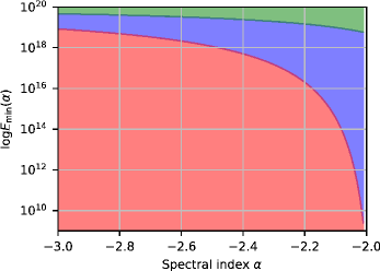
Figure 1: Constraints on the spectrum of the UHECRs produced in extreme AGN flares. The spectrum is described by a power law: $dN/dE\sim E^{\alpha},~{}E_{\mathrm{min}}(\alpha)<E<E_{\mathrm{max}}=10^{21}~{}$ eV. The green region allows to accommodate both TA and PAO data, the blue region is compatible to PAO data only and the red region is excluded.

Though we have used large test volume, very strong blazar flares necessary for acceleration of UHE protons are so rare, that still there is rather high level of statistical fluctuations in our estimations. If we took S5 0716+71 for an upward fluctuation and removed its contribution as an outlier then our estimations would drop by factor 6 that could pose severe problems for scenario in case of the TA spectrum. Low number of flare incidents in $V_{0}$ does not allow to evaluate distribution of flare properties.

Naturally, a large portion of lower energies UHECRs can also be accelerated in the AGNs. There are two factors that makes it more feasible: first, threshold luminosity becomes progressively lower ($L_{thr}\propto E^{-2}$), which in turn makes acceleration in less extreme flares or even steady sources possible. Second, at the same time, propagation distance quickly increases which enlarge the ’active volume’ and also enhance the observed flux. More detailed study of this scenario and its comparison with observed spectrum and, what is very important, mass composition at these energies will be done elsewhere.

3.2 Multimessenger considerations

Models with pure protonic composition can be constrained using secondary particles – cosmogenic neutrinos and gamma-rays which are generated in interactions of UHECRs with background (e.g. [38]). Cosmogenic photons via multiple $\gamma$-$e^{+}e^{-}$ conversions eventually cascade down to GeV-TeV energy range, and can contribute considerably to isotropic diffuse gamma-ray background at these energies. The latest results of the Fermi-LAT [39] have already allowed to strongly constrain protonic models at UHECR energies around $10^{18.2}$ eV [40]. On the other hand only models with a very strong redshift evolution are excluded at the highest energies [41]. The constraints from the cosmogenic neutrino are somewhat weaker but less model-dependent, they are still compatible with protonic models, again in the absence of strong evolution [42, 41]. It is worth noting that if UHECRs were accelerated in immediate vicinity of AGN engine, e.g. in inner jets, some fraction of high-energy neutrino could have been produced by UHECRs in photo-meson interactions, which in turn makes constraints coming from cosmogenic neutrinos more stringent [43]

3.3 UHECR source anisotropy

Small number of observed events with $E>10^{20}$ eV does not allow to perform meaningful large-scale anisotropy studies, it is still impossible to reliably distinguish between isotropic or some anisotropic distributions. Nevertheless, it is safe to claim that at any given moment the number of active sources in the $V_{\mathrm{GZK}}$ must be larger or equal than one [44]. We have observed $N=6$ potential sources in $t=7.4$ years inside $V_{0}=10^{3}~{}V_{\mathrm{GZK}}$ volume which gives the following estimate for the rate of extreme UHECR producing flares in the GZK volume:

$$\mathcal{R}\sim\frac{N}{t}\times\frac{V_{\mathrm{GZK}}}{V_{0}}\Gamma^{2}\sim 0.1~{}\mathrm{yr}^{-1}$$ (3.1)

Number of active UHECR sources can be readily estimated as

$$\mathcal{N}=\mathcal{R}t_{\mathrm{UHECR}},$$ (3.2)

where $t_{\mathrm{UHECR}}$ is the duration of observed UHECR signal. At first glance, given that the typical duration of gamma flares $t_{\gamma}$ are of order of weeks, this low rate seems to be at variance with the observations. However, being charged particles, UHECRs are subject to considerable deflection in the magnetic fields; when propagating short pulses are broadened by scattering:

$$\tau\sim d\theta_{s}^{2}/2c,$$ (3.3)

where $d$ is the propagation path length, $\theta_{s}$ is the characteristic angle of scattering. The observed duration $t_{\mathrm{UHECR}}=\tau$ can be much longer than $t_{\gamma}$. There are two closely related causes of scattering: first, there is a part due to the deflection in the random magnetic fields; second, there is considerable scattering due to a finite energy width of the pulse – cosmic rays at different energies are deflected by different angles.

There are several regions where scattering can possibly take place. At the very least, a pulse of UHECRs will be deflected in the Galactic magnetic fields. At these energies, the magnitude of scattering due to the random parts of the galactic magnetic field will be several tenth of degree for out of the Galactic plane directions [45], corresponding length is of order of kpc. Also the signal will be spread by several degrees in the regular galactic magnetic fields [46]. That translates to characteristic time scales $\tau$ around several decades. It could reach more than $10^{3}$ yr if a dipole field is present [47]. Also UHECRs will be scattered during inevitable isotropization in the vicinity of the source (see Section 3.1 above and [48, 49]) – the corresponding timescales are highly uncertain, they could be very large if the UHECRs were scattered in the magnetic fields of clusters, or, on the other hand, they could be insignificantly small if the primary site of the isotropization was very close to the source. Another sites of possible scattering include the local filament of the Large scale structure [50] or the extragalactic voids [51, 47]. In both cases deflections are expected to be lower than 10 degrees even in the most extreme scenarios. In the former case the characteristic length scale is $\mathcal{O}(Mpc)$ and the possible time delays could be of order $10^{5}$ years, when in the latter case they could exceed $10^{7}$ years. That means that at the highest energies we will simultaneously observe flares from at least $\mathcal{O}(10)$ sources and probably many more. It should be stressed that we do not demand isotropization of arrival directions of CRs coming from a single source because in case of light composition at these energies it would have required unreasonably high Galactic magnetic fields, like $\mathcal{O}(\mu G)$ strong magnetic field with a characteristic scale exceeding hundreds of kpc. Still, much smaller expected amplitudes of deflections and corresponding delays are sufficient to drastically increase number of simultaneously observed UHECR sources. Also a residual degree of anisotropy, like correlation with the local large scale structure is expected due to non-homogeinity of the matter distribution in the $V_{\mathrm{GZK}}$.

3.4 Blazar models

We should emphasize some underlying assumptions which are important to our approach, in particular to our using of Eq. (2.2). Namely, we assume that the synchrotron and magnetic field energy densities are approximately in equipartition. In the framework of SSC models, the ratio of these energy densities is equal to the ratio of the inverse Compton to synchrotron luminosity also known as Compton dominance. Although this parameter can vary in quite a wide range from one source to another, it is shown to increase systematically from BL Lacs to FSRQs, being around unity or even smaller for the former [52, 53]. In our Table 2, all the sources except 3C 273 and PKS 0736+01 are BL Lac objects. Moreover, the two most energetic sources in the list, S5 0716+71 and S2 0109+22 have been observed in a wide spectral range, in particular during a high state. Multiwavelength observations provide spectra of S5 0716+71 in the flaring state from which one can see that the inverse Compton peak is less significant than the synchrotron one [54]. The flaring spectrum of S2 0109+22 [55] shows two peaks of comparable magnitude. Similar picture is seen in other BL Lac blazars, e.g. Mkn 421, Mkn 501, 1ES 1959+650 [56, 57, 58]. If the high-energy peak of SED is lower than the synchrotron one, which is quite possible taking into account the observations cited, then using high-energy flux as a proxy, we underestimate the magnetic energy density and overestimate the threshold luminosity which makes the constraints on the UHECR acceleration spectrum more stringent. In this sense, our assumption of energy equipartition and the equality of the SED peaks is on the conservative side. Note that equipartition between electron and magnetic field energy is also considered to be likely the case. One argument is that the equipartition between electrons and magnetic field provides the minimal jet power compatible with the observed emission (see [59], chapter 5 for derivation and [60]). Equipartition is obtained as a result of numerical simulations of blazar jets. For example, [61] and [62] found rough equipartition between magnetic field and radiating particles in the reconnection model of blazar jets.

Our considerations refer to the one zone SSC model. In regard to BL Lacs, this is justified by observations. For example, [63] report on the significant correlation between optical and gamma variability of S5 0716+71 and [64] using a large sample of blazars found that optical and gamma-ray fluxes are correlated in BL Lacs (and in FSRQs, but to a lesser extent) which can be naturally explained in the SSC framework. On the other hand, there are plenty of sources where one zone SSC fails to fit all the data, e.g. for S5 0716+71. In this case more elaborated model is needed and, e.g., two zone SSC should be invoked instead. For our purposes we only need that the ratio of heights of the two spectral peaks still traces the ratio of magnetic and radiative energies. This is the case in the spine-layer model [15].

Apart from leptonic models, there is a whole class of hadronic and lepto-hadronic models [65] which can also be used to fit blazar SEDs, but result in different parameter values. However, within those models, it is difficult to relate the Poynting luminosity to some observed luminosity and the whole analysis deserves a separate investigation.

Some underestimation of real $\mathcal{L}_{\mathrm{kin}}$ can be due to a number of blazars without assigned redshift. There are 65 associated sources without assigned redshift in the 2FAV catalog, 57 of them would satisfy Eq. 2.2 if they were situated at $z=0.3$. In the highly unlikely scenario that all sources without estimated redshifts reside inside $V_{0}$ volume it will shift upwards our estimate of $\mathcal{L}_{\mathrm{kin}}$ by more than an order of magnitude and, accordingly, the estimate of energy available for UHECR acceleration, see Appendix C.

Finally, we have tried to evaluate how our results depended on the exact value of threshold (Eq. (2.2)) and repeated our calculations for two bracketing cases, i.e. $L_{\mathrm{r}}\geq 10^{46}~{}\mathrm{erg~{}s^{-1}}$ and $L_{\mathrm{r}}\geq 10^{47}~{}\mathrm{erg~{}s^{-1}}$, see Appendix C for details.

3.5 UHECR composition

We have chosen the lightest, protonic, composition for the UHECRs as a limiting scenario. From the theoretical point of view, acceleration of protons to the highest energies is very difficult, i.e. if it is possible for some class of sources to accelerate them, then, a fortiori, these sources can potentially produce UHECR nuclei with larger atomic number $A$. From the observational point of view, the composition of the UHECRs at the highest energies is still far from being certain: while the results of the Telescope Array experiment favor lighter one [66], the ones of Pierre Auger Observatory indicate that there is progressive increase in atomic number $A$ at higher energies [67]. However, due to a very low statistics there is no information about UHECR composition at the energies $E>10^{20}$ eV, so it is not inconceivable that we will eventually observe decrease in $A$. This issue will be hopefully resolved in the near future with analysis of the surface detectors data with their much larger duty cycle. First results of the TA collaboration analysis indicate presence of light UHECRs in the highest accessible energy bin ($\log E=19.6-20.0$) [69]. Also the latest results of the PAO SD show that the gradual increase in $A$ is apparently arrested at these energies [70].

On the other hand, the threshold luminosity given by the equation (2.2) is not known to the great accuracy, it can be several times higher or lower than the value we used (see Appendix C). This can strongly affect the conclusions we draw from our analysis in the assumption of protonic UHECR composition. Namely, if the threshold is significantly higher than that given by Eq. (2.2), then the kinetic emissivity of AGNs is insufficient to account for the observed UHECR intensity. Therefore it is reasonable to perform our analysis in the assumption of heavier composition. One can show that, in such case, the threshold luminosity used in our analysis lowers by $Z_{\mathrm{obs}}^{2}$, the charge of the observed nuclei squared. E.g. in the case of carbon nuclei, the threshold lowers by a factor of 36 to $10^{45}$ erg/s. In fact, at this level of gamma luminosity, we no longer need to seek for strong flares because there is quite a number of steady sources fulfilling the ’loosened’ criterion. Namely, we found 76 blazars in 3FGL with $z\leq 0.3$ and $L\geq 10^{45}$ erg/s. Their total kinetic emissivity appears to be $8\times 10^{45}~{}\mathrm{erg~{}Mpc^{-3}~{}yr^{-1}}$. The estimation of the theoretical UHECR emissivity depends on what nuclei are assumed to be accelerated at sources: the heavier the primaries, the lower emissivity is required to supply the observed intensity. The calculation is described in Appendix B. For the PAO data we obtained the emissivity of $3\times 10^{44}~{}\mathrm{erg~{}Mpc^{-3}~{}yr^{-1}}$ for carbon primaries and $5\times 10^{43}~{}\mathrm{erg~{}Mpc^{-3}~{}yr^{-1}}$ for silicon primaries. Our estimates show that, even for carbon, the ratio of UHECR emissivity to the total kinetic emissivity is less than 4% and is even lower for heavier primaries/observables. This makes the whole scenario more feasible. Also, due to stronger deflection of UHE nuclei in the magnetic fields and higher number of potential sources, the expected degree of anisotropy in this scenario is naturally lower.

4 Conclusions

The full census of strong local gamma-ray flares at redshifts $z<0.3$ from the Fermi-LAT data was used in order to find ones that can possibly accelerate protons to the highest energies $E>10^{20}$ eV and estimate maximal disposable amount of kinetic energy that can be potentially used for UHECRs acceleration. The estimated kinetic emissivity is approximately one order of magnitude higher than the UHECR emissivity obtained from the observations, that makes the scenario feasible from the point of view of total energetics, if the escape spectrum of cosmic rays is not too soft. Also, the number of potential sources in the Greisen-Zatsepin-Kuzmin volume is high enough, so no markedly anisotropic distribution of UHECRs is expected which is perfectly in line with the current observations. Thus, the giant flares of the AGNs similar to ones observed with the Fermi-LAT can be primary sources of the UHECRs with energies $E>10^{20}$ eV.

Appendix A UHECR emissivity: protons

Here we present the calculation of the UHECR emissivity in the local volume needed to provide the observed UHECR flux above $10^{20}$ eV. Let $N$ be the particle distribution function in space and energy and $E$ is the particle energy. In general, $N$ depends on the three space coordinates so that $\int N(\mathbf{r},E)dVdE$ is the number of the particles inside the volume $V$. Consider the propagation of the particles along coordinate $s$. The kinetic (transport) equation in one dimension is essentially the continuity equation in the space $(s,E)$ and can be written in the form

$$\frac{\partial N}{\partial t}=-\frac{\partial}{\partial s}(Nv)-\frac{\partial}{\partial E}\left(N\frac{dE}{dt}\right)+S$$ (A.1)

where $t$ is time, $v$ is the particle velocity, $dE/dt=vdE/ds$ is the energy loss rate, or the velocity in the energy space, and $S$ represents the source term. For our simple estimation we will assume that the medium is uniform and isotropic on the scale of 100 Mpc which justifies the use of one-dimensional approach and implies $\partial/\partial s\equiv 0$. We also assume stationarity on the scales of $\sim$300 Myr which leads to the relation $\partial/\partial t\equiv 0$. Moreover, at such relatively small scale we neglect the adiabatic losses. These assumptions leave us with

$$S=\frac{\partial}{\partial E}\left(Nv\frac{dE}{ds}\right).$$ (A.2)

The energy losses are due to photo-pion production and pair production, therefore

$$dE/ds=-E/\lambda_{\mathrm{attn}}$$ (A.3)

where $\lambda_{\mathrm{attn}}$ is the mean attenuation free path of a CR due to pion and pair production:

$$\frac{1}{\lambda_{\mathrm{attn}}}=\frac{1}{\lambda_{\mathrm{pion}}}+\frac{1}{\lambda_{\mathrm{pair}}}.$$ (A.4)

$\lambda_{\mathrm{pion}}$ can be obtained from eq. 10 of [26] via multiplication by the CR velocity $c$ and changing the order of integration:

$$\lambda_{\mathrm{pion}}=\frac{2\gamma^{2}\hbar^{3}\pi^{2}c^{3}}{kT}\times\left\{\int_{\epsilon_{\mathrm{th}}^{\prime}}^{\infty}d\epsilon^{\prime}\epsilon^{\prime}\sigma(\epsilon^{\prime})K_{p}(\epsilon^{\prime})[-\log(1-e^{-\epsilon^{\prime}/2\gamma kT})]\right\}^{-1}.$$ (A.5)

Here $T$ is the temperature of CMB, $\gamma$ is the Lorentz-factor of the UHECR, $\epsilon^{\prime}$ is the CMB photon energy in the UHECR rest frame, $\epsilon_{\mathrm{th}}^{\prime}$ is the pion production threshold energy, $\sigma(\epsilon^{\prime})$ is the photo-pion production cross-section and $K_{p}(\epsilon^{\prime})$ is the interaction inelasticity, or the mean fraction of the energy lost by an UHECR in a photo-pion production event. $\lambda_{\mathrm{pair}}$ can be found in [28]:

$$\lambda_{\mathrm{pair}}=\frac{\pi^{2}\hbar^{3}c^{3}}{\alpha r_{0}^{2}Z^{2}(mc^{2}kT)^{2}}\frac{E}{f(\nu)}$$ (A.6)

with $r_{0}$ the classical electron radius, $m$ the electron mass, $Z$ the UHECR charge, $\nu=mc^{2}/2\gamma kT$ and

$$f(\nu)=\nu^{2}\int_{2}^{\infty}d\xi\phi(\xi)(e^{\nu\xi}-1)^{-1}.$$ (A.7)

The approximation for the function $\phi(\xi)$ was taken from [29]. Equation (A.3) is equivalent to eq. 1 of [71].

For ultrarelativistic particles the density and intensity are related via

$$I=\frac{c}{4\pi}N,$$ (A.8)

hence, we obtain

$$S=-4\pi\frac{\partial}{\partial E}\frac{IE}{\lambda_{\mathrm{attn}}}$$ (A.9)

which in principle expresses the spectrum of the UHECR sources given the observed spectrum and the photo-pion production cross-section. Now the total energetic emissivity in UHECRs can be obtained via integration of the last equation over energies with the weight $E$:

$$\int_{E_{\mathrm{min}}}^{E_{\mathrm{max}}}ESdE=-4\pi\int_{E_{\mathrm{min}}}^{E_{\mathrm{max}}}E\frac{\partial}{\partial E}\frac{IE}{\lambda_{\mathrm{attn}}}dE=\left.\frac{4\pi E^{2}I}{\lambda_{\mathrm{attn}}}\right|^{E_{\mathrm{min}}}_{E_{\mathrm{max}}}+4\pi\int_{E_{\mathrm{min}}}^{E_{\mathrm{max}}}\frac{IE}{\lambda_{\mathrm{attn}}}dE$$ (A.10)

where $E_{\mathrm{min}}=10^{20}$ eV and $E_{\mathrm{max}}=10^{21}$ eV is the assumed upper energy limit of UHECR acceleration. The spectrum of cosmic rays above $10^{20}$ eV as observed by the Telescope Array collaboration can be represented in the form

$$I(E)=A\left(\frac{E\text{, eV}}{10^{20}}\right)^{-\gamma}$$ (A.11)

where $A=6.25\times 10^{-29}$ erg^-1cm^-2s^-1sr^-1 and $\gamma=4.6$ [12]. The spectrum in this energy range provided by the Pierre Auger collaboration reads

$$I(E)=I_{0}\left(\frac{E}{E_{a}}\right)^{-\gamma_{2}}\left[1+\left(\frac{E_{a}}{E_{s}}\right)^{\Delta\gamma}\right]\left[1+\left(\frac{E}{E_{s}}\right)^{\Delta\gamma}\right]^{-1}$$ (A.12)

where $I_{0}=3.30\times 10^{-19}$ eV^-1km^-2sr^-1yr^-1, $E_{\mathrm{a}}=4.8$ EeV, $E_{\mathrm{s}}=42$ EeV, $\gamma_{2}=2.60$ and $\Delta\gamma=3.14$ [30]. Substituting these expressions to (A.10) we obtain for TA and PA data $8.1\times 10^{43}$ and $1.4\times 10^{43}$ erg Mpc^-3yr^-1 respectively.

Appendix B UHECR emissivity: heavy nuclei

The calculation for heavy nuclei is different from that for protons due to the fact that they lose energy by photodisintegration which means they conserve the initial Lorentz factor while decreasing the energy. One can see from figure 2 of [72] that, in the energy range of interest ($>10^{20}$ eV) losses due to pair production are less than the photodisintegration losses. Only at about $A=40$ pair production starts to dominate at $\sim 10^{20}$ eV. We therefore neglected losses due to pair production. Then the transport equation for the nuclei of the sort $i$ is simply

$$\frac{\partial N_{i}(\Gamma)}{\partial t}=-\frac{N_{i}(\Gamma)}{\tau_{i}}+S_{i}(\Gamma)=0$$ (B.1)

where the term $N_{i}/\tau_{i}$ represents particle losses due to photodisintegration, $\tau_{i}$ being the mean time between disintegration events, and the term $S_{i}$ represents the sources. For the primary nuclei, the source term is a free parameter. For the rest of the nuclei the source term is equal to the loss term of the previous nucleus, i.e. $S_{i}=N_{i+1}/\tau_{i+1}$ so that the density of the nuclei of the mass $A$ can be obtained from the corresponding equation using the solution of the equation for the nuclei of the mass $A+1$. Under our assumptions, there is no loss term for protons. Moreover, for primary nuclei heavier than carbon accelerated to $10^{21}$ eV at maximum, protons can only have energies less than $10^{20}$ eV which is out of the range of interest of the present study. The primary source term assumed to obey the power law is adjusted so that the densities sum up to the observed quantity:

$$\sum_{i}N_{i}(E)=\frac{4\pi}{c}I(E)$$ (B.2)

We assumed acceleration in the energy range $10^{20}-10^{21}$ eV. Even for carbon, secondary protons appear to be outside this energy range and we did not take them into account. We used the data from PAO and obtained, for primary carbon, silicon and iron nuclei, the emissivities of $3\times 10^{44}$, $5\times 10^{43}$ and $4\times 10^{42}~{}\mathrm{erg~{}Mpc^{-3}~{}yr^{-1}}$ respectively, although the value for iron is underestimated due to the neglect of pair production.

Appendix C Uncertainty of threshold luminosity and unknown redshifts

The threshold (2.2) is not a well-defined quantity and its real value can deviate to a certain extent from the adopted value. We estimated the total kinetic luminosity as described in Section 2 with the threshold luminosities of $10^{46}$ erg/s and $10^{47}$ erg/s. The values obtained are $1.2\times 10^{45}$ erg Mpc^-3yr^-1 and $1.3\times 10^{44}$ erg Mpc^-3yr^-1. The latter value is rather close to the inferred UHECR emissivity which can make this scenario problematic.

Next, we note that in 2FAV catalog there are 65 sources with unknown redshifts. If we place them at the boundary of the test volume ($z=0.3$), then 57 of them exceed the threshold (2.2) at some times. Then we can calculate the ’hypothetical’ contribution of these sources to the overall kinetic luminosity. This contribution is equal to $7.1\times 10^{45}$ erg Mpc^-3yr^-1 (we excluded the sources within $5\mathrm{°}$ from the galactic plane). Obviously, this value makes the scenario more feasible, however we stress that we considered a highly unlikely case when all the sources with unknown $z$ reside at $z=0.3$ thus making the largest possible contribution to the total kinetic emissivity. Moreover, this calculation is made with aperture photometry and thus is an overestimation.

Finally we note that in the 3FGL catalog there are also a number of sources with unknown redshift. Analogously, we ’put’ them at the distance of $z=0.3$ and estimate their isotropic equivalent luminosity as $4\pi d^{2}F_{100}$ (see Section 2). We find that in such a case no source with unknown $z$ exceeds the threshold (2.2).

Acknowledgments

This work was supported by RSF research project No. 14-12-00146. The authors want to thank Andrei Gruzinov, Oleg Kalashev and Sergey Troitsky for fruitful discussions. The work was supported by the foundation for the Advancement of Theoretical Physics and Mathematics “Basis”. The authors acknowledge the support from the Program of development of M.V. Lomonosov Moscow State University (Leading Scientific School ’Physics of stars, relativistic objects and galaxies’). The analysis is based on data and software provided by the Fermi Science Support Center (FSSC). This research has made use of NASA’s Astrophysics Data System.

References

- [1] A. Letessier-Selvon and T. Stanev, Ultrahigh energy cosmic rays, Reviews of Modern Physics 83 (2011) 907 [1103.0031].
- [2] A. M. Hillas, The Origin of Ultra-High-Energy Cosmic Rays, ARA&A 22 (1984) 425.
- [3] K. V. Ptitsyna and S. V. Troitsky, PHYSICS OF OUR DAYS Physical conditions in potential accelerators of ultra-high-energy cosmic rays: updated Hillas plot and radiation-loss constraints, Physics Uspekhi 53 (2010) 691 [0808.0367].
- [4] R. V. E. Lovelace, Dynamo model of double radio sources, Nature 262 (1976) 649.
- [5] R. D. Blandford, Acceleration of Ultra High Energy Cosmic Rays, Physica Scripta Volume T 85 (2000) 191 [astro-ph/9906026].
- [6] G. R. Farrar and A. Gruzinov, Giant AGN Flares and Cosmic Ray Bursts, ApJ 693 (2009) 329 [0802.1074].
- [7] E. Waxman and A. Loeb, Constraints on the local sources of ultra high-energy cosmic rays, JCAP 8 (2009) 026 [0809.3788].
- [8] K. Greisen, End to the Cosmic-Ray Spectrum?, Physical Review Letters 16 (1966) 748.
- [9] G. T. Zatsepin and V. A. Kuz’min, Upper Limit of the Spectrum of Cosmic Rays, Soviet Journal of Experimental and Theoretical Physics Letters 4 (1966) 78.
- [10] HiRes collaboration, First observation of the Greisen-Zatsepin-Kuzmin suppression, Phys. Rev. Lett. 100 (2008) 101101 [astro-ph/0703099].
- [11] Pierre Auger collaboration, Observation of the suppression of the flux of cosmic rays above eV, Phys. Rev. Lett. 101 (2008) 061101 [0806.4302].
- [12] Telescope Array collaboration, The Cosmic Ray Energy Spectrum Observed with the Surface Detector of the Telescope Array Experiment, Astrophys. J. 768 (2013) L1 [1205.5067].
- [13] A. A. Abdo et al., Fermi Gamma-ray Space Telescope Observations of the Gamma-ray Outburst from 3C454.3 in November 2010, ApJ 733 (2011) L26 [1102.0277].
- [14] F. Tavecchio, L. Maraschi and G. Ghisellini, Constraints on the Physical Parameters of TeV Blazars, ApJ 509 (1998) 608 [astro-ph/9809051].
- [15] G. Ghisellini, F. Tavecchio and M. Chiaberge, Structured jets in TeV BL Lac objects and radiogalaxies. Implications for the observed properties, A&A 432 (2005) 401 [astro-ph/0406093].
- [16] Y. Inoue and Y. T. Tanaka, Baryon Loading Efficiency and Particle Acceleration Efficiency of Relativistic Jets: Cases for Low Luminosity BL Lacs, ApJ 828 (2016) 13 [1603.07623].
- [17] E. Boldt and P. Ghosh, Cosmic rays from remnants of quasars?, MNRAS 307 (1999) 491 [astro-ph/9902342].
- [18] S. Abdollahi, M. Ackermann, M. Ajello, A. Albert et al., The second catalog of flaring gamma-ray sources from the Fermi All-sky Variability Analysis, ArXiv e-prints (2016) [1612.03165].
- [19] G. Ghisellini and F. Tavecchio, Fermi/LAT broad emission line blazars, MNRAS 448 (2015) 1060 [1501.03504].
- [20] T. Savolainen, D. C. Homan, T. Hovatta, M. Kadler, Y. Y. Kovalev, M. L. Lister et al., Relativistic beaming and gamma-ray brightness of blazars, A&A 512 (2010) A24 [0911.4924].
- [21] O. Hervet, C. Boisson and H. Sol, An innovative blazar classification based on radio jet kinematics, A&A 592 (2016) A22 [1605.02272].
- [22] R. S. Nemmen, M. Georganopoulos, S. Guiriec, E. T. Meyer, N. Gehrels and R. M. Sambruna, A Universal Scaling for the Energetics of Relativistic Jets from Black Hole Systems, Science 338 (2012) 1445 [1212.3343].
- [23] M. Wood, R. Caputo, E. Charles, M. Di Mauro, J. Magill and Jeremy Perkins for the Fermi-LAT Collaboration, Fermipy: An open-source Python package for analysis of Fermi-LAT Data, ArXiv e-prints (2017) [1707.09551].
- [24] G. P. Lamb, S. Kobayashi and E. Pian, Extending the ‘energetic scaling of relativistic jets from black hole systems’ to include -ray-loud X-ray binaries, MNRAS 472 (2017) 475 [1705.09191].
- [25] R. Aloisio, P. Blasi, I. De Mitri and S. Petrera, Selected Topics in Cosmic Ray Physics, ArXiv e-prints (2017) [1707.06147].
- [26] F. W. Stecker, Effect of Photomeson Production by the Universal Radiation Field on High-Energy Cosmic Rays, Physical Review Letters 21 (1968) 1016.
- [27] Particle Data Group collaborationChin. Phys. C 40 (2016) 100001.
- [28] G. R. Blumenthal, Energy Loss of High-Energy Cosmic Rays in Pair-Producing Collisions with Ambient Photons, Phys. Rev. D 1 (1970) 1596.
- [29] M. J. Chodorowski, A. A. Zdziarski and M. Sikora, Reaction Rate and Energy-Loss Rate for Photopair Production by Relativistic Nuclei, ApJ 400 (1992) 181.
- [30] The Pierre Auger Collaboration, A. Aab, P. Abreu, M. Aglietta, E. J. Ahn, I. A. Samarai et al., The Pierre Auger Observatory: Contributions to the 34th International Cosmic Ray Conference (ICRC 2015), ArXiv e-prints (2015) [1509.03732].
- [31] K. Murase, C. D. Dermer, H. Takami and G. Migliori, Blazars as Ultra-high-energy Cosmic-ray Sources: Implications for TeV Gamma-Ray Observations, ApJ 749 (2012) 63 [1107.5576].
- [32] H. Takami, K. Murase and C. D. Dermer, Isotropy Constraints on Powerful Sources of Ultrahigh-energy Cosmic Rays at 1019 eV, ApJ 817 (2016) 59 [1412.4716].
- [33] E. G. Berezhko and D. C. Ellison, A Simple Model of Nonlinear Diffusive Shock Acceleration, ApJ 526 (1999) 385.
- [34] A. Meli and P. L. Biermann, Active galactic nuclei jets and multiple oblique shock acceleration: starved spectra, A&A 556 (2013) A88 [1207.4397].
- [35] N. Globus, D. Allard, R. Mochkovitch and E. Parizot, UHECR acceleration at GRB internal shocks, MNRAS 451 (2015) 751 [1409.1271].
- [36] A. M. Bykov, D. C. Ellison and S. M. Osipov, Nonlinear Monte Carlo model of superdiffusive shock acceleration with magnetic field amplification, Phys. Rev. E 95 (2017) 033207 [1703.01160].
- [37] K. Ptitsyna and A. Neronov, Particle acceleration in the vacuum gaps in black hole magnetospheres, A&A 593 (2016) A8 [1510.04023].
- [38] J. P. Rachen and P. L. Biermann, Extragalactic ultra-high energy cosmic rays. I. Contribution from hot spots in FR-II radio galaxies., A&A 272 (1993) 161 [astro-ph/9301010].
- [39] Fermi-LAT collaboration, The spectrum of isotropic diffuse gamma-ray emission between 100 MeV and 820 GeV, Astrophys. J. 799 (2015) 86 [1410.3696].
- [40] R.-Y. Liu, A. M. Taylor, X.-Y. Wang and F. A. Aharonian, Indication of a local fog of subankle ultrahigh energy cosmic rays, Phys. Rev. D 94 (2016) 043008 [1603.03223].
- [41] O. Kalashev, Constraining Dark Matter and Ultra-High Energy Cosmic Ray Sources with Fermi-LAT Diffuse Gamma Ray Background, in European Physical Journal Web of Conferences, vol. 125 of European Physical Journal Web of Conferences, p. 02012, Oct., 2016, 1608.07530, DOI.
- [42] J. Heinze, D. Boncioli, M. Bustamante and W. Winter, Cosmogenic Neutrinos Challenge the Cosmic-ray Proton Dip Model, ApJ 825 (2016) 122 [1512.05988].
- [43] K. Murase, Y. Inoue and C. D. Dermer, Diffuse neutrino intensity from the inner jets of active galactic nuclei: Impacts of external photon fields and the blazar sequence, Phys. Rev. D 90 (2014) 023007 [1403.4089].
- [44] S. V. Troitsky, Doublet of cosmic-ray events with primary energies eV, Soviet Journal of Experimental and Theoretical Physics Letters 96 (2012) 13 [1205.6435].
- [45] M. S. Pshirkov, P. G. Tinyakov and F. R. Urban, Mapping ultrahigh energy cosmic rays deflections through the turbulent galactic magnetic field with the latest rotation measure data, MNRAS 436 (2013) 2326 [1304.3217].
- [46] M. S. Pshirkov, P. G. Tinyakov, P. P. Kronberg and K. J. Newton-McGee, Deriving the Global Structure of the Galactic Magnetic Field from Faraday Rotation Measures of Extragalactic Sources, ApJ 738 (2011) 192 [1103.0814].
- [47] K. Murase and H. Takami, Implications of Ultra-High-Energy Cosmic Rays for Transient Sources in the Auger Era, ApJ 690 (2009) L14 [0810.1813].
- [48] S. Kalli, M. Lemoine and K. Kotera, Distortion of the ultrahigh energy cosmic ray flux from rare transient sources in inhomogeneous extragalactic magnetic fields, A&A 528 (2011) A109 [1101.3801].
- [49] H. Takami and K. Murase, The Role of Structured Magnetic Fields on Constraining Properties of Transient Sources of Ultra-high-energy Cosmic Rays, ApJ 748 (2012) 9 [1110.3245].
- [50] H. Yüksel, T. Stanev, M. D. Kistler and P. P. Kronberg, The Centaurus A Ultrahigh-energy Cosmic-Ray Excess and the Local Extragalactic Magnetic Field, ApJ 758 (2012) 16 [1203.3197].
- [51] M. S. Pshirkov, P. G. Tinyakov and F. R. Urban, New Limits on Extragalactic Magnetic Fields from Rotation Measures, Physical Review Letters 116 (2016) 191302 [1504.06546].
- [52] G. Fossati, L. Maraschi, A. Celotti, A. Comastri and G. Ghisellini, A unifying view of the spectral energy distributions of blazars, MNRAS 299 (1998) 433 [astro-ph/9804103].
- [53] J. D. Finke, Compton Dominance and the Blazar Sequence, ApJ 763 (2013) 134 [1212.0869].
- [54] MAGIC Collaboration, M. L. Ahnen et al., Multi-wavelength characterization of the blazar S5~0716+714 during an unprecedented outburst phase, ArXiv e-prints (2018) [1807.00413].
- [55] S. Ansoldi et al., The broad-band properties of the intermediate synchrotron peaked BL Lac S2 0109+22 from radio to VHE gamma-rays, MNRAS 480 (2018) 879 [1807.02095].
- [56] J. Aleksić, S. Ansoldi, L. A. Antonelli, P. Antoranz, A. Babic, P. Bangale et al., Unprecedented study of the broadband emission of Mrk 421 during flaring activity in March 2010, A&A 578 (2015) A22 [1412.3576].
- [57] M. L. Ahnen, S. Ansoldi, L. A. Antonelli, P. Antoranz, A. Babic, B. Banerjee et al., Multiband variability studies and novel broadband SED modeling of Mrk 501 in 2009, A&A 603 (2017) A31 [1612.09472].
- [58] N. Kaur, S. Chandra, K. S. Baliyan, Sameer and S. Ganesh, A Multiwavelength Study of Flaring Activity in the High-energy Peaked BL Lac Object 1ES 1959+650 During 2015-2016, ApJ 846 (2017) 158 [1706.04411].
- [59] J. J. Condon and S. M. Ransom, Essential Radio Astronomy. 2016.
- [60] C. D. Dermer, M. Cerruti, B. Lott, C. Boisson and A. Zech, Equipartition Gamma-Ray Blazars and the Location of the Gamma-Ray Emission Site in 3C 279, ApJ 782 (2014) 82 [1304.6680].
- [61] L. Sironi, M. Petropoulou and D. Giannios, Relativistic jets shine through shocks or magnetic reconnection?, MNRAS 450 (2015) 183 [1502.01021].
- [62] M. Petropoulou, L. Sironi, A. Spitkovsky and D. Giannios, Relativistic Magnetic Reconnection in Electron-Positron-Proton Plasmas: Implications for Jets of Active Galactic Nuclei, ApJ 880 (2019) 37 [1906.03297].
- [63] B. Rani et al., Radio to gamma-ray variability study of blazar S5 0716+714, Astron. Astrophys. 552 (2013) A11 [1301.7087].
- [64] T. Hovatta, V. Pavlidou, O. G. King, A. Mahabal, B. Sesar, R. Dancikova et al., Connection between optical and -ray variability in blazars, MNRAS 439 (2014) 690 [1401.0538].
- [65] M. Böttcher, A. Reimer, K. Sweeney and A. Prakash, Leptonic and Hadronic Modeling of Fermi-detected Blazars, ApJ 768 (2013) 54 [1304.0605].
- [66] Telescope Array collaboration, Study of Ultra-High Energy Cosmic Ray composition using Telescope Array’s Middle Drum detector and surface array in hybrid mode, Astropart. Phys. 64 (2015) 49 [1408.1726].
- [67] Pierre Auger Collaboration, Depth of Maximum of Air-Shower Profiles at the Pierre Auger Observatory: Composition Implications, ArXiv e-prints (2014) [1409.5083].
- [68] Telescope Array collaboration, The Energy Spectrum of Ultra-High-Energy Cosmic Rays Measured by the Telescope Array FADC Fluorescence Detectors in Monocular Mode, Astropart. Phys. 48 (2013) 16 [1305.6079].
- [69] Telescope Array Collaboration, R. U. Abbasi et al., Mass composition of ultra-high-energy cosmic rays with the Telescope Array Surface Detector Data, ArXiv e-prints (2018) [1808.03680].
- [70] The Pierre Auger Collaboration, A. Aab, P. Abreu, M. Aglietta, I. F. M. Albuquerque, I. Allekotte et al., The Pierre Auger Observatory: Contributions to the 35th International Cosmic Ray Conference (ICRC 2017), ArXiv e-prints (2017) [1708.06592].
- [71] V. Berezinsky, A. Gazizov and S. Grigorieva, On astrophysical solution to ultrahigh energy cosmic rays, Phys. Rev. D 74 (2006) 043005 [hep-ph/0204357].
- [72] R. Aloisio, V. Berezinsky and S. Grigorieva, Analytic calculations of the spectra of ultra-high energy cosmic ray nuclei. I. The case of CMB radiation, Astroparticle Physics 41 (2013) 73 [0802.4452].