Holiest Minimum-Cost Paths and Flows in Surface Graphs

Let $G$ be an edge-weighted directed graph with $n$ vertices embedded on an orientable surface of genus $g$. We describe a simple deterministic lexicographic perturbation scheme that guarantees uniqueness of minimum-cost flows and shortest paths in $G$. The perturbations take $O(gn)$ time to compute. We use our perturbation scheme in a black box manner to derive a deterministic $O(n\log\log n)$ time algorithm for minimum cut in directed edge-weighted planar graphs and a deterministic $O(g^{2}n\log n)$ time proprocessing scheme for the multiple-source shortest paths problem of computing a shortest path oracle for all vertices lying on a common face of a surface embedded graph. The latter result yields faster deterministic near-linear time algorithms for a variety of problems in constant genus surface embedded graphs.

Finally, we open the black box in order to generalize a recent linear-time algorithm for multiple-source shortest paths in unweighted undirected planar graphs to work in arbitrary orientable surfaces. Our algorithm runs in $O(g^{2}n\log g)$ time in this setting, and it can be used to give improved linear time algorithms for several problems in unweighted undirected surface embedded graphs of constant genus including the computation of minimum cuts, shortest topologically non-trivial cycles, and minimum homology bases.

1 Introduction

Many recent combinatorial optimization algorithms for directed surface embedded graphs rely on a common assumption: the shortest path between any pair of vertices is unique. The most commonly applied consequence of this assumption is that the shortest paths entering (or leaving) a common vertex do not cross one another. From this consequence, one can prove near-linear running time bounds for a variety of problems, including the computation of maximum flows [4, 26, 5, 24] and global minimum cuts [53] in directed planar (genus $0$) graphs as well as the computation of minimum cut oracles in planar and more general embedded graphs [6, 3] (see also Wulff-Nilsen [68]).

This assumption is also used in algorithms for the multiple-source shortest paths problem introduced for planar graphs by Klein [46]. In the multiple-source shortest paths problem, one is given a surface embedded graph $G=(V,E,F)$ of genus $g$ with vertices $V$, edges $E$, and faces $F$. The goal is to compute a representation of all shortest paths from vertices on a common face $r\in F$ to all other vertices in the graph. Assuming uniqueness of shortest paths, multiple-source shortest paths can be computed in only $O(gn\log n)$ time [46, 11]. Algorithms for this problem can be used to solve a variety of problems in planar and more general surface embedded graphs of constant genus in near-linear time. Such results include the computation of shortest cycles with non-trivial topology [11, 32, 30, 27, 34, 2], the computation of maximum flows and minimum cuts [30, 41, 5, 28, 14, 49, 16], the computation of exact and approximate distance oracles [10, 44, 54], and even the computation of single-source shortest paths [47, 55].

Enforcing uniqueness.

Unfortunately, it is often difficult to actually enforce the assumption that shortest paths are unique. One popular method is to add tiny random perturbations to the lengths of edges, and then apply a variant of the Isolation Lemma of Mulmuley et al. [56] to argue that shortest paths are unique with high probability. This method is used directly by Erickson [26], Mozes et al. [53], Cabello et al. [11], and the numerous papers that rely on the latter result.

As an alternative to using randomness, one can instead use a lexicographic perturbation scheme where one redefines edge lengths to be multidimensional vectors so that comparisons can be done lexicographically. One such scheme was proposed by Charnes [17] and Dantzig et al. [20], and variants of it have been used for computing minimum cut oracles in planar graphs [35, 68, 6]. In short, the scheme turns every edge length into an $n+1$-dimensional vector where $n$ is the number of edges in the graph. The first component of the vector is the true length of the edge, but then there is a single other component set to $1$ based purely on the edge for which we are reassigning the length. Naively implementing the scheme adds an $O(n)$ time overhead to all operations involving edge length. There are faster ways to use the scheme depending on the application one has in mind. In particular, Cabello et al. [11] implement the scheme with only a $\log n$ factor increase in the running time of their multiple-source shortest paths algorithm. However, these fast implementations require some fairly heavy machinery, and even implementing Dijkstra’s [22] algorithm for single-source shortest paths requires that same $\log n$ factor increase in the running time and the use of relatively complex dynamic tree data structures [62, 38, 63]; see Cabello et al. [11, Section 6.2].

Parametric shortest paths and the leafmost rule.

Several algorithms for multiple-source shortest paths in embedded graphs [46, 11, 24] and maximum flows in planar graphs [4, 26, 24] rely (at least by some interpretations) on the parametric shortest paths framework introduced by Karp and Orlin [43, 69]. In short, these algorithms redefine the length of a subset of edges to increase or decrease by an amount equal to some parameter $\lambda$. The algorithms then continuously increase $\lambda$ while maintaining a shortest path tree $T$. At certain values of $\lambda$, an edge will pivot into $T$ while another edge pivots out. Uniqueness of shortest paths guarantees the total number of pivots to be small for the algorithms mentioned above.

That said, one can sometimes avoid the need for unique shortest paths by utilizing properties of planar embeddings. Klein [46], Borradaile and Klein [4], and Eisenstat and Klein [24] all give efficient algorithms that successfully use the parametric shortest path framework without doing anything explicit to the edge lengths to guarantee unique shortest paths. In particular, Eisenstat and Klein [24] give linear-time maximum flow and multiple-source shortest paths algorithms that cannot take advantage of the perturbation schemes mentioned above, because they crucially rely on the edge capacities/lengths being small non-negative integers. (Weihe [66] also describes a linear-time maximum flow algorithm for unweighted undirected planar graphs, and Brandes and Wagner [8] give an algorithm for unweighted directed planar graphs.)

Instead of using perturbation schemes, these algorithms all take advantage of the leafmost rule for selecting edges to pivot into the shortest path tree $T$. The leafmost rule works as follows: The edges outside of $T$ form a spanning tree $C$ of the planar dual graph. Consider rooting $C$ at some dual vertex (primal face); the root we choose depends upon the particular algorithm we are attempting to implement. When $\lambda$ reaches a value that requires pivoting an edge into $T$ but there are multiple appropriate candidate edges to choose from, the leafmost rule dictates that we should always select the candidate edge lying closest to a leaf of $C$. As a result, these algorithms all maintain leftmost shortest path trees, assuming the initial shortest path tree was itself leftmost. We note the leafmost rule bears a strong resemblance to Cunningham’s [19] rule for maintaining a strongly feasible basis during network simplex.

Despite these successes, the leafmost rule and leftmost shortest path trees still do not present an ideal solution for algorithms requiring unique shortest paths. For one, these algorithms need to be designed with leftmost shortest path trees in mind. In contrast, random perturbations and lexicographic perturbation schemes can be implemented with only minor changes in how comparisons and basic arithmetic operations are performed. And perhaps more seriously, there is no obvious generalization of leftmost shortest path trees or the leafmost rule for pivots in surface embedded graphs of non-zero genus. In particular, the complement of a spanning tree is not itself a tree in this case. Certain algorithms such as the multiple-source shortest paths algorithm of Cabello et al. [11] appear to crucially rely on a guarantee that shortest paths really are unique.

1.1 Our Results

Let $G$ be a graph of size $n$ embedded in an orientable surface of genus $g$ with lengths on the edges. We present a deterministic lexicographic perturbation scheme that guarantees uniqueness of shortest paths despite using only $O(g+1)$-dimensional vectors for the perturbed edge lengths. The perturbation terms we use are all integers of absolute value $O(n)$, so our scheme can be employed in any combinatorial algorithm implemented in the word RAM model. Using our scheme increases the asymptotic running time of such algorithms by at most a factor of $g$.

As detailed in Section 3, the perturbation vectors can be computed in $O(gn)$ time using a simple algorithm. In short, we compute a $2g$-bit signature $[e]$ for each edge $e$ so that the sum of edge signatures along a cycle characterizes the homology class of that cycle with coefficients in $\mathbb{Z}$. A cycle’s homology class describes how it wraps around the holes on a surface. We also compute a single integer $z(e)$ for each edge $e$ so that given a cycle $\gamma$ bounding a subset of faces $F^{\prime}\subseteq F$, the absolute value of the sum of these integers along $\gamma$ is equal to the number of faces in $F^{\prime}$. This latter assignment of integers is inspired in part by results of Park and Philips [58] and Patel [59] on the minimum quotient and sparsest cut problems in planar graphs. Our perturbation vectors contain both $[e]$ and $z(e)$, and it is not difficult to show that every (simple) cycle in $G$ has non-zero cost according to our lexicographic perturbation scheme. Uniqueness of shortest paths follows as an easy consequence.

In fact, our scheme can be used to modify the costs of edges in the more general minimum-cost flow problem, guaranteeing that the minimum-cost flow itself is unique. It turns out that our scheme encourages the selection of leftmost shortest paths or minimum-cost flows in planar graphs, so we refer to the unique optimal solutions to these two problems as homologically lexicographic least leftmost minimum-cost paths and flows, or holiest paths and flows, for short.

After describing our perturbation scheme for computing holiest paths and flows, we turn to its applications. Using our scheme in a black box manner, we immediately derandomize the recent $O(n\log\log n)$ time minimum cut algorithm for directed planar graphs by Mozes et al. [53].

Our scheme can also be used in the multiple-source shortest paths algorithm of Cabello et al. [11] for arbitrary surface embedded graphs, bringing its total running time to $O(g^{2}n\log n)$. Compared to the deterministic perturbation scheme they consider, our alternative provides a factor $(\log n)/g$ improvement in running time, and the implementation is considerably simpler. In turn, we obtain the same $(\log n)/g$ factor improvement to the deterministic versions of nearly every algorithm that uses their data structure. Cabello et al. actually require a slightly stronger condition than mere uniqueness of shortest paths, but we are able to show our scheme guarantees the condition holds in Section 5. The exposition in that section also helps set us up for our remaining results.

It turns out that holiest paths and flows are not only leftmost objects of minimum-cost, but our perturbation scheme also forces the aforementioned parametric shortest path based algorithms to choose leafmost edges during pivots. See Section 6. Based on this observation, we generalize the linear-time multiple-source shortest paths algorithm of Eisentstat and Klein [24] for small integer edge lengths so that it works in surface embedded graphs of arbitrary genus. Our generalization runs in $O(g(gn\log g+L))$ time where $L$ is the sum of the integer edge lengths. Like Eisenstat and Klein, we must assume every edge has a reversal, essentially modeling unweighted undirected graphs in the case that edge lengths are all $1$.

The high level idea behind our algorithm is to generalize the leafmost rule using our new perturbation scheme. When we must pivot an edge into the holiest shortest path tree $T$, we partition the set of candidate edges into collections based on the homology class of their fundamental cycles with $T$. We pick a collection based on the homology signature portion of our scheme’s perturbation vectors, and then essentially apply the leafmost rule to edges within that collection to select the one that enters $T$. Finding the leafmost edge requires individually checking edges to see which ones can be pivoted into $T$. Fortunately, we can charge the time spent checking these edges to changes in the homotopy class of the holiest paths to these edges’ endpoints. We give our algorithm and analysis in Section 7.

Finally, using our linear-time algorithm for multiple-source shortest paths, we immediately obtain new linear time algorithms for a variety of problems in unweighted undirected surface embedded graphs, including the computation of $s,t$- and global minimum cuts, shortest cycles with non-trivial embeddings, and shortest homology bases. By combining known works, one can obtain linear time algorithms for each of these problems, assuming the genus is a constant. However, our new algorithms improve the running time for computing cuts from $g^{O(g)}n$ to $2^{O(g)}n$, and they improve the running time for the other problems from $2^{O(g)}n$ to $O(\operatorname{poly}(g)n)$. In particular, ours are the first algorithms for the latter problems that simultaneously have polynomial dependency on $g$ and linear dependency on $n$. We describe these applications in Section 8.

1.2 Additional Related Work

Although they may sometimes go by different names such as uppermost or rightmost, the idea of computing leftmost paths and flows in planar graphs appears as far back as the original maximum flow-minimum cut paper of Ford and Fulkerson [33]. Several researchers have designed efficient algorithms for specializations of the maximum flow problem in planar graphs using this idea [1, 40, 36, 60, 66, 67, 4]. There is a deep connection between flows in planar graphs and shortest paths in their duals (see, for example, Venkatesan [65]). As far as we are aware, though, Klein [46] was the first to apply the idea of directly computing        most shortest path trees.

Khuller, Naor, and Klein [45] observed that the set of integral circulations in a planar graph form a distributive lattice, and solutions to the minimum cost circulation problem form a sublattice. Indeed, a planar circulation is the boundary of a potential function (or $2$-chain) on the faces, and the meet and join can be defined by taking the component-wise max and min of the potential function, respectively. Many of the flow algorithms mentioned above actually find the top or bottom element in the (sub)lattice. Depending on which specifics one chooses, our lexicographic perturbation scheme simply enforces that one choose the minimum flow or circulation according to this sublattice. Matuschke and Peis [51] show that the left/right relation on $s,t$-paths in planar graphs also forms a lattice.

Bourke, Tewari, and Vinodchandran [7] observed that the reachability problem for planar directed graphs lies in unambiguous log-space (UL). A key aspect of their algorithm is computing a set of lengths for the edges of a grid graph so that shortest paths are unique. Their edge weighting scheme was later extended to arbitrary planar graphs by Tewari and Vinodchandran [64] and graphs embedded on constant genus surfaces by Datta et al. [21]. This latter result is similar to ours in that the length of each edge is the linear combination of $O(g)$ separate length functions including parts that encode the topology of paths and one part encoding face containment for topologically trivial cycles. However, our lexicographic perturbation scheme is arguably easier to implement than Datta et al.’s scheme in that they (and Tewari and Vinodchandran [64]) must compute a straight-line embedding of a subgraph of the input, while we work directly with the graph’s combinatorial embedding. Also, they use about twice as many length functions as we use vector components, and it is unclear if their scheme is as directly useful as ours for designing a linear time algorithm for multiple-source shortest paths in embedded graphs with small integer edge lengths.

2 Preliminaries

We begin with an introduction to surface embedded graphs. For more background we refer the reader to books and surveys [37, 57, 23, 70, 18, 52] related to the topic.

Surfaces.

A surface or $2$-manifold with boundary $\Sigma$ is a compact Hausdorff space where every point lies in an open neighborhood homeomorphic to either the Euclidean plane or the closed half plane. The points whose neighborhoods are homeomorphic to the closed half plane constitute the boundary of the surface. Every component of the boundary is homeomorphic to the unit circle. A cycle in the surface $\Sigma$ is a continuous function $\gamma:S^{1}\to\Sigma$ where $S^{1}$ is the unit circle. Cycle $\gamma$ is simple if $\gamma$ is injective. A path $P$ in the surface $\Sigma$ is a continuous function $P:[0,1]\to\Sigma$; again, $p$ is simple if it is injective. A loop is a path $P$ such that $P(0)=P(1)$; in other words, it is a cycle with a designated base point. The genus of the surface $\Sigma$, which we denote as $g$, is the maximum number of pairwise disjoint simple cycles $\gamma_{1},\dots,\gamma_{g}$ in $\Sigma$ such that $\Sigma\setminus(\gamma_{1}\cup\dots\cup\gamma_{g})$ is connected. Surface $\Sigma$ is non-orientable if any subset of $\Sigma$ is homeomorphic to the Möbius band. Otherwise, $\Sigma$ is orientable. Up to homeomorphism, a surface is characterized by its genus, the number of boundary components, and whether or not it is orientable. We directly work only with orientable surfaces in this paper.

Let $P_{1}$ and $P_{2}$ be two paths in $\Sigma$. Paths $P_{1}$ and $P_{2}$ cross if no continuous infinitesimal perturbation makes them disjoint. Otherwise, we call them non-crossing. They are homotopic if one can be continuously deformed into the other without changing their endpoints. More formally, there must exist a homotopy between them, defined as a continuous map $h:[0,1]\times[0,1]\to\Sigma$ such that $h(0,\cdot)=p$ and $h(1,\cdot)=q$. Homotopy defines an equivalence relation over the set of paths with any fixed pair of endpoints. A cycle is contractible if it is homotopic to a constant map, and a loop is contractible if it is homotopic to its base point. The concatenation of a path $P$ and loop $\gamma$ with common endpoint is homotopic to $P$ if and only if $\gamma$ is contractible.

Graph embeddings.

The surface embedding of an undirected graph $G$ with vertex set $V$ and edge set $E$ is a drawing of $G$ on a surface $\Sigma$ which maps vertices to distinct points on $\Sigma$ and edges to internally disjoint simple paths whose endpoints lie on their incident vertices’ points. A face of the embedding is a maximally connected subset of $\Sigma$ that does not intersect the image of $G$. An embedding is cellular if every face is homeomorphic to an open disc. In a cellular embedding, every boundary component is covered by the image of a cycle in $G$. Let $F$ be the set of faces of a cellular embedding, and let $b$ be the number of boundary components. By Euler’s formula, $|V|-|E|+|F|=2-2g-b$.

To more easily support directed graphs, we will assume $G$ is connected and that its embedding is given as a rotation system. These embeddings are sometimes referred to as combinatorial embeddings as well (see, for example, Eisenstat and Klein [24]). Let $\vec{E}$ denote a collection of “directed edges” we refer to as darts. Let $rev:\vec{E}\to\vec{E}$ be an involution on the darts we refer to as their reversals. Each edge $e$ is an orbit in the involution $\mathit{rev}$. We refer to one dart in $e$’s orbit as the canonical dart of $e$ and denote it by $\vec{e}$. In addition to $\mathit{rev}$, we have a permutation $\pi:\vec{E}\to\vec{E}$. Each orbit of $\pi$ gives the counterclockwise cyclic ordering of darts “directed into” a vertex $v$. We refer to $v$ as the head of the darts in $v$’s orbit. Vertex $v$ is the tail of these darts’ reversals. Orbits of the permutation $\mathit{rev}\circ\pi$ give the clockwise ordering of darts around each face of the embedding. We use the notation $G=(V,E,F)$ to denote a surface embedded graph $G$ with vertex set $V$, edge set $E$, and face set $F$. From here on, we refer to such triples simply as graphs. In this setting, we can actually define the genus $g$ of $G$ to be the solution to $|V|-|E|+|F|=2-2g$.

Given a graph $G=(V,E,F)$, we define the dual graph $G^{*}=(F,E,V)$. The given graph $G$ is sometimes called the primal graph. Graph $G^{*}$ contains a vertex for every face of $G$, an edge for every edge of $G$, and a vertex for every face of $G$. Two dual vertices are connected by a dual edge if and only if the corresponding primal faces are separated by the corresponding primal edge. In terms of combinatorial embeddings, the vertices of the dual graph are the orbits of the permutation $\mathit{rev}\circ\pi$; moreover, the orbits of $\mathit{rev}\circ\pi$ define the cyclic order of darts directed into each dual vertex. The drawing of dart $d$ in the dual graph goes left to right across the drawing of $d$ in the primal graph.

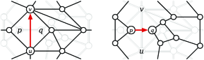
Figure 1: A dart $u\mathord{\shortrightarrow}v$ in the primal graph $G$ and the corresponding dart $p\mathord{\shortuparrow}q$ in the dual graph $G^{*}$.

For notational convenience, we will not distinguish between primal faces and dual vertices, primal and dual darts/edges, or dual vertices and primal faces. However, we will generally use the variables $u$, $v$, $w$, $x$, and $y$ to denote primal vertices/dual faces, and the variables $o$, $p$, $q$, and $r$ to denote dual vertices/primal faces. We let $u\mathord{\shortrightarrow}v$ denote a dart with tail $u$ and head $v$ in the primal graph, and let $p\mathord{\shortuparrow}q$ denote a dart with tail $p$ and head $q$ in the dual graph. Finally, $uv$ and $p\mathord{\mid}q$ denote edges between vertices $u$ and $v$ or between dual vertices $p$ and $q$, respectively. See Figure 1.

Flows, homology, and final definitions.

Flows are naturally defined either as non-negative functions on the darts (without loss of generality equal to zero on at least one dart of each edge) or as antisymmetric functions on the darts (where the values on the two darts of each edge sum to zero). It will prove convenient to use the non-negative formulation to describe flows in the primal graph $G$ and the antisymmetric formulation to describe flows in the dual graph $G^{*}$. For convenience in our proofs, our formal definitions will require non-negativity only when determining feasibility of flows.

A (primal) flow $f:\vec{E}\to\mathbb{R}$ is an assignment of real values to the darts of $G$. The imbalance $\delta{f}:V\to\mathbb{R}$ of flow $f$ is the net flow going into each vertex. Formally, $\delta{f}(v)=\sum_{u\mathord{\shortrightarrow}v}f(u\mathord{\shortrightarrow}v)-\sum_{v\mathord{\shortrightarrow}w}f(v\mathord{\shortrightarrow}w)$. Flow $f$ is a circulation if $\delta{(}v)=0$ for all $v\in V$. A potential function $\alpha:F\to\mathbb{R}$ is an assignment of real values to faces of $G$. We say flow $f$ is a boundary flow of potential function $\alpha$ if for every dart $u\mathord{\shortrightarrow}v=q\mathord{\shortuparrow}p$, we have $f(u\mathord{\shortrightarrow}v)-f(v\mathord{\shortrightarrow}u)=\alpha(p)-\alpha(q)$. In other words, high potentials to the right of darts encourage high flow values while high potentials to the left encourage low flow values. All boundary flows are circulations. Those familiar with concepts from algebraic topology may recognize the similarity between flows, imbalances, and potentials functions with $1$-chains, boundaries of $1$-chains, and $2$-chains, respectively. Two flows $f_{1}$ and $f_{2}$ are homologous if their componentwise difference is the boundary of some potential function. Similar to homotopy, homology defines an equivalence relation over any set of flows with identical vertex imbalances that is isomorphic with $\mathbb{R}^{2g}$.

A dual flow $z:\vec{E}\to\mathbb{R}$ assigns real values to the darts of the dual graph $G^{*}$ such that ${z(d)=-z(\mathit{rev}(d))}$ for every dart $d$. Equivalently, we consider a dual flow to be a function on the edges of $G^{*}$ by defining $z(e)=z(\vec{e})$. The dual imbalance $\partial{z}:F\to\mathbb{R}$ of dual flow $z$ is the total dual flow going clockwise around each primal face, or equivalently, into each dual vertex. Formally, $\partial{z}(p)=\sum_{q\mathord{\shortuparrow}p}z(q\mathord{\shortuparrow}p)$. Let $F^{\prime}\subseteq F$ be any subset of faces. Somewhat abusing notation, we let $\partial^{-}(F^{\prime})$ denote the clockwise neighborhood of $F^{\prime}$ so that $\partial^{-}(F^{\prime})=\{p\mathord{\shortuparrow}q:p\notin F^{\prime},q\in F^{\prime}\}$. Thus, darts of $\partial^{-}(F^{\prime})$ are directed clockwise around the boundary of $F\textquoteright$ in the primal graph $G$ and enter $F^{\prime}$ in the dual graph $G^{*}$.

Let $c:\vec{E}\to\mathbb{R}$ be a dart cost function, let $\mu:\vec{E}\to\mathbb{R}^{+}$ be a dart capacity function, and let $b:V\to\mathbb{R}$ be a vertex demand function. The cost of a flow $f$ is $c(f)=\sum_{d\in\vec{E}}f(d)\cdot c(d)$. A flow $f$ is feasible with respect to $\mu$ and $b$ if for all darts $d\in\vec{E}$ we have $0\leq f(d)\leq\mu(d)$ and for all vertices $v\in V$ we have $\delta{f}(v)=b(v)$. A minimum-cost flow with respect to $c$, $\mu$, and $b$ is a feasible flow of minimum cost (if it exists).

A (directed) path $P$ in $G$ is a sequence of darts $\langle v_{0}\mathord{\shortrightarrow}v_{1},v_{1}\mathord{\shortrightarrow}v_{2},\dots,v_{k-1}\mathord{\shortrightarrow}v_{k}\rangle$ where consecutive darts share vertices. We often abuse terminology and identify a path with its drawing in $G$’s embedding. A path is simple if it does not repeat any vertices, except possibly its first and last vertex. The concatenation of paths $P_{1}$ and $P_{2}$ is denoted $P_{1}\circ P_{2}$. Path $P$ is a cycle if $v_{0}=v_{k}$. Abusing notation, we may treat $P$ as a flow where $P(d)$ is equal to the number of times dart $d$ appears in $P$. Given a vertex $s\in V$, let $\mu:\vec{E}\to\mathbb{R}^{+}$ be a capacity function where $\mu(d)=\infty$ for all $d\in\vec{E}$, and let $b:V\to\mathbb{R}$ be a demand function where $b(v)=1$ for all $v\neq s$ and $b(s)=1-|V|$. Given dart costs $c:\vec{E}\to\mathbb{R}$ where no cycle has negative cost, the shortest paths from $s$ to all other vertices can be defined as the set of paths starting at $s$ and composing the minimum-cost flow with respect to $\mu$ and $b$. Let $\mathit{dist}_{c}(s,t)$ denote the distance from $s$ to $t$ according to costs $c$. Let $\sigma(s,t)$ denote the shortest path from $s$ to $t$.

A spanning tree $T$ of $G$ is a subset of edges that form a tree containing every vertex. We may root $T$ at a vertex $s$ by considering the darts of $T$ oriented away from $s$. Given a root $s$ and vertex $v\neq s$, the predecessor of $v$ in $T$ is the unique dart $u\mathord{\shortrightarrow}v$ that lies on the path from $s$ to $v$ in $T$. Given an edge $e\notin T$, the fundamental cycle of $e$ with $T$, denoted $\mathit{cycle}(T,e)$ is the unique simple cycle of edges in $T+e$. If $e\in T$, then $\mathit{cycle}(T,e)$ is empty. Given a dart $d$ of an edge $e$, its fundamental cycle $\mathit{cycle}(T,d)$ with $T$ is the orientation of $\mathit{cycle}(T,e)$ that contains $d$. A spanning cotree $C$ of $G$ is a subset of edges that form a spanning tree in the dual graph. We may root $C$ at a dual vertex $r$ by now considering the darts of $C$ oriented toward $r$. The successor of dual vertex $p\neq r$ is the dart $p\mathord{\shortuparrow}q$ that lies on the dual path from $p$ to $r$ in $C$. Dual vertex $o$ is a descendant of $p$ in $C$ if $p$ is on the dual path from $o$ to $r$ in $C$. A tree-cotree decomposition [25] of $G$ is a partition of $E$ into $3$ disjoint edge subsets $T,L,C$, where $T$ is a spanning tree of $G$, $C$ is a spanning cotree, and $L$ is a set of $2g$ leftover edges.

Given a vector $a$, let $a_{i}$ denote the $i$th component of $a$. Let $(T,L,C)$ be an arbitrary tree-cotree decomposition of $G$. Let $\Gamma=\langle\gamma_{1},\gamma_{2},\dots,\gamma_{2g}\rangle$ be some ordering of the $2g$ dual fundamental cycles of edges in $L$ with $C$, and orient each $\gamma_{i}$ in an arbitrary direction. The homology signature $[e]$ of an edge $e\in E$ with respect to $\Gamma$ is a $2g$-dimensional integer vector where $[e]_{i}=1$ if $\vec{e}\in\gamma_{i}$, $[e]_{i}=-1$ if $\mathit{rev}(\vec{e})\in\gamma_{i}$, and $[e]=0$ otherwise. We can compute homology signatures in $O(gn)$ time by computing $T$ and $C$ in $O(n)$ time and then taking an $O(n)$-time walk around each of the $O(g)$ cycles $\gamma_{i}$, updating the $i$th component of each edge’s signature vector along the walk. Given a dart $d$ of edge $e$, we define the homology signature of $d$ so that $[d]=[e]$ if $d=\vec{e}$ and $[d]=-[e]$ otherwise. Homology signatures given an implicit representation of a cohomology basis in $G$. See Erickson and Whittlesey [31] and subsequest papers [9, 30, 15, 2]. The homology signature of a flow $f$ is $[f]=\sum_{d\in\vec{E}}f(d)\cdot[d]$. Finally, we have the following lemma, easily derived by modifying known results for homology signatures.

Lemma 2.1

Let $f_{1}$ and $f_{2}$ be two flows. Flow $f_{i}$ is the boundary of some potential function if and only if $[f_{i}]=0$. Further, $f_{1}$ and $f_{2}$ are homologous if and only if $[f_{1}]=[f_{2}]$.

In particular, Lemma 2.1 implies that classes of flows with equivalent homology signatures do not depend upon the particular choice of basis used to define the signatures.

3 Holiest Perturbation

Let $G=(V,E,F)$ be a graph of size $n$ and genus $g$. Our lexicographic perturbation scheme relies on the properties of certain dual flows we refer to as drainages. Given a designated face $r\in G$, we define a drainage as a dual flow $z$ where $\partial{z}(q)<0$ for all $q\in F\setminus\{r\}$. The definition of a drainage immediately implies $\partial{z}(r)=-\sum_{q\in F\setminus\{r\}}\partial{z}(q)$. Because $r$ is the only face with positive dual imbalance with respect to $z$, we refer to $r$ as the sink of the drainage $z$.

We now describe our perturbation scheme. Let $c:\vec{E}\to\mathbb{R}$ be a dart cost function. We compute a set of homology signatures for the darts in $O(gn)$ time as described in Section 2. We then compute a drainage $z$ of $G^{*}$ in $O(n)$ time. While any drainage will do, we describe one here that is easily computed. We begin by computing an arbitrary spanning tree $C$ of $G^{*}$. Let $r\in F$ be an arbitrary face. We define $z$ as if each face $p\in F\setminus\{r\}$ is sending one unit of dual flow along $C$ to $r$.

Formally, we set the dual flow for each dart $p\mathord{\shortuparrow}q\in\vec{E}$ as follows. We root cotree $C$ at $r$. If $(p\mathord{\shortuparrow}q)$’s edge is not in $C$, then $z(p\mathord{\shortuparrow}q)=0$. Otherwise, if $p\mathord{\shortuparrow}q$ is the successor of $p$ in $C$, then $z(p\mathord{\shortuparrow}q)$ is the number of descendants of $p$ (including $p$ itself) in $C$; otherwise, $z(p\mathord{\shortuparrow}q)$ is the negation of the number of descendants of $q$ in $C$. One can easily verify that $\partial{z}(q)=-1$ for all $q\in F\setminus\{r\}$ and $\partial{z}(r)=|F|-1$.

We now redefine the costs of darts in $G$. Intuitively, we add a sequence of progressively smaller infinitesimal values to the cost of each dart based partially on the homology signatures of their edges and the dual flow they carry from the drainage $z$. More concretely, we define a new dart cost function $c^{\prime}:\vec{E}\to\mathbb{R}\times\mathbb{N}^{2g+2}$ as follows. Let ${+\!\!+}\,$ denote the concatenation of two vectors, and define

$$c\textquoteright(d):=(c(d),1){+\!\!+}\,[d]{+\!\!+}\,(z(d)).$$

The definition for the cost of a flow $f$ can be modified easily to work with our new cost function: $c^{\prime}(f)$ is the vector $\sum_{d\in\vec{E}}f(d)\cdot c\textquoteright(d)$. Given a cost vector $c^{\prime}$ for either a single dart or a whole flow, we refer to the components of dart and flow costs determined by homology signatures as the homology parts of $c^{\prime}$, denoted $[c^{\prime}]$. The last component is referred to as the face part and denoted $z(c^{\prime})$. Comparisons between dart and flow costs are performed lexicographically. As a consequence, any minimum-cost flow with respect to $c^{\prime}$ is also a minimum-cost flow with respect to the original scalar cost function $c$. Intuitively, minimizing the cost of a flow according to $c^{\prime}$ means first minimizing the original cost according to $c$, then minimizing the sum of the darts’ flow values, then lexicographically minimizing the homology class of the flow, and finally choosing the leftmost flow subject to all other conditions. In particular, when $g=0$, one is computing a leftmost minimum-cost flow (after also minimizing the sum of darts’ flows). The following lemma is immediate.

Lemma 3.1

For any flow $f$ and $j\in\{1,\ldots,2g\}$, we have $[f]_{j}=c^{\prime}_{j+2}(f)$. In addition,

$$c^{\prime}_{2g+3}(f)=\sum_{d\in\vec{E}}f(d)\cdot z(d).$$

Computing the perturbations takes $O(gn)$ time total. The time for every addition, multiplication, and comparison is now $O(g)$ instead of $O(1)$. For planar graphs in particular, this scheme requires only linear preprocesing time, and combinatorial algorithms relying on the new costs do not have higher asymptotic running times. Note that the cost of each dart $d$ is strictly larger than $(c(d),0,\ldots,0)$. No negative-cost directed cycles are created, even when some directed cycles had length $0$ originally, meaning shortest paths are still well-defined. In fact, the perturbation scheme does not create any new negative-cost darts, so combinatorial shortest path algorithms relying on non-negative dart costs still function correctly. As stated, however, these algorithms and those for negative costs do slow down by a factor of $g$.

3.1 Analysis

We now prove our perturbation scheme guarantees uniqueness of minimum-cost flows and shortest paths as promised. We begin by discussing the former as the latter follows as an easy consequence. The key observation behind our proof is that drainages encode the total imbalance of vertices lying on one side of a dual cut. In turn, we use this observation to show that every non-trivial circulation has a part of non-zero cost after using our perturbation scheme. The former observation is a slight generalization of one by Patel [59, Lemma 2.4] who in turn generalized a result for planar graphs by Park and Phillips [58]. We could use Patel’s result directly for the tree-based drainage described above. However, we are able to give a short proof of the more general lemma below.

Lemma 3.2

Let $z$ be a drainage with sink $r$, and let $F^{\prime}\subseteq F$. We have

$$\sum_{d\in\partial^{-}(F^{\prime})}z(d)=\sum_{q\in F^{\prime}}\partial{z}(q)=-\sum_{q\in F\setminus F^{\prime}}\partial{z}(q).$$

In particular, for non-empty $F^{\prime}\neq F$, we have $\sum_{d\in\partial^{-}(F^{\prime})}z(d)$ is positive if $r\in F^{\prime}$ and negative otherwise.

• We have

  $$\sum_{d\in\partial^{-}(F^{\prime})}z(d) =\sum_{p\mathord{\shortuparrow}q\in\vec{E}:p\notin F^{\prime},q\in F^{\prime}}z(p\mathord{\shortuparrow}q)+\sum_{p\mathord{\mid}q\in E:p,q\in F^{\prime}}[z(p\mathord{\mid}q)-z(p\mathord{\mid}q)]$$

  $$=\sum_{p\mathord{\shortuparrow}q\in\vec{E}:p\notin F^{\prime},q\in F^{\prime}}z(p\mathord{\shortuparrow}q)+\sum_{p\mathord{\mid}q\in E:p,q\in F^{\prime}}[z(p\mathord{\shortuparrow}q)+z(q\mathord{\shortuparrow}p)]$$

  $$=\sum_{p\mathord{\shortuparrow}q\in\vec{E}:q\in F^{\prime}}z(p\mathord{\shortuparrow}q)$$

  $$=\sum_{q\in F^{\prime}}\sum_{p\mathord{\shortuparrow}q\in\vec{E}}z(p\mathord{\shortuparrow}q)$$

  $$=\sum_{q\in F^{\prime}}\partial{z}(q).$$

  The final lemma statement follows easily from the definition of drainages.

Fix a cost function $c:\vec{E}\to\mathbb{R}$, and let $c^{\prime}$ be the perturbation of $c$ defined above. Also fix a capacity function $\mu:\vec{E}\to\mathbb{R}^{+}$ and a demand function $b:V\to\mathbb{R}$. We give the following lemma, which immediately implies the uniqueness of minimum-cost flows.

Lemma 3.3

Let $f_{1}$ and $f_{2}$ be distinct feasible flows with respect to $\mu$ and $b$. There exists a feasible flow $f$ such that at least one of $c^{\prime}(f)<c^{\prime}(f_{1})$ or $c^{\prime}(f)<c^{\prime}(f_{2})$ is true.

We emphasize that our perturbation scheme does not guarantee all feasible flows have distinct costs, and it may be that $c^{\prime}(f_{1})=c^{\prime}(f_{2})$. However, we would then have $f$ costing strictly less than both $f_{1}$ and $f_{2}$, implying neither $f_{1}$ nor $f_{2}$ is a minimum-cost feasible flow.

• We will prove existence of a circulation $\hat{f}$ such that $f_{i}+\hat{f}$ is feasible for some $i\in\{1,2\}$ and $c^{\prime}(\hat{f})<0$. We set $f=f_{i}+\hat{f}$, proving the lemma.

  Let $\tilde{f}=f_{2}-f_{1}$. Both $f_{2}$ and $f_{1}$ are feasible with respect to demand function $b$, so $\tilde{f}$ must be a non-trivial circulation. Further, for any dart $d$ and scalar $a$ with $0\leq a\leq 1$, we have

  $$f_{1}(d)+a\tilde{f}(d) =f_{1}(d)+a(f_{2}(d)-f_{1}(d))$$

  $$\geq\min\{f_{1}(d),f_{1}(d)+f_{2}(d)-f_{1}(d)\}$$

  $$\geq 0\text{ and}$$

  $$f_{1}(d)+a\tilde{f}(d) =f_{1}(d)+a(f_{2}(d)-f_{1}(d))$$

  $$\leq\max\{f_{1}(d),f_{1}(d)+f_{2}(d)-f_{1}(d)\}$$

  $$\leq\mu(d).$$

  In other words, we can add any circulation consisting of scaled down components of $\tilde{f}$ to $f_{1}$ and still have a feasible flow. Similarly, we can add any circulation consisting of scaled down components of $-\tilde{f}$ to $f_{2}$ and still have a feasible flow. We now consider two cases.

Case 1: $[\tilde{f}]\neq 0$.

Let $[\tilde{f}]_{j}$ be non-zero. Lemma 3.1 implies $c^{\prime}_{j+2}(\tilde{f})$ is also non-zero, further implying $c^{\prime}(\tilde{f})$ is itself non-zero. If $c^{\prime}(\tilde{f})<0$, then let $\hat{f}=\tilde{f}$. Otherwise, let $\hat{f}=-\tilde{f}$.

Case 2: $[\tilde{f}]=0$.

We consider two subcases.

First, suppose there exists an edge $e\in E$ such that $\tilde{f}(\vec{e})=\tilde{f}(\mathit{rev}(\vec{e}))>0$. Let $f_{e}:\vec{E}\to\mathbb{R}$ be a flow that is everywhere-zero except $f_{e}(\vec{e})=f_{e}(\mathit{rev}(\vec{e}))=\tilde{f}(\vec{e})$. Then, $c^{\prime}_{2}(f_{e})=2\tilde{f}(\vec{e})$, implying $c^{\prime}(f_{e})$ is non-zero. If $c^{\prime}(f_{e})<0$, then let $\hat{f}=f_{e}$. Otherwise, let $\hat{f}=-f_{e}$.

Now, suppose there is no such edge $e$ as defined above. Then, Lemma 2.1 implies $\tilde{f}$ is a boundary flow for some non-trivial potential function $\alpha$. Let ${\underline{\alpha}}=\min_{q\in F}\alpha(q)$ and ${\overline{\alpha}}=\max_{q\in F}\alpha(q)$. Because $\alpha$ is non-trivial, at least one of ${\underline{\alpha}}$ and ${\overline{\alpha}}$ is non-zero. Assume ${\overline{\alpha}}\neq 0$; the other case is similar. Let $F_{\overline{\alpha}}=\{q\in F:\alpha(q)={\overline{\alpha}}\}$, and let $\vec{E}_{\overline{\alpha}}=\{p\mathord{\shortuparrow}q\in\vec{E}:p\in F\setminus F_{\overline{\alpha}},q\in F_{\overline{\alpha}}\}$. For each dart $p\mathord{\shortuparrow}q\in\vec{E}_{\overline{\alpha}}$, we have $\tilde{f}(p\mathord{\shortuparrow}q)-\tilde{f}(q\mathord{\shortuparrow}p)>0$, because $\alpha(q)>\alpha(p)$.

Let $\varepsilon=\min_{d\in\vec{E}_{\overline{\alpha}}}(\tilde{f}(d)-\tilde{f}(\mathit{rev}(d)))$. For each dart $d\in\vec{E}_{\overline{\alpha}}$, let $a_{d}=\varepsilon/(\tilde{f}(d)-\tilde{f}(\mathit{rev}(d)))$. Note that $0<a_{d}\leq 1$. Finally, let $f_{\varepsilon}:\vec{E}\to\mathbb{R}$ be a flow that is everywhere-zero except for each dart $d\in E_{\overline{\alpha}}$, we have $f_{\varepsilon}(d)=a_{d}\tilde{f}(d)$ and $f_{\varepsilon}(\mathit{rev}(d))=a_{d}\tilde{f}(\mathit{rev}(d))$; in other words, $f_{\varepsilon}(d)-f_{\varepsilon}(\mathit{rev}(d))=\varepsilon$.

Let $z$ be the drainage used to define $c^{\prime}$. Lemmas 3.1 and 3.2 imply $c^{\prime}_{2g+3}(f_{\varepsilon})=\varepsilon\sum_{d\in\partial^{-}(F_{\overline{\alpha}})}$. Set $F_{\overline{\alpha}}$ is a non-empty strict subset of $F$, because $\tilde{f}$ is non-trivial. Therefore, Lemma 3.2 also implies $c^{\prime}_{2g+3}(f_{\varepsilon})$ is non-zero, meaning $c^{\prime}(f_{\varepsilon})$ is also non-zero. If $c^{\prime}(f_{\varepsilon})<0$, then let $\hat{f}=f_{\varepsilon}$. Otherwise, let $\hat{f}=-f_{\varepsilon}$.

Theorem 3.4

Let $G=(V,E,F)$ be a graph of genus $g$, let $c:\vec{E}\to\mathbb{R}$ be a dart cost function, and let $c^{\prime}:\vec{E}\to\mathbb{R}$ be the output of our lexicographic perturbation scheme on $c$. Let $\mu:\vec{E}\to\mathbb{R}^{+}$ and $b:V\to\mathbb{R}$ be a dart capacity and vertex demand function, respectively. The minimum-cost feasible flow with respect to $c^{\prime}$, $\mu$, and $b$ is unique and is a minimum-cost feasible flow with respect to $c$ as well.

Recall, the shortest $s,t$-path problem is a special case of minimum-cost flow where for each dart $d$, $\mu(d)=\infty$. In addition, all demands are zero except $b(t)=-b(s)=1$. Every directed cycle has its cost strictly increase, so if $c$ has no negative-length directed cycles, then $c^{\prime}$ has no negative or even zero-length directed cycles. Any feasible flow with a directed cycle $\gamma$ can be made cheaper by removing $\gamma$. The unique minimum-cost flow with respect to $c^{\prime}$ guaranteed by Theorem 3.4 is a directed path from $s$ to $t$.

Corollary 3.5

Let $G=(V,E,F)$ be a graph of genus $g$, let $c:\vec{E}\to\mathbb{R}$ be a dart cost function, and let $c^{\prime}:\vec{E}\to\mathbb{R}$ be the output of our lexicographic perturbation scheme on $c$. Let $s,t\in V$. The shortest $s,t$-path with respect to $c^{\prime}$ is unique and is a shortest $s,t$-path with respect to $c$ as well.

From here on, we refer to the unique minimum-cost flows and shortest paths guaranteed by our perturbation scheme as homologically lexicographic least leftmost or holiest flows and paths.

4 Minimum Cut in Directed Planar Graphs

As discussed in the introduction, our perturbation scheme can be used in a black box fashion to immediately derandomize the $O(n\log\log n)$ time minimum cut algorithm of Mozes et al. [53] for directed planar graphs. The only change necessary to derandomize their algorithm is to guarantee uniqueness of shortest paths in the dual graph.

Corollary 4.1

Let $G=(V,E,F)$ be a planar graph of size $n$, and let $c:\vec{E}\to\mathbb{R}$ be a dart cost function. There exists a deterministic algorithm that computes a global minimum cut of $G$ with respect to $c$ in $O(n\log\log n)$ time.

5 Multiple-Source Shortest Paths

Our scheme can be used in a black box fashion in the multiple-source shortest paths algorithm of Cabello et al. [11]. However, they depend on another property of the dart costs beyond uniqueness of shortest paths. Our perturbation scheme does guarantee the additional property, but we must first describe their algorithm in order to even explain what that property is. Understanding their algorithm is also a crucial first step in describing our linear-time algorithm for embedded graphs with constant genus and small integer dart costs. In order to more cleanly explain our linear-time algorithm in later sections, we describe a slight variant of Cabello et al.’s algorithm. This variant is based on the linear-time multiple-source shortest paths algorithm of Eisenstat and Klein [24] for planar graphs with small integer dart costs.

Let $G=(V,E,F)$ be an embedded graph of size $n$ and genus $g$, and let $c:\vec{E}\to\mathbb{R}$ be a cost function on the darts. Let $r\in F$ be an arbitrary face of $G$ from whose vertices we want to preprocess shortest paths with regard to $c$. The multiple-source shortest paths algorithm begins by computing a shortest path tree $T$ rooted at an arbitrary vertex of $r$. The algorithm proceeds by iteratively changing the source of the shortest path tree to each of the vertices in order around $r$; each change is implemented as a sequence of pivots wherein one dart $x\mathord{\shortrightarrow}y$ enters $T$ and another dart $w\mathord{\shortrightarrow}y$ leaves.

Consider one iteration of the algorithm where the source moves from a vertex $u$ to a vertex $v$. To move the source, the algorithm performs a special pivot. Let $x\mathord{\shortrightarrow}v$ be the predecessor dart of $v$ in $T$. During the special pivot, the algorithm removes dart $x\mathord{\shortrightarrow}v$ from $T$ and adds dart $v\mathord{\shortrightarrow}u$; afterward, $T$ is rooted at $v$. Let $\lambda\in\mathbb{R}$, and let $c_{\lambda}:\vec{E}\to\mathbb{R}$ be a parameterized cost function where $c(v\mathord{\shortrightarrow}u)=\lambda$ and $c_{\lambda}(d)=c(d)$ for all $d\neq v\mathord{\shortrightarrow}u$. This special pivot is accompanied by temporarily redefining the dart costs in terms of $c_{\lambda}$ with $\lambda$ initially set to $-\mathit{dist}_{c}(u,v)$. Changing the costs in this way guarantees that $T$ is a shortest path tree rooted at $v$ given dart $v\mathord{\shortrightarrow}u$ has cost $\lambda$.

Conceptually, the rest of the iteration is performed by continuously increasing $\lambda$ until it reaches $c(v\mathord{\shortrightarrow}u$), the original cost of $v\mathord{\shortrightarrow}u$, and maintaining $T$ as a shortest path tree as $\lambda$ is increased. Following convention from Cabello et al. [11], we say a vertex $x$ is red if the $v$ to $x$ path in $T$ uses dart $v\mathord{\shortrightarrow}u$; otherwise, the vertex is blue. Let $\mathit{dist}_{\lambda}$ denote $\mathit{dist}_{c_{\lambda}}$ for simplicity. Define the slack of dart $x\mathord{\shortrightarrow}y$ with regard to $\lambda$ to be

$$slack_{\lambda}(x\mathord{\shortrightarrow}y):=\mathit{dist}_{\lambda}(v,x)+c_{\lambda}(x\mathord{\shortrightarrow}y)-\mathit{dist}_{\lambda}(v,y).$$

For any $\lambda\in\mathbb{R},x\mathord{\shortrightarrow}y\in\vec{E}$, we have $slack_{\lambda}(x\mathord{\shortrightarrow}y)\geq 0$. We say dart $x\mathord{\shortrightarrow}y$ is tense if $slack_{\lambda}(x\mathord{\shortrightarrow}y)=0$. A spanning tree $T^{\prime}$ rooted at $v$ is a shortest path tree if and only if every dart in $T^{\prime}$ is tense. Dart $x\mathord{\shortrightarrow}y$ is active if $slack_{\lambda}(x\mathord{\shortrightarrow}y)$ is decreasing in $\lambda$. A dart $x\mathord{\shortrightarrow}y$ is active if and only if $x$ is blue and $y$ is red [11, Lemma 3.1]. All active darts see the same rate of slack decrease as $\lambda$ rises.

As $\lambda$ increases, it reaches certain critical values where an active dart $x\mathord{\shortrightarrow}y$ becomes tense. The algorithm then performs a pivot by inserting $x\mathord{\shortrightarrow}y$ into $T$ and removing the original predecessor $w\mathord{\shortrightarrow}y$ of $y$. Because $x\mathord{\shortrightarrow}y$ is tense when the pivot occurs, $T$ remains a shortest path tree rooted at $v$. Note that, with the exception of $v\mathord{\shortrightarrow}u$ during the special pivot, slacks do not change during pivots.

Using appropriate dynamic-tree data structures [61, 62, 38, 63], these critical values for $\lambda$ can be computed and pivots can be performed in amortized $O(\log n)$ time per pivot. Eisenstat and Klein use simpler data structures for the case of planar graphs with small integer costs; see Section 7 for details.

Across all iterations, the total number of pivots is $O(gn)$ [11, Lemma 4.3]. Therefore, between performing pivots and some $O(gn\log n)$ time additional work, the algorithm of Cabello et al. spends $O(gn\log n)$ time total. However, their algorithm and analysis depend upon two genericity assumptions: all vertex-to-vertex shortest paths are unique, and exactly one dart becomes tense at each critical value of $\lambda$.

Suppose we apply our lexicographic perturbation scheme so we are maintaining the holiest shortest path tree $T$. Let $c^{\prime}:\vec{E}\to\mathbb{R}\times\mathbb{N}^{2g+2}$ be the perturbed costs. Observe that $\lambda$ is now an increasing vector instead of a scalar. Corollary 3.5 guarantees that the first assumption is enforced. For the second assumption, we prove the following lemma.

Lemma 5.1

Consider an iteration where the source of $T$ moves from vertex $u$ to vertex $v$. For each value of $\lambda$, there is at most one active dart of minimum slack.

• Suppose there is at least one active dart. Let $\mu:\vec{E}\to\mathbb{R}^{+}$ be the dart capacities and $b:V\to\mathbb{R}$ be the vertex demands for shortest paths rooted at $v$, and let $f$ be the minimum-cost flow with respect to $c^{\prime}_{\lambda}$, $\mu$, and $b$ that uses darts of $T$. Let $b_{p}:V\to\mathbb{R}$ (‘p’ stands for pivot) be a vertex demand function that is zero-everywhere except $b_{p}(u)=-b_{p}(v)=1$, and let $c_{p}:\vec{E}\to\mathbb{R}^{+}$ be a residual cost function where $c_{p}(v\mathord{\shortrightarrow}u)=\infty$, $c_{p}(d)=-c^{\prime}_{\lambda}(\mathit{rev}(d))$ if $\mathit{rev}(d)\neq v\mathord{\shortrightarrow}u$ and $\mathit{rev}(d)$ lies on a shortest path according to $c^{\prime}_{\lambda}$, and $c_{p}(d)=c^{\prime}_{\lambda}(d)$ otherwise. Finding the active dart of minimum slack is equivalent to computing a holiest flow with respect to $c_{p}$, $\mu$, and $b_{p}$. However, the holiest flow is unique by Theorem 3.4.

After applying our perturbation scheme, the time to do basic operations on costs increases by a factor of $g$. In particular, we can construct the multiple-source shortest paths data structure of Cabello et al. [11] for unperturbed dart costs with only a $g$ factor increase in the construction time. The $O(gn\log n)$ space needed to store the final data structure is already more than the $O(gn)$ space we need to store perturbed edge lengths and auxiliary structures used during construction.

Theorem 5.2

Let $G=(V,E,F)$ be a graph of size $n$ and genus $g$, let $c:\vec{E}\to\mathbb{R}$ be a dart cost function, and let $r\in F$ be any face of $G$. We can deterministically preprocess $G$ in $O(g^{2}n\log n)$ time and $O(gn\log n)$ space so that the (unperturbed) length of the shortest path from any vertex incident to $r$ to any other vertex can be retrieved in $O(\log n)$ time.

6 The Leafmost Rule in Planar Graphs

In the previous section, we discussed using our perturbation scheme to efficiently solve the multiple-source shortest paths problem in embedded graphs. Recall, perturbations (deterministic or randomized) are not required for algorithms designed to compute multiple-source shortest paths exclusively in planar graphs [46, 24]. In fact, the linear-time algorithm of Eisenstat and Klein [24] cannot rely on perturbation schemes as it crucially depends upon all dart costs being small non-negative integers. Instead, these algorithms rely on the leafmost rule for selecting darts to pivot into the shortest path tree. The leafmost rule is also used in efficient $s,t$-maximum flow algorithms based on parametric shortest paths in the dual graph [4, 26, 24].

Let $G=(V,E,F)$ be a connected planar graph of size $n$, and let $c:\vec{E}\to\mathbb{R}$ be a cost function on the darts. Let $T$ be the shortest path tree maintained while running Section 5’s multiple-source shortest paths tree algorithm along face $r\in F$. Suppose we are moving the source of $T$ from vertex $u$ to vertex $v$, and let $v\mathord{\shortrightarrow}u=r\mathord{\shortuparrow}q$. Let $C$ be a spanning tree of $G^{*}$ complementary to $T$ with darts oriented toward $r$. In other words, the darts of $T$ and $C$ belong to distinct edges. The set of active darts are precisely the darts in the $q,r$-path through $C$ [11]. In this setting, the leafmost rule says we should pivot in the active dart of minimum slack that lies closest to a leaf of $C$; in other words, we choose the minimum slack dart encountered first on the $q$ to $r$ path through $C$. Following the leafmost rule guarantees we always maintain leftmost shortest path trees.

6.1 Modified Perturbation Scheme and the Leafmost Rule

We briefly return to the problem of computing multiple-source shortest paths around a face $r$ in a graph $G=(V,E,F)$ of arbitrary genus $g$. Consider the following slight modifications to our perturbation scheme described in Section 3. First, the drainage $z$ used to define the perturbed costs is required to use $r$ as its sink. We can easily compute such a drainage using a dual spanning tree as described in Section 3. Second, we forgo the $+1$ added as the second component to each dart’s cost, instead only using $2g+1$ integers based on the homology signatures and $z$ to perturb each dart’s cost. Let $c^{\prime}:\vec{E}\to\mathbb{R}\times\mathbb{N}^{2g+1}$ be the resulting perturbed costs.

The first modification described above has no effect on our scheme’s guarantee for minimum-cost flows and shortest paths. The second modification may have consequences, though. Namely, our modified scheme may introduce negative cost directed cycles where the original cost function had zero cost cycles, and minimum-cost flows and “shortest paths” may not be unique if a dart and its reversal both have zero cost. From this point forward, we will work under the assumption that every directed cycle has strictly positive cost according to the unperturbed cost function $c$.

Now, let us return to the planar setting for the rest of this section (so $g=0$). We claim the pivots chosen using the leafmost rule with dart costs $c$ are actually the same as the unique pivot choices guaranteed using perturbed costs $c^{\prime}$. We state this claim formally in the following lemma.

Lemma 6.1

Consider an iteration of the multiple-source shortest paths algorithm in planar graphs where the source of $T$ moves from vertex $u$ to vertex $v$. For each value of $\lambda$, the leafmost active dart of minimum slack according to $c$ is also the unique active dart of minimum slack according to $c^{\prime}$.

• We can assume the lemma holds inductively across earlier iterations of the algorithm and earlier values of $\lambda$ within the current iteration, meaning the current holiest path tree $T$ is the same for the algorithm using the leafmost rule with $c$ and the algorithm using perturbed costs $c^{\prime}$. Recall, the drainage $z$ used to define $c^{\prime}$ has sink $r$. Lemma 3.2 essentially states that the exact choice of $z$ does not matter; all drainages with equivalent dual imbalances result in the same unique minimum-cost flows and shortest paths in $G$. Therefore, we can assume without loss of generality that $z$ is non-zero only within the complementary dual spanning tree $C$ of $T$.

  Now, suppose there are two active darts $x\mathord{\shortrightarrow}y$ and $x^{\prime}\mathord{\shortrightarrow}y^{\prime}$ of minimum slack according to $c$. No darts along $\sigma(v,x)$, $\sigma(v,x^{\prime})$, $\sigma(u,y)$, or $\sigma(u,y^{\prime})$ have a non-zero face part to their perturbed costs. Therefore, $z(slack_{\lambda}(x\mathord{\shortrightarrow}y))=z(c^{\prime}(x\mathord{\shortrightarrow}y)-\lambda)$, and $z(slack_{\lambda}(x^{\prime}\mathord{\shortrightarrow}y^{\prime}))=z(c^{\prime}(x^{\prime}\mathord{\shortrightarrow}y^{\prime})-\lambda)$. That perturbation term is lower for whichever dart of $x\mathord{\shortrightarrow}y$ and $x^{\prime}\mathord{\shortrightarrow}y^{\prime}$ lies closer to the leaf of $C$.

The intuition provided by Lemma 6.1 will prove crucial in the next section where we describe our linear-time multiple-source shortest paths algorithm for small integer costs in embedded graphs of constant genus. While there does not appear to be an intuitive definition of leafmost in higher genus embedded graphs, we do have an equivalent perturbation scheme already defined for that setting. Our goal will be to efficiently find the unique pivots guaranteed by our use of the scheme.

Remark

We briefly remark that our perturbation scheme also explains the use of the leafmost rule in efficient $s,t$-maximum flow algorithms based on parametric shortest paths in the dual graph [4, 26, 24]. For this problem, the drainage is actually computed in the primal graph using $t$ as the sink.

7 Linear-time Multiple-Source Shortest Paths for Small Integer Costs

Let $G=(V,E,F)$ be an embedded graph of size $n$ and constant genus $g$ and let $r\in F$ be a face of $G$. Let $c:\vec{E}\to\mathbb{R}$ be a dart cost function where each $c(d)$ is a small non-negative integer. Let $L$ be the sum of the dart costs. We now describe an algorithm for computing multiple-source shortest paths in this setting that runs in $O(g(gn\log g+L))$ time. Like Eisenstat and Klein [24], we primarily focus on computing an initial shortest path tree and then performing the pivots needed to move the source of the tree around $r$. We will address computing shortest path distances later.

Let $c^{\prime}:\vec{E}\to\mathbb{R}\times\mathbb{N}^{2g+1}$ be the perturbed costs computed using the modified scheme presented in Section 6.1. Namely, $c^{\prime}$ is computed using a drainage $z$ with sink $r$, and its $2g+1$ perturbation terms are based only on homology signatures and $z$. Let $T$ be the shortest path tree maintained while running Section 5’s multiple-source shortest paths algorithm along face $r\in F$. Suppose we are moving the source of $T$ from vertex $u$ to vertex $v$, and let $v\mathord{\shortrightarrow}u=r\mathord{\shortuparrow}q$. Let $c^{\prime}_{\lambda}$ be the cost function parameterized by $\lambda$ as described in Section 5.

For planar graphs, Eisenstat and Klein [24] explicitly maintain the slacks of the darts based on the original cost function $c$. In other words, they maintain the first component of the slacks according to $c^{\prime}_{\lambda}$. We will refer to these values as the original slacks and slacks defined using every component of $c^{\prime}_{\lambda}$ as the perturbed slacks. Recall, the edges outside of $T$ form a spanning tree $C$ in $G^{*}$ if $G$ is planar. To find pivots, Eisenstat and Klein walk a pointer up the directed dual path from $q$ to $r$ in $C$. When they find a dart $x\mathord{\shortrightarrow}y$ with $\mathrm{𝟎}$ original slack, they perform a pivot by adding $x\mathord{\shortrightarrow}y$ to $T$ and removing the old predecessor dart $w\mathord{\shortrightarrow}y$ from $T$. According to Lemma 6.1, this pivot is exactly the pivot required by using the perturbed slacks. After performing the pivot, Eisenstat and Klein reset their pointer to continue the walk from the first dart that only appears in the new $q$ to $r$ path in $C$. If their walk reaches $r$, then every dart along the current $q$ to $r$ path has positive original slack. They decrement the unperturbed slack values for every dart in the path, increment the unperturbed slacks for those darts’ reversals, and start a new walk from $q$.

As described above, their algorithm does not appear to generalize cleanly to higher genus surfaces. The dual complement to $T$ is no longer a spanning tree, so it is not clear what route a pointer should take. In particular, it is completely unclear what the leafmost dart of $\mathrm{𝟎}$ original slack should be, especially when the set of active darts may not even be a connected subgraph of $G^{*}$. While leafmost may not cleanly generalize, however, our perturbation scheme is already defined for higher genus embeddings.

7.1 Preliminary Observations

We now present some useful observations, slightly modifying conventions and terminology from Erickson and Har-Peled [29] and Cabello et al. [11]. Let $X$ be the set of edges complementary to $T$. We refer to $X$ as a cut graph; removing the dual embedding of $X$ cuts the underlying surface $\Sigma$ into a disk. Let $\bar{X}$ be the 2-core of $X$ obtained by repeatedly removing vertices of degree $1$ except for $q$ and $r$ until no others remain. We refer to the dual forest of removed edges as the hair $H$ of $X$. The 2-core $\bar{X}$ consists of up to $6g+1$ dual paths $\pi_{1},\pi_{2},\dots$ that meet at up to $4g+2$ dual vertices (see Erickson and Har-Peled [29, Lemma 4.2]). Each of these $4g+2$ dual vertices except possibly $q$ and $r$ has degree at least $3$. We refer to the (unoriented) dual paths $\pi_{1},\pi_{2},\dots$ as cut paths. We let $\pi_{q}$ denote the (possibly trivial) maximal subpath of $\bar{X}$ with one endpoint on $q$ that contains at most one vertex that is either degree $3$ or equal to $r$. We let $\xi_{q}$ denote the orientation of $\pi_{q}$ that begins with $q$.

The 2-core $\bar{X}$ of $X$ is useful, because there is a subset of oriented cut paths containing precisely the set of active darts [11, Section 4.2]. In particular, let $\bar{P}$ denote the blue boundary walk, the clockwise facial walk along dual darts of $\bar{X}\cup\{rq\}$ that includes every primal dart with a blue tail in $G$ except for $r\mathord{\shortuparrow}q=v\mathord{\shortrightarrow}u$. A dart $d$ is active if and only if $d$ is in $\bar{P}$ but $\mathit{rev}(d)$ is not. Either every dart in a given oriented cut path has this property, or none of them do. See Figure 2.

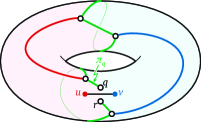
Figure 2: The 2-core $\bar{X}$ of a cut graph $X$ on the torus. Cut paths between red vertices are red, cut paths between blue vertices are blue, and cut paths containing active darts are green.

An edge $e\notin T$ is in $\bar{X}$ if and only if it forms a non-contractible fundamental cycle with $T$ with respect to $\Sigma-r$ or it forms a contractible fundamental cycle with $T$ and lies on $\pi_{q}$ (see Cabello et al. [11, Section 4.1]). We have the following lemmas, the first three of which follow immediately from the symmetry present in the definitions of slack and our perturbation scheme.

Lemma 7.1

Let $d$ be any dart of $T$. We have

$$[slack_{\lambda}(\mathit{rev}(d))]{+\!\!+}\,z(slack_{\lambda}(\mathit{rev}(d)))=[slack_{\lambda}(d)]{+\!\!+}\,z(slack_{\lambda}(d))=0.$$

Lemma 7.2

Let $d$ be an active dart. We have $[slack_{\lambda}(d)]=[\mathit{cycle}(T,d)]+[c^{\prime}(v\mathord{\shortrightarrow}u)]-[\lambda]$.

Lemma 7.3

Let $D=\langle d_{1},d_{2},\dots\rangle$ be a sequence of the active darts in increasing lexicographic order of $[slack_{\lambda}(d_{i})]$. Sequence $D$ is in increasing lexicographic order of $[\mathit{cycle}(T,d_{i})]$ as well.

Lemma 7.4

Suppose a pivot inserts dart $d^{+}$ into the holiest path tree $T$ while removing dart $d^{-}$. Let $d=x\mathord{\shortrightarrow}y$ be any dart where $x$ turns from red to blue while $y$ does not change colors. We have $[\mathit{cycle}(T-d^{-}+d^{+},d)]=[\mathit{cycle}(T,d)]+[\mathit{cycle}(T,d^{+})]$.

• We have $[\mathit{cycle}(T-d^{-}+d^{+},d)]=[\mathit{cycle}(T,d^{+})]+[\mathit{cycle}(T,d)]-[\mathit{cycle}(T,d^{-})]$. However, $[\mathit{cycle}(T,d^{-})]=0$.

Lemma 7.5

Fix an oriented cut path $\xi$, and let $d_{1}$ and $d_{2}$ be darts of $\xi$. Cycles $\gamma_{1}=\mathit{cycle}(T,d_{1})$ and $\gamma_{2}=\mathit{cycle}(T,d_{2})$ are homologous.

• Let $(T,L,C)$ be a tree-cotree decomposition of $G$ where $X$ contains all edges of $C$ and $L$. Without loss of generality, assume the homology signatures $[\cdot]$ are defined using $(T,L,C)$. For any set of dual cycles $\gamma^{*}_{1},\gamma^{*}_{2},\dots$ in $X$ and edge $e$ in $X$, the set of cycles passing through $e$ is determined by which cut path $e$ belongs to. Therefore $[d_{1}]=[d_{2}]$. Because $[d]=0$ for every dart in $T$ and its reversal, we have $[\gamma_{1}]=[\gamma_{2}]$. Lemma 2.1 implies $\gamma_{1}$ and $\gamma_{2}$ are homologous.

Lemma 7.6

Let $\vec{\Pi}=\{\xi_{i_{1}},\xi_{i_{2}},\dots\}$ be the set of oriented cut paths containing darts that are active and whose perturbed slacks have equal homology part. Finally, let $D=\langle d_{1},d_{2},\dots\rangle$ be the sequence of darts within these oriented cut paths in increasing order of perturbed slack. We have $D$ is a subsequence of the blue boundary walk $\bar{P}$. In particular, the darts within any one oriented cut path $\pi\in\Pi$ appear as a consecutive subsequence of $D$.

• We assume $D$ contains at least two darts; otherwise, the proof is trivial. As in the proof of Lemma 6.1, we assume without loss of generality that the drainage $z$ used to define $c^{\prime}$ is defined using cotree $C$ of some tree-cotree decomposition $(T,L,C)$ where $X=L\cup C$. In particular, for each active dart $d$, we have $z(slack_{\lambda}(d))=z(c^{\prime}(d))-z(\lambda)$.

  Let $d_{i_{1}}=x_{1}\mathord{\shortrightarrow}y_{1}$ and $d_{i_{2}}=x_{2}\mathord{\shortrightarrow}y_{2}$ be two distinct active darts in $D$ where $\bar{P}$ includes $d_{i_{1}}$ before $d_{i_{2}}$. Let $P_{1}=\sigma(v,x_{1})\circ x_{1}\mathord{\shortrightarrow}y_{1}\circ\mathit{rev}(\sigma(u,y_{1}))$ and $P_{2}=\sigma(v,x_{2})\circ x_{2}\mathord{\shortrightarrow}y_{2}\circ\mathit{rev}(\sigma(u,y_{2}))$. Let $P_{1}^{\prime}$ be the maximal consecutive subsequence of $P_{1}$ that does not contain darts of $P_{2}$ and define $P_{2}^{\prime}$ similarly. Finally, let $\gamma=P_{2}^{\prime}\circ\mathit{rev}(P_{1}^{\prime})$.

  By assumption, $[\mathit{cycle}(T,d_{i_{1}})]=[\mathit{cycle}(T,d_{i_{2}})]$. Therefore, $[\gamma]=0$. Also, $\gamma$ is simple and non-empty. Together with Lemma 2.1 these facts imply $\gamma$’s dual darts enter a strict subset of faces $F^{\prime}\subseteq F$. Blue boundary walk $\bar{P}$ crosses $\gamma$ only at $\mathit{rev}(d_{i_{1}})$ and $d_{i_{2}}$ before ending at $r$, implying $r\in F^{\prime}$. Lemmas 3.1 and 2.1 imply $z(slack_{\lambda}(d_{i_{2}}))-z(slack_{\lambda}(d_{i_{1}}))=z(c^{\prime}(d_{i_{2}}))-z(c^{\prime}(d_{i_{1}}))=z(c^{\prime}(\gamma))>0$.

Lemma 7.7

Suppose $\lambda_{0}{+\!\!+}\,[\lambda]=c^{\prime}(v\mathord{\shortrightarrow}u)_{0}{+\!\!+}\,[c^{\prime}(v\mathord{\shortrightarrow}u)]$ and $z(\lambda)\leq z(c^{\prime}(v\mathord{\shortrightarrow}u))$. Then, there are no more pivots to perform in the current iteration. In particular, for any dart $d$ with $slack_{\lambda}(d)_{0}=0$, we have $z(slack_{\lambda}(d))>z(c^{\prime}(v\mathord{\shortrightarrow}u))-z(\lambda)$.

• Consider any active dart $d$. The homology and face parts of $slack_{\lambda}(d)$ are equal to the their counterparts in the cost of $\gamma=\sigma(v,x)\circ x\mathord{\shortrightarrow}y\circ\mathit{rev}(\sigma(u,y))\circ u\mathord{\shortrightarrow}v$ according to $c^{\prime}_{\lambda}$. If $[slack_{\lambda}(d)]$ is positive, then $d$ will never be tense in the current iteration. Therefore, $[c^{\prime}_{\lambda}(\gamma)]$ must be zero for $d$ to become tense in the current iteration. However, $[c^{\prime}_{\lambda}(\gamma)]=[c^{\prime}(\gamma)]$. By Lemmas 3.1 and 2.1, $\gamma$ is a boundary circulation. Because $q\mathord{\shortuparrow}r$ is in $\gamma$, the dual darts of $\gamma$ must enter a strict subset of faces $F^{\prime}\subseteq F$ containing $r$. Lemma 3.2 implies $z(c^{\prime}(\gamma))>0$. In particular, $\lambda$ cannot rise high enough to make $d$ tense before it reaches $c^{\prime}(v\mathord{\shortrightarrow}u)$.

7.2 Algorithm Outline

Based on the previous observations, we use the following strategy to compute multiple-source shortest paths. Recall, in each iteration of the multiple-source shortest paths algorithm, we move the source of $T$ between consecutive vertices $u$ and $v$ on $r$. Each iteration begins with the special pivot which sets $\lambda:=-\mathit{dist}_{c^{\prime}}(u,v)$. Now, consider continuously increasing $\lambda$ until it reaches $c^{\prime}(v\mathord{\shortrightarrow}u)$.

We divide the remainder of the iteration into a number of rounds. Over the course of each round, $\lambda_{0}$ remains a static integer while the homology and face parts of $\lambda$ continuously increase. The round ends when either $\lambda=c^{\prime}(v\mathord{\shortrightarrow}u)$ or the homology and face parts of $\lambda$ become infinitely positive. If the latter case occurs, we say the round is fully completed. At the end of fully completed rounds, $\lambda_{0}$ increases by $1$, and the homology and face parts of $\lambda$ become infinitely negative. We perform all pivots necessary to increase $\lambda$ to the end of each round in the order these pivots occur.

An active dart $d$ can pivot into $T$ during the current round only if $slack_{\lambda}(d)_{0}=0$ which implies $[slack_{\lambda}(d)]{+\!\!+}\,z(slack_{\lambda}(d))\geq 0$; the pivot occurs when $\lambda$ becomes large enough that the entire slack vector goes to $\mathrm{𝟎}$. Therefore, we check each active dart $d$ at the moment that $[slack_{\lambda}(d)]{+\!\!+}\,z(slack_{\lambda}(d))=0$ to see if $slack_{\lambda}(d)_{0}=0$ as well. Between pivots, and in accordance with Lemmas 7.2–7.6, we do these checks cut path-by-cut path, first in lexicographic order by $[\mathit{cycle}(T,d)]$, and then in the order they appear along the blue boundary walk $\bar{P}$. We check the active darts within each of the oriented cut paths in order. When we detect a pivot must occur, we perform the pivot and then resume checking darts that still have non-negative homology part to their slack. By Lemma 7.1, the first of these checks occurs on the reversal of the dart just removed from $T$ in the previous pivot. We say a dart $d$ has been passed in the current round when $[slack_{\lambda}(d)]{+\!\!+}\,z(slack_{\lambda}(d))<0$. Each round of checking and pivoting is further broken into three stages as follows:

1. During the first stage, $[\lambda]<[c^{\prime}(v\mathord{\shortrightarrow}u)]$. Following Lemma 7.2, we only check for pivots along cut paths whose darts $d$ have $[\mathit{cycle}(T,d)]<0$. By Lemma 7.7, the current iteration finishes at the end of this stage if $\lambda_{0}=c^{\prime}(v\mathord{\shortrightarrow}u)_{0}$.

2. At the beginning of this stage, the homology and face parts of $\lambda$ are equal to the homology and face parts of $c^{\prime}(v\mathord{\shortrightarrow}u)$. To increase $[\lambda]$, we must check for pivots from active darts $d$ where $[\mathit{cycle}(T,d)]=0$. By Lemma 7.6, darts in $\xi_{q}$ must be checked first. The stage ends immediately after we verify $slack_{\lambda}(d)_{0}>0$ for every dart $d$ in $\xi_{q}$. This stage requires a bit of care, because we cannot afford to explicitly update $\pi_{q}$ after every pivot. This stage most closely resembles how Eisenstat and Klein [24] handle each of the rounds as defined above, because it is the only non-trivial stage when $G$ is a planar graph.

3. At the beginning of this stage, $[\lambda]=[c^{\prime}(v\mathord{\shortrightarrow}u)]$. We now check for pivots along cut paths other than $\pi_{q}$ whose darts $d$ have $[\mathit{cycle}(T,d)]\geq 0$. The end of this stage marks a full completion of the current round.

The rest of this section is organized as follows. In Section 7.3, we go over the data structures used to efficiently implement our algorithm. We then discuss checking for and performing pivots during stages 1 and 3 (Section 7.4) and stage 2 (Section 7.5) separately before discussing the special pivot (Section 7.6) in more detail. We discuss how to efficiently pick which cut path to perform pivot checks on in Section 7.7 before finally analyzing the running time of our algorithm in Section 7.8.

7.3 Data Structures

We begin by describing the data structures used by our algorithm. These data structures extend the ones used by Eisenstat and Klein [24] to work with more general embedded graphs. As a general rule, we explicitly store lots of information about cut paths other than $\pi_{q}$. Handling $\pi_{q}$ requires more care as we do not have time to explicitly maintain it or even remember both of its endpoints at certain moments in the algorithm.

• For each vertex $v\in V$, we store its predecessor dart $pred(v)$ in the shortest path tree $T$.

• For each dual vertex $p\in F$ we store its successor dart $succ(p)$ in an arbitrary dual spanning tree of $X$ rooted at $r$ as well as a boolean $visited(p)$. These values will aid us in maintaining an implicit list of darts along $\xi_{q}$. From the end of stage 2 to immediately before the end of stage 1, $visited(p)$ is True if $succ(p)$ lies on $\xi_{q}$. At the end of stage 1 and between iterations, $visited(p)$ is set to False for every dual vertex $p$. During stage 2, it is only True if $succ(p)$ lies on $\xi_{q}$ and it has been passed in the current round.

• We maintain the unperturbed part of parameter $\lambda$ as $\lambda_{0}$.

• We maintain a reduced cut graph $\tilde{X}$, an embedded graph of genus $g$ with a vertex for every vertex of the 2-core $\bar{X}$ and an edge for every cut path. We refer to vertices and edges of $\tilde{X}$ as cut vertices and cut edges, respectively. As in all embedded graphs, each cut edge $\pi_{i}$ has two cut darts representing the two orientations of $\pi_{i}$. We say a cut dart is active if its oriented cut path contains active darts.

• For each dart $d\in\vec{E}$ we store its unperturbed slack $slack_{0}(d):=slack_{\lambda}(d)_{0}$ as an integer. If $d$’s edge lies on a cut path other than $\pi_{q}$, we also store $\xi(d)$, the cut dart for $d$’s oriented cut path; otherwise, we set $\xi(d)$ to Null.

• Lemma 7.5 implies that for each cut dart $\xi$, there is a unique fundamental cycle homology signature equal to $[d]$ for any dart $d$ in $\xi$’s oriented cut path. We store this value as $[\xi]$. We also store a boolean $passed(\xi)$ that is True if $\xi$ is active and has been passed in the current round. Finally, if $\xi$’s cut path is not $\pi_{q}$, then we store its darts in a list $darts(\xi)$.

• Finally, we maintain a finger $f$ which points to a single dual vertex. When searching $\xi_{q}$ for the next dart to pivot into $T$ we will use $f$ to track our progress.

We begin the algorithm by computing the initial holiest tree $T$ rooted at some vertex $u$ on $r$. We cannot simply apply the linear time algorithm of Henzinger et al. [39], because the perturbed cost of some darts may be negative. Therefore, we begin by computing some shortest path tree rooted at $r$ using the unperturbed costs $c$ in $O(n)$ time. Let $H\subseteq\vec{E}$ be the subset of darts with $\mathrm{𝟎}$ unperturbed slack. The holiest tree uses only darts of $H$. Further, our assumption that $G$ contains no zero-cost cycles guarantees $H$ is acyclic. We compute the holiest tree $T$ from $u$ in $O(gn)$ time using the standard shortest path tree algorithm for directed acyclic graphs on $H$. The initial computation of $T$ is the only time our algorithm will explicitly refer to the face parts of the darts’ perturbed costs. The rest of the data structures can be initialized in $O(gn)$ time. We now discuss how to handle each of the stages as described above. Performing the special pivot is handled last, because the procedure closely resembles pivots performed during these stages.

7.4 Stages 1 and 3

In both stages 1 and 3, we check for and perform pivots using darts on cut paths other than $\pi_{q}$. Suppose we have just performed a pivot or the current stage has just begun. We begin by discussing how to check for pivots.

Checking for pivots

We find the oriented cut path $\xi$ containing the next dart that needs checking for a pivot, assuming one exists. The search can be accomplished by taking a walk along the cut darts of the reduced cut graph that correspond to the blue boundary walk $\bar{P}$. The active cut darts are those whose edges are encountered once during this walk. The oriented cut path we seek corresponds to the first active cut dart $\xi$ in the walk with lexicographically least fundamental cycle homology signature among all unpassed active cut darts. Later, we describe a more efficient way to find $\xi$.

If $\xi=\xi_{q}$, then we have completed stage 1. We take a walk in the dual graph from $q$, following $succ$ pointers until we reach a dual vertex $p$ for which $visited(p)\neq\textsc{True}$. We unset the $visited$ booleans for each dual vertex encountered during the walk. The $visited$ booleans will be fixed to accurately represent $\xi_{q}$ before the next run of stage 1 or 3. If there is no choice for $\xi$, because every active dart has been passed, then we have completed stage 3. We increment $\lambda_{0}$ and unset the $passed$ variables for every cut dart. Then, for each active dart $d$, we decrement $slack_{0}(d)$ and increment $slack_{0}(\mathit{rev}(d))$.

If the current stage is still active, then we check the darts of $darts(\xi)$ in order, performing a pivot if we find a dart $d$ in $darts(\xi)$ with $slack_{0}(d)=0$. Suppose dart $d^{-}$ was removed from $T$ in the previous pivot, we have not yet completed a round since that pivot, and $\mathit{rev}(d^{-})$ is in $darts(\xi)$. In this case, $\mathit{rev}(d^{-})$ is the first dart we check. Otherwise, we start with the first member of $darts(\xi)$. If we find no dart $d$ that can be pivoted into $T$, we set $passed(\xi)$ to True and repeat the search procedure for the next $\xi$.

Performing a pivot

Suppose we decide to pivot dart $d^{+}=x^{+}\mathord{\shortrightarrow}y=o^{+}\mathord{\shortuparrow}p^{+}$ into the holiest tree $T$ while removing dart $d^{-}=x^{-}\mathord{\shortrightarrow}y=o^{-}\mathord{\shortuparrow}p^{-}$. Let $\xi^{+}$ be the cut dart whose oriented cut path contains $d^{+}$. Dart $d^{+}$ lies on some cut path $\pi\neq\pi_{q}$. Cycle $\mathit{cycle}(T-d^{-}+d^{+},d^{-})=\mathit{cycle}(T,d^{+})$ is non-contractible in the surface $\Sigma-r$. Therefore, $d^{-}$ will belong to a new cut path other than $\pi_{q}$ after the pivot. We walk back through the hair of $X$ from $p^{-}$ following $succ$ darts until we encounter a dual vertex $p_{1}$ such that either $\xi(succ(p_{1}))$ is set or $visited(p_{1})$ is set. In the first case, $p_{1}$ lies on a cut path other than $\pi_{q}$. In the latter case, either $p_{1}=q$ or it lies interior to $\pi_{q}$. We also walk forward through the hair from $o^{-}$ following $succ$ darts until we encounter a dual vertex $p_{2}$ lying on some cut path. Note we cannot have both walks end at a $visited$ dual vertex. Otherwise, we will create a contractible dual cycle after adding $d^{-}$’s edge to $X$, implying $T+d^{-}+d^{+}$ is not connected.

After finding $p_{1}$ and $p_{2}$, we modify the reduced cut graph $\tilde{X}$ according to the new cut path from $p_{1}$ to $p_{2}$ that we found. Let $\pi^{-}$ be the new cut edge for this cut path. We add $\pi^{-}$ to $\tilde{X}$, possibly subdividing existing cut edges according to where we found $p_{1}$ and $p_{2}$. When we subdivide cut edges other than the one for $\pi_{q}$, we split the old cut edge’s cut dart’s dart lists. If we subdivide the cut edge for $\pi_{q}$, we unset $visited$ for each dual vertex no longer on $\pi_{q}$ and build new dart lists from scratch for the two new cut darts that are not orientations of the newly shortened $\pi_{q}$. The fundamental cycle homology signature for these new cut darts are initially set to $\mathrm{𝟎}$ to continue respecting the fundamental cycles of $T$. We create new dart lists for both cut darts of $\pi^{-}$ by just including every dart we encountered during the walks and their reversals.

We must then remove the cut edge $\pi^{+}$ for $\xi^{+}$. In a reversal of the above steps, we do a walk from $o^{+}$ along darts of $darts(\mathit{rev}(\xi^{+}))$ until we encounter a dual cut vertex $p_{3}$ of $\bar{X}$. Every dual vertex $p\neq p_{3}$ encountered during the walk becomes a hair of $X$, so we set $succ(p)$ for each of these dual vertices to follow the walk. If $p_{3}$ is an endpoint of $\pi_{q}$, $\pi^{+}$, and exactly one other cut path $\pi$, then the walk continues along $\pi$ until another vertex of $\bar{X}$ is encountered, except now each dual vertex $p$ has both $succ(p)$ set to follow the walk and $visited(p)$ set to True to represent $\pi_{q}$ being enlongated to the new endpoint. A similar walk and setting of dual vertex variables is performed from $p^{+}$ using darts of $darts(\xi^{+})$. We then update $\tilde{X}$ by removing $\pi^{+}$, changing the endpoint of $\pi_{q}$ if necessary, and merging any cut edges sharing degree $2$ vertices of $\tilde{X}$ as well as their lists. Finally, we add $d^{+}$ to $T$ by setting $pred(y):=d^{+}$.

Call each vertex turning from red to blue during the current pivot purple. We must now compute new fundamental cycle homology signatures for cut darts whose darts in $G$ have one purple endpoint. Observe, $[\mathit{cycle}(T,d^{+})]=[\xi^{+}]$. Following Lemma 7.4, we reassign $[\xi]:=[\xi]+[\mathit{cycle}(T,d^{+})]$ for each cut dart $\xi$ whose oriented cut edge contains darts with purple tails but not purple heads. The reversals of these cut darts are assigned the opposite fundamental cycle homology signatures.

Finally, we need to figure out which cut darts have been passed in the current round. Cut dart $\mathit{rev}(d^{-})$ has now become active, because its tail is purple but not its head. Let $\xi^{-}$ be the orientation of $\pi^{-}$ whose oriented cut path contains $d^{-}$. Similar to above, we walk along the $O(g)$ cut darts that correspond to the blue boundary walk $\bar{P}$. By Lemma 7.1, $[slack_{\lambda}(\mathit{rev}(d))]{+\!\!+}\,z(slack_{\lambda}(\mathit{rev}(d)))=0$. Following Lemmas 7.3 and 7.6, we set $passed(\xi):=\textsc{True}$ for each cut dart $\xi$ such that either $[\xi]<[\mathit{rev}(\xi^{-})]$ or $[\xi]=[\mathit{rev}(\xi^{-})]$ and $\xi$ appears earlier in the walk than $\mathit{rev}(\xi^{-})$.

7.5 Stage 2

In stage 2, we check for and performs pivots using darts on $\xi_{q}$. We begin by setting the finger $f:=q$ and then start checking for pivots.

Checking for pivots

We do the following iterative procedure to discover the darts of $\xi_{q}$ and look for pivots. If $\xi(succ(f))$ is set, we have discovered the dual vertex $f$ where $\pi_{q}$ is incident to other cut paths as well as which of the currently stored cut edges contains $f$. We update the reduced cut graph by moving $\pi_{q}$’s endpoint to this newly discovered intersection, subdividing or merging cut edges and cut darts’ dart lists as discussed above. Afterward, the current stage is over.

Suppose $\xi(succ(f))$ is not set. Then, we set $visited(f)$ to true, because $succ(f)$ must lie on $\xi_{q}$. We then check if $slack_{0}(succ(f))=0$. If so, we pivot $succ(f)$ into $T$ as discussed below. If not, we set $f$ to the head of $succ(f)$ to continue the search for the next pivot.

Performing a pivot

Suppose we decide to pivot dart $d^{+}=x^{+}\mathord{\shortrightarrow}y=o^{+}\mathord{\shortuparrow}p^{+}$ into the holiest tree $T$ while removing dart $d^{-}=x^{-}\mathord{\shortrightarrow}y=o^{-}\mathord{\shortuparrow}p^{-}$. We need to reassign $succ$ pointers and unset some $visited$ booleans based on the changing cut path $\pi_{q}$. Dart $\mathit{rev}(d^{-})$ will lie on $\xi_{q}$, because otherwise there will be no path from $o^{+}$ to $r$ in the cut graph. We add $d^{-}$’s edge to $X$ by setting $succ(p^{-}):=\mathit{rev}(d^{-})$. Then, we walk from $p^{-}$, following $succ$ darts until we encounter $o^{+}$. We flip the $visited$ boolean for every dart head encountered on this walk and reverse each dart we walk along to reflect the new route for $\xi_{q}$ through $\mathit{rev}(d^{-})$. Finally, we add $d^{+}$ to $T$ by setting $pred(y):=d^{+}$. We set $f:=p^{-}$ so that $\mathit{rev}(d^{-})$ will be the next dart checked for a pivot.

7.6 The Special Pivot

At the beginning of the iteration, we pivot dart $v\mathord{\shortrightarrow}u=r\mathord{\shortuparrow}q$ into the holiest tree $T$ while removing dart $d^{-}=x^{-}\mathord{\shortrightarrow}v=o^{-}\mathord{\shortuparrow}p^{-}$. We consider two cases for how to handle the special pivot depending on whether it more closely resembles a normal pivot during stages 1 or 3 or a normal pivot during stage 2. We first remark that $\pi_{q}$ may not be known before the special pivot occurs, because all the $visited$ booleans are unset and $q$ was just reassigned for the current iteration. However, $r\mathord{\shortuparrow}q$ lies on a cut path other than $\pi_{q}$ if and only if it did so immediately before reassigning $q$ and performing the special pivot.

Suppose $r\mathord{\shortuparrow}q$ lies on a cut path $\pi^{+}$ other than $\pi_{q}$. In this case, $\pi_{q}$ is actually trivial, because $q$ lies on $\pi^{+}$ as well. In particular, the $visited$ booleans are accurately set to be False everywhere. We update the reduced cut graph by subdividing $\pi^{+}$ and its dart lists to represent the location of $q$. We then follow the same strategy as when we perform a pivot in stage 1 or 3, except we interpret $q$ as $o^{+}$ and $r$ as $p^{+}$ (with this interpretation, $o^{+}\mathord{\shortuparrow}p^{+}$ has the same primal head as $d^{-}$). Of course, we actually set $pred(u):=v$ at the end of the process instead of the other way around. As before, the process ends with $d^{-}$ belonging to a cut path other than $\pi_{q}$. By Lemma 7.1, we have $[slack_{\lambda}(\mathit{rev}(d^{-}))]{+\!\!+}\,z(slack_{\lambda}(\mathit{rev}(d^{-})))=0$. Together with Lemma 7.7, we see the algorithm is now in the middle of stage 1 or stage 3.

Now, suppose $r\mathord{\shortuparrow}q$ is not on a cut path other than $\pi_{q}$. Similar to the strategy for stage 2, we set $succ(p^{-}):=\mathit{rev}(d^{-})$ and then we follow $succ$ darts starting at $p^{-}$ until we reach $q$. We reverse all the $succ$ pointers along the way and set $visited$ to true for each dual vertex at the tail of the new $succ$ pointers to represent the new route $\xi_{q}$ must take through $\mathit{rev}(d^{-})$. We set $pred(u):=v$. By Lemmas 7.1 and 7.7, the algorithm must be in the middle of stage 2, so we set $f:=p^{-}$.

7.7 Searching for Cut Darts

At this point, we have a functioning algorithm that, as argued below, runs in linear time assuming $g$ is a constant. However, the algorithm spends $O(g^{2})$ time every time it starts searching a new dart list of a cut dart. To improve the running time, we maintain an ordered dictionary $\mathcal{A}$ containing active cut darts. The cut darts within $\mathcal{A}$ are sorted first in lexicographic order by their fundamental cycle homology signatures and then in the order their darts of $G^{*}$ appear in the blue boundary walk $\bar{P}$. Dictionary $\mathcal{A}$ will contain at most $O(g)$ cut darts at any one time. It should support insertion and deletion in $O(g\log g)$ time each, finding the first entry in constant time, and finding the successor of any of its current entries in constant time.

Observe that a prefix of the cut darts in $\mathcal{A}$ have been passed. We maintain a pointer to the first member of $\mathcal{A}$ that has not been passed. Therefore, we can select a cut dart along which to do pivot checks in constant time. If no pivots are found, then the pointer is moved to the next member of the dictionary. If there is no next member, then a round has been fully completed. Slack changes are performed in time linear in the number of active darts by touching only darts and their reversals from $\xi_{q}$ and cut darts in $\mathcal{A}$. Afterward, the pointer is moved to the first member of the dictionary. The dictionary is updated after a special pivot that puts the algorithm in stage 1 or 3, after completing a stage 2 that starts immediately after the special pivot, after each pivot in stages 1 and 3, and after any other stage 2 that performs a pivot.

For updates immediately following the special pivot or a stage 2 immediately following it, we remove every cut dart from $\mathcal{A}$, perform the walk in the reduced cut graph corresponding to the blue boundary walk, and add each active cut dart we encounter. The other updates occur when the reduced cut graph is changing. Each cut dart leaving the reduced cut graph is removed from the dictionary $\mathcal{A}$. Then, a walk is done in the new reduced cut graph adding each new cut dart encountered to $\mathcal{A}$. The pointer is updated to the cut dart containing the reverse of the dart of $G$ just pivoted out of $T$.

7.8 Running Time Analysis

Having described how our algorithm is implemented, we turn to bounding its running time. From prior work, we already know there are at most $O(gn)$ pivots [11]. However, we still need a bound on the time spent interacting with individual darts in $X$ that do not get pivoted into $T$ as well as the time spent working with the reduced cut graph and cut dart dictionary $\mathcal{A}$.

Fix a dart $x\mathord{\shortrightarrow}y=o\mathord{\shortuparrow}p$. Let $\langle u_{1},u_{2},\dots,u_{k}\rangle$ be the sequence of sources for the shortest path tree $T$ in order around $r$. We say two paths $P_{1}$ and $P_{2}$ from a vertex on $r$ to $x$ are restricted homotopic with respect to $x\mathord{\shortrightarrow}y$ if there is a homotopy from $P_{1}$ to $P_{2}$ in $\Sigma_{o}=\Sigma-\{o,r\}$ where the first endpoint of the path may move forward or backward along the path $u_{1}\mathord{\shortrightarrow}u_{2}\mathord{\shortrightarrow}\dots\mathord{\shortrightarrow}u_{k-1}$. We have the following lemma.

Lemma 7.8

The shortest path to $x$ in $T$ changes restricted homotopy class with respect to $x\mathord{\shortrightarrow}y$ $O(g)$ times.

• Let $A=\langle\sigma_{1},\sigma_{2},\dots,\sigma_{k}\rangle$ be the sequence of shortest paths to $x$. Suppose $\sigma_{i}$ and $\sigma_{j}$ are restricted homotopic and $j>i$. Let $r[u_{i},u_{j}]$ denote the subpath around $r$ from $u_{i}$ to $u_{j}$. We see $r[u_{i},u_{j}]\circ\sigma_{j}\circ\mathit{rev}(\sigma_{i})$ forms a disk in $\Sigma_{o}$. Because the shortest path from each vertex $u_{i}$ to $x$ is unique, the shortest paths in this set are pairwise non-crossing. In particular, no shortest path between $\sigma_{i}$ and $\sigma_{j}$ can lie in another restricted homotopy class, and each restricted homotopy class is represented by a contiguous subsequence of $A$. Let $A^{\prime}$ be the subsequence containing the first example of each homotopy class. Extend the beginning of each path in $A^{\prime}$ backward along $r$ to $u_{1}$; these extended paths still do not cross. The maximum number of pairwise non-crossing, non-homotopic paths in $\Sigma_{o}$ with common endpoints is $O(g)$ (see Chambers et al. [12, Lemma 2.1]), and this same bound applies to the size of $A^{\prime}$.

The general strategy for bounding the running time of our algorithm is to charge various interactions with darts to changes in the restricted homotopy class of their endpoints. We begin by discussing pivots from stages 1 and 3. The argument for the first case of the special pivot is similar. Suppose we decide to pivot dart $d^{+}=x^{+}\mathord{\shortrightarrow}y=o^{+}\mathord{\shortuparrow}p^{+}$ into the holiest tree $T$ while removing dart $d^{-}=x^{-}\mathord{\shortrightarrow}y=o^{-}\mathord{\shortuparrow}p^{-}$. Recall, a vertex $x$ is purple if it turns from red to blue during a pivot. We may interact with every dart $x\mathord{\shortrightarrow}y$ where $x$ is purple and $y$ is not and their reversals. Cycle $\mathit{cycle}(T,d^{+})$ is non-contractible in the surface $\Sigma-r$. Therefore, for each of these darts $x\mathord{\shortrightarrow}y$, the restricted homotopy class of $x$ relative to $x\mathord{\shortrightarrow}y$ changes. We conclude that we spend $O(gn)$ time total interacting with individual darts during pivots in stages 1 and 3.

We now bound the time spent checking darts for pivots during stages 1 and 3. Suppose we check a dart $d=x\mathord{\shortrightarrow}y$. After the check, dart $d$ has been passed. It will either continue to be passed until the algorithm terminates, it is no longer active, or its unperturbed slack decreases at the end of a round. However, we can only decrease dart $x\mathord{\shortrightarrow}y$’s unperturbed slack at most $c(x\mathord{\shortrightarrow}y)+c(y\mathord{\shortrightarrow}x)$ times before we have to deactivate it and start decreasing the slack of its reversal $y\mathord{\shortrightarrow}x$. Deactivating $d$ requires $x$ being purple, but not $y$, during a pivot, which requires a change in the restricted homotopy class of $x$ relative to $x\mathord{\shortrightarrow}y$ as described above. Overall, we spend at most $O(gL)$ time doing pivot checks during stages 1 and 3.

All other interactions with individual darts occur when preparing for or executing stage 2 of a round, and in every case the $visited$ boolean is switched for one of the darts’ endpoints. We will bound the number of times the $visited$ booleans are set to True at any point in the algorithm. Suppose we set $visited(p)$ to True and let $succ(p)=x\mathord{\shortrightarrow}y=o\mathord{\shortuparrow}p$. If the setting occurs during stage 1 or stage 3, then the restricted homotopy class of $x$ relative to $x\mathord{\shortrightarrow}y$ changes as discussed above. Now suppose the setting occurs during the special pivot or during a pivot in stage 2 where dart $d^{+}=x^{+}\mathord{\shortrightarrow}y=o^{+}\mathord{\shortuparrow}p^{+}$ pivots into holiest tree $T$ while dart $d^{-}=x^{-}\mathord{\shortrightarrow}y=o^{-}\mathord{\shortuparrow}p^{-}$ leaves the tree. Recall, $p$ lies on a walk in the cut graph from $o^{+}$ to $p^{-}$. Every face along this walk, including $p$, is enclosed by $\mathit{cycle}(T,d^{+})$. The restricted homotopy class of $x$ relative to $x\mathord{\shortrightarrow}y$ changes, because the difference between the old shortest path to $x$ and the new shortest path to $x$ encloses $o$ but not $r$. Finally, suppose $visited(p)$ is set to True during stage 2 while checking for pivots along $\xi_{q}$. Similar to above, $visited(p)$ cannot be set again until $succ(p)$ is deactivated during stage 2, $succ(p)$ is deactivated during stage 1 or 3, or the slack of $succ(p)$ is decremented at the end of the round so $visited(p)$ can be unset at the end of stage 1. The first case requires a change of restricted homotopy class as described for when $visited(p)$ is set during a pivot, the second case requires a change of restricted homotopy class as described for darts touched during stages 1 and 3, and the third case can only occur $c(x\mathord{\shortrightarrow}y)+c(y\mathord{\shortrightarrow}x)$ times before a deactivation has to occur anyway. The $visited$ boolean settings, and therefore all individual dart interactions, occur $O(gL)$ times total.

Finally, we must account for the time spent interacting with the reduced cut graph and the ordered dictionary $\mathcal{A}$. There is one $O(g)$-time walk around the reduced cut graph per pivot and $O(gn)$ pivots total, so we spend $O(g^{2}n)$ time doing walks around the reduced cut graph. There are $O(n)$ special pivots, and we can build a fresh copy of $\mathcal{A}$ in $O(g^{2}\log g)$ time after each of them for $O(g^{2}n\log g)$ time total building these fresh copies. A total of $O(gn)$ cut darts enter and leave the reduced cut graph [11, Section 4.2], and each deletion or insertion from $\mathcal{A}$ takes $O(g\log g)$ time, so the individual insertions and deletions during pivots take $O(g^{2}n\log g)$ time total as well.

The overall running time of our algorithm is $O(g(gn\log g+L))$. We have the following theorem.

Theorem 7.9

Let $G=(V,E,F)$ be a graph of size $n$ and genus $g$, let $c:\vec{E}\to\mathbb{N}^{+}$ be a non-negative, integral dart cost function with dart costs summing to $L$, and let $r\in F$ be any face of $G$. We can compute every dart entering and leaving the shortest path trees from each vertex incident to $r$ in order in $O(g(gn\log g+L))$ time.

8 Applications of Linear-time Algorithm

We now turn to applications of the linear-time multiple-source shortest paths algorithm described in the previous section.

8.1 Shortest Path Distances

The above algorithm successfully computes the pivots for multiple-source shortest paths around $r$ in the order that they occur. However, most applications of multiple-source shortest paths are actually concerned with at least a subset of the shortest path distances. Fortunately, this subset of distances is usually structured in a convenient way.

Let $A=\langle u_{1},u_{2},\dots,u_{k_{1}}\rangle$ be the sequence of vertices around $r$, and let $B=\langle v_{1},v_{2},\dots,v_{k_{2}}\rangle$ be the sequence of vertices in an arbitrary walk through $G$. A monotone correspondence $\mathcal{C}$ between $A$ and $B$ is a set of pairs $(u_{i},v_{j})$ where for each $(u_{i},v_{j}),(u_{i^{\prime}},v_{j^{\prime}})\in\mathcal{C}$ with $i^{\prime}\geq i$, we have $j^{\prime}\geq j$. Given a monotone correspondence $\mathcal{C}$, we can easily modify our linear-time algorithm to compute the unperturbed distance from $u_{i}$ to $v_{j}$ for every pair $(u_{i},v_{j})$ appearing in $\mathcal{C}$ with only an $O(k_{2})$ additive increase in the running time. This observation is a generalization of one by Eisenstat and Klein [24, Theorem 4.3] for planar graphs.

We store a variable $\mathit{dist}$ that is initially the unperturbed distance from $u_{1}$ to $v_{1}$. The initial value for $\mathit{dist}$ can be computed in $O(n)$ time after computing the initial holiest tree $T$. As the algorithm runs, we will update $\mathit{dist}$ with the shortest path distance between some $u_{i}$ and $v_{j}$. Suppose an iteration of the algorithm has just ended and we are storing the $u_{i}$ to $v_{j}$ distance. We can compute the unperturbed distance from $u_{i}$ to $v_{j+1}$ as as $\mathit{dist}+c(v_{j}\mathord{\shortrightarrow}v_{j+1})-slack_{0}(v_{j}\mathord{\shortrightarrow}v_{j+1})$ and reassign $\mathit{dist}$ to that value. We repeat this step until we have computed distances for every pair containing $u_{i}$.

Now, suppose we have just performed the special pivot to move the source of $T$ from $u_{i}$ to $u_{i+1}$. After the special pivot, the distance to every vertex in $G$ from the source of $T$ has decreased by the distance from $u_{i}$ to $u_{i+1}$. We decrease $\mathit{dist}$ by that amount. Now, the unperturbed distance from $u_{i+1}$ to some vertex $v_{j}$ increases by $1$ at the end of each fully completed round where $v_{j}$ is red. To easily track if $v_{j}$ is red, we maintain marks on edges appearing an odd number of times along an arbitrary walk from $u_{i+1}$ to $v_{j}$. If there are an odd number of marked edges containing active darts when we increase $\lambda_{0}$, then the unperturbed distance to $v_{j}$ increases by $1$ and we increment $\mathit{dist}$. Otherwise, $\mathit{dist}$ remains unchanged. To maintain these marks for any pair $(u_{i},v_{j})$ we compute an arbitrary $(u_{1},v_{1})$ walk at the beginning of the algorithm. Every time we consider distances to the next vertex along $B$, we flip the mark on the next edge used in $B$’s walk. Every time we perform a special pivot, we flip the mark on the edge for $u_{i}\mathord{\shortrightarrow}u_{i+1}$.

Theorem 8.1

Let $G=(V,E,F)$ be a graph of size $n$ and genus $g$, let $c:\vec{E}\to\mathbb{N}^{+}$ be a non-negative, integral dart cost function with dart costs summing to $L$. Let $r\in F$ be any face of $G$ incident to vertices $A=\langle u_{1},u_{2},\dots,u_{k_{1}}\rangle$ in order, and let $B=\langle v_{1},v_{2},\dots,v_{k_{2}}\rangle$ be the sequence of vertices along an arbitrary walk in $G$. Let $\mathcal{C}$ be an arbitrary monotone correspondence between $A$ and $B$. We can compute the distance from $u_{i}$ to $v_{j}$ for every pair $(u_{i},v_{j})\in\mathcal{C}$ in $O(g(gn\log g+L)+k_{2})$ time.

8.2 The Applications

We can use the algorithm of Theorem 8.1 to easily derive deterministic linear-time algorithms for a variety of problems on unweighted undirected embedded graphs of constant genus. We discuss a few of these problems in this section. For each problem, there is a published algorithm that runs in near-linear time that can use the multiple-source shortest paths algorithm of Cabello et al. [11] in a black box fashion. While Cabello et al. require uniqueness of shortest paths, it is otherwise unnecessary in these algorithms. In every case, the set of shortest path distances required by the algorithm have the form required by Theorem 8.1 with $k_{2}=O(n)$.

We note our multiple-source shortest paths algorithm is not necessary for $g^{O(g)}n$ or (in some cases) $2^{O(g)}n$ time algorithms for these problems, assuming that the input graph is unweighted and undirected. However, we are unaware of any publications stating this observation explicitly. In every case, the use of our linear-time multiple-source shortest paths algorithm results in a substantial decrease in the dependency on $g$.

We give one example of such an algorithm here; the slower algorithms for the other problems use similar ideas. Given an undirected possibly edge weighted graph $G$ and two vertices $s$ and $t$, an $s,t$-cut is a bipartition $(S,T)$ of the vertices such that $s\in S$ and $t\in T$. The capacity of an $s,t$-cut $(S,T)$ is the total number/total weight of all edges with exactly one endpoint in $S$. The minimum $s,t$-cut is the $s,t$-cut of minimum capacity. Chambers et al. [13] reduce the problem of computing a minimum $s,t$-cut in an undirected genus $g$ graph to $g^{O(g)}$ computations of minimum $s^{\prime},t^{\prime}$-cuts in planar graphs of size $O(gn)$. If the input graph is unweighted, then these computations can each be done in $O(gn)$ time each using an algorithm of Weihe [66], yielding a $g^{O(g)}n$ time algorithm for minimum $s,t$-cut in unweighted undirected graphs. We now turn more efficient algorithms that use our linear-time multiple-source shortest paths algorithm instead.

Instead of using the algorithm given above, we can compute minimum $s,t$-cuts in a genus $g$ surface embedded graph using an algorithm of Erickson and Nayyeri [30] that runs $2^{O(g)}$ instances of multiple-source shortest paths in a derived graph of size $2^{O(g)}n$ and genus $2^{O(g)}$.

Theorem 8.2

Let $G=(V,E,F)$ be an unweighted undirected graph of size $n$ and genus $g$, and let $s,t\in V$. There exists a deterministic algorithm that computes a minimum $s,t$-cut of $G$ in $2^{O(g)}n$ time.

A global minimum cut is an $s,t$-cut of minimum capacity across all choices of distinct vertices $s$ and $t$. We can compute global minimum cuts in linear time as well using an algorithm of Erickson et al. [28] with some slight modifications. We replace their use of an algorithm by Chambers et al. [13] for computing minimum weight homologous subgraphs (with coefficients in $\mathbb{Z}_{2}$) with the algorithm of Erickson and Nayyeri [30] for the same problem, plugging in our multiple-source shortest paths algorithm when needed by Erickson and Nayyeri. Again, this results in $2^{O(g)}$ uses of our multiple-source shortest paths algorithm in graphs of size $2^{O(g)}n$ of genus $2^{O(g)}$. Also, we replace Erickson et al.’s [28] constant number of uses of an algorithm by Łącki and Sankowski [50] for global minimum cut in planar graphs with a linear time algorithm for the same problem in unweighted planar graphs by Chang and Lu [16].

Theorem 8.3

Let $G=(V,E,F)$ be an unweighted undirected graph of size $n$ and genus $g$. There exists a deterministic algorithm that computes a global minimum cut of $G$ in $2^{O(g)}n$ time.

Let graph $G$ be embedded in surface $\Sigma$. A non-separating cycle $\gamma$ in $G$ is one for which $\Sigma-\gamma$ is connected. A shortest non-separating or non-contractible cycle is a non-separating or non-contractible cycle with a minimum number of edges or total cost if the edges have costs. We can compute shortest non-separating and non-contractible cycles by simply substituting our multiple-source shortest paths algorithm into the algorithms of Erickson [27] and Fox [34]. Erickson uses $O(g)$ instances of multiple-source shortest paths in derived graphs of size $O(n)$ and genus $O(g)$ to compute a shortest non-separating cycle. Fox uses $O(g^{2}+b)$ instances in derived graphs of size $O(n)$ and genus $O(g)$ to compute a shortest non-contractible cycle when the embedding has $b$ boundary components. Note that these algorithms are actually designed for directed graphs with dart costs, but the undirected case follows from the obvious reduction. For these two problems, there is no other linear time algorithm known for directed graphs with small integer dart costs. However, a running time of $2^{O(g)}n$ is achievable in unweighted undirected graphs by applying Weihe’s [66] minimum $s,t$-cut algorithm as a subroutine in Fox’s [34] modification of Kutz’s [48] original near-linear time algorithm for these problems.

Theorem 8.4

Let $G=(V,E,F)$ be a graph of size $n$ and genus $g$, embedded in a surface with $b$ boundary components, and let $c:\vec{E}\to\mathbb{N}^{+}$ be a positive, integral dart cost function with dart costs summing to $L$. We can compute a shortest non-separating cycle in $G$ in $O(g^{2}(gn\log g+L))$ time and a shortest non-contractible cycle in $G$ in $O((g^{2}+b)g(gn\log g+L))$ time.

Finally, a homology basis is a maximal collection of cycles belonging to linearly independent homology classes with coefficients in $\mathbb{Z}_{2}$. A shortest homology basis is one in which the total number of edges or edge costs is minimized. We combine our algorithm with one by Borradaile et al. [2]. We can compute a shortest homology basis in an unweighted undirected graph by plugging our multiple-source shortest paths algorithm into the algorithm of Borradaile et al. [2]. Their algorithm uses $O((g+b)^{2})$ instances of multiple-source shortest paths in a derived graph of size $O(n)$ and genus $O(g+b)$ when the embedding has $b$ boundary faces.

Theorem 8.5

Let $G=(V,E,F)$ be an unweighted undirected graph of size $n$ and genus $g$, embedded in a surface with $b$ boundary components. There exists a deterministic algorithm that computes a minimum homology basis of $G$ in $O((g+b)^{4}n\log(g+b))$ time.

Acknowledgements.

The authors would like to thank Sergio Cabello, Erin W. Chambers, and Shay Mozes for many helpful discussions. They would also like to thank the anonymous reviewers of the conference version of this paper for their helpful comments on the writing.

References

- [1] C. Berge and A. Ghouilla-Houri. Programming, Games, and Transportation Networks. Methuen & Co, 1965.
- [2] G. Borradaile, E. W. Chambers, K. Fox, and A. Nayyeri. Minimum cycle and homology bases of surface-embedded graphs. J. Comput. Geom., 8(2):58–79, 2017.
- [3] G. Borradaile, D. Eppstein, A. Nayyeri, and C. Wulff-Nilsen. All-pairs minimum cuts in near-linear time for surface-embedded graphs. In Proc. 32nd Intern. Symp. Comput. Geom., pages 22:1–22:16, 2016.
- [4] G. Borradaile and P. Klein. An algorithm for maximum -flow in a directed planar graph. J. ACM, 56(2): 9:1–30, 2009.
- [5] G. Borradaile, P. N. Klein, S. Mozes, Y. Nussbaum, and C. Wulff-Nilsen. Multiple-source multiple-sink maximum flow in directed planar graphs in near-linear time. SIAM J. Comput., 46(4):1280–1303, 2017.
- [6] G. Borradaile, P. Sankowski, and C. Wulff-Nilsen. Min st-cut oracle for planar graphs with near-linear preprocessing time. ACM Trans. Algorithms, 11(3):16:1–16:29, 2015.
- [7] C. Bourke, R. Tewari, and N. V. Vinodchandran. Directed planar reachability is in unambiguous log-space. ACM Trans. Comput. Theory, 1(1):4:1–4:17, 2009.
- [8] U. Brandes and D. Wagner. A linear time algorithm for the arc disjoint Menger problem in planar directed graphs. Algorithmica, 28(1):16–28, 2000.
- [9] O. Busaryev, S. Cabello, C. Chen, T. K. Dey, and Y. Wang. Annotating simplices with a homology basis and its applications. In Proc. 13th Scand. Workshop Algorithm Theory, pages 189–200, 2012.
- [10] S. Cabello. Many distances in planar graphs. Algorithmica, 62(1–2):361–381, 2010.
- [11] S. Cabello, E. W. Chambers, and J. Erickson. Multiple-source shortest paths in embedded graphs. SIAM J. Comput., 42(4):1542–1571, 2013.
- [12] E. W. Chambers, É. Colin de Verdière, J. Erickson, F. Lazarus, and K. Whittlesey. Splitting (complicated) surfaces is hard. Comput. Geom. Theory Appl., 41(1–2):94–110, 2008.
- [13] E. W. Chambers, J. Erickson, and A. Nayyeri. Minimum cuts and shortest homologous cycles. In Proc. 25th Ann. Symp. Comput. Geom., pages 377–385, 2009.
- [14] E. W. Chambers, J. Erickson, and A. Nayyeri. Homology flows, cohomology cuts. SIAM J. Comput., 41(6):1605–1634, 2012.
- [15] E. W. Chambers, K. Fox, and A. Nayyeri. Counting and sampling minimum cuts in genus graphs. Discrete Comput. Geom., 52(3):450–475, 2014.
- [16] H. Chang and H. Lu. Computing the girth of a planar graph in linear time. SIAM J. Comput., 42(3):1077–1094, 2013.
- [17] A. Charnes. Optimality and degeneracy in linear programming. Econometrica, 20(2):160–170, 1952.
- [18] É. Colin de Verdière. Topological algorithms for graphs on surfaces. Habilitation thesis, May 2012.
- [19] W. H. Cunningham. A network simplex method. Math. Program., 11:105–116, 1976.
- [20] G. P. Dantzig, A. Orden, and P. Wolfe. The generalized simplex method for minimizing a linear form under linear inequality constraints. Pacific J. Math., 5:183–195, 1955.
- [21] S. Datta, R. Kulkarni, R. Tewari, and N. V. Vinodchandran. Space complexity of perfect matching in bounded genus bipartite graphs. J. Comput. Syst. Sci., 78(3):765–779, 2012.
- [22] E. W. Dijkstra. A note on two problems in connexion with graphs. Numerische Mathematik, 1:269–271, 1959.
- [23] H. Edelsbrunner and J. L. Harer. Computational Topology: An Introduction. Amer. Math. Soc., 2010.
- [24] D. Eisenstat and P. N. Klein. Linear-time algorithms for max flow and multiple-source shortest paths in unit-weight planar graphs. In Proc. 45th Ann. ACM Symp. Theory Comput., pages 735–744, 2013.
- [25] D. Eppstein. Dynamic generators of topologically embedded graphs. In Proc. 14th Ann. ACM-SIAM Symp. Discrete Algorithms, pages 599–608, 2003.
- [26] J. Erickson. Maximum flows and parametric shortest paths in planar graphs. In Proc. 21st Ann. ACM-SIAM Symp. Discrete Algorithms, pages 794–804, 2010.
- [27] J. Erickson. Shortest non-trivial cycles in directed surface graphs. In Proc. 27th Ann. Symp. Comput. Geom., pages 236–243, 2011.
- [28] J. Erickson, K. Fox, and A. Nayyeri. Global minimum cuts in surface embedded graphs. In Proc. 23rd Ann. ACM-SIAM Symp. Discrete Algorithms, pages 1309–1318, 2012.
- [29] J. Erickson and S. Har-Peled. Optimally cutting a surface into a disk. Discrete Comput. Geom., 31(1):37–59, 2004.
- [30] J. Erickson and A. Nayyeri. Minimum cuts and shortest non-separating cycles via homology covers. In Proc. 22nd Ann. ACM-SIAM Symp. Discrete Algorithms, pages 1166–1176, 2011.
- [31] J. Erickson and K. Whittlesey. Greedy optimal homotopy and homology generators. In Proc. 16th Ann. ACM-SIAM Symp. Discrete Algorithms, pages 1038–1046, 2005.
- [32] J. Erickson and P. Worah. Computing the shortest essential cycle. Discrete Comput. Geom., 44(4):912–930, 2010.
- [33] L. R. Ford and D. R. Fulkerson. Maximal flow through a network. Canad. J. Math., 8(399–404), 1956. First published as Research Memorandum RM-1400, The RAND Corporation, Santa Monica, California, November 19, 1954.
- [34] K. Fox. Shortest non-trivial cycles in directed and undirected surface graphs. In Proc. 24th Ann. ACM-SIAM Symp. Discrete Algorithms, pages 352–364, 2013.
- [35] D. Hartvigsen and R. Mardon. The all-pairs cut problem and the minimum cycle basis problem on planar graphs. SIAM J. Discrete Math., 7(3):403–418, 1994.
- [36] R. Hassin. Maximum flow in planar networks. Inform. Proc. Lett., 13:107, 1981.
- [37] A. Hatcher. Algebraic Topology. Cambridge Univ. Press, 2002.
- [38] M. R. Henzinger and V. King. Randomized fully dynamic graph algorithms with polylogarithmic time per operation. J. ACM, 46(4):502–516, 1999.
- [39] M. R. Henzinger, P. Klein, S. Rao, and S. Subramanian. Faster shortest-path algorithms for planar graphs. J. Comput. Syst. Sci., 55(1):3–23, 1997.
- [40] A. Itai and Y. Shiloach. Maximum flow in planar networks. SIAM J. Comput., 8:135–150, 1979.
- [41] G. F. Italiano, Y. Nussbaum, P. Sankowski, and C. Wulff-Nilsen. Improved algorithms for min cut and max flow in undirected planar graphs. In Proc. 43rd Ann. ACM Symp. Theory Comput., pages 313–322, 2011.
- [42] D. B. Johnson and S. M. Venkatesan. Partition of planar flow networks (preliminary version). In Proc. 24th Ann. IEEE Symp. Found. Comput. Sci., pages 259–264, 1983.
- [43] R. M. Karp and J. B. Orlin. Parametric shortest path algorithms with an application to cyclic staffing. Discrete Appl. Math., 3:37–45, 1981.
- [44] K. Kawarabayashi, P. N. Klein, and C. Sommer. Linear-space approximate distance oracles for planar, bounded-genus and minor-free graphs. In Proc. 38th Int. Colloq. Automata Lang. Prog., volume 6755 of Lecture Notes Comput. Sci., pages 135–146. Springer-Verlag, 2011.
- [45] S. Khuller, J. Naor, and P. Klein. The lattice structure of flow in planar graphs. SIAM J. Discrete Math., pages 477–490, 1993.
- [46] P. Klein. Multiple-source shortest paths in planar graphs. In Proc. 16th Ann. ACM-SIAM Symp. Discrete Algorithms, pages 146–155, 2005.
- [47] P. Klein, S. Mozes, and O. Weimann. Shortest paths in directed planar graphs with negative lengths: A linear-space -time algorithm. ACM Trans. Algorithms, 6(2):article 30, 2010.
- [48] M. Kutz. Computing shortest non-trivial cycles on orientable surfaces of bounded genus in almost linear time. In Proc. 22nd Ann. Symp. Comput. Geom., pages 430–438, 2006.
- [49] J. Łącki, Y. Nussbaum, P. Sankowski, and C. Wulff-Nilsen. Single source - all sinks max flows in planar digraphs. In Proc. 53rd IEEE Symp. Found. Comput. Sci., pages 599–608, 2012.
- [50] J. Łącki and P. Sankowski. Min-cuts and shortest cycles in planar graphs in time. In C. Demetrescu and M. M. Halldórsson, editors, Proc. 19th Ann. Europ. Symp. Algorithms, volume 6942 of Lecture Notes Comput. Sci., pages 155–166. Springer, 2011.
- [51] J. Matuschke and B. Peis. Lattices and maximum flow algorithms in planar graphs. In D. M. Thilikos, editor, Proc. 36th Int. Workshop Graph Theor. Concepts Comput. Sci., number 6410 in Lecture Notes Comput. Sci., pages 324–335. Springer-Verlag, 2010.
- [52] B. Mohar and C. Thomassen. Graphs on Surfaces. Johns Hopkins Univ. Press, 2001.
- [53] S. Mozes, C. Nikolaev, Y. Nussbaum, and O. Weimann. Minimum cut of directed planar graphs in time. In Proc. 29th Ann. ACM-SIAM Symp. Disc. Algo., pages 477–494, 2018.
- [54] S. Mozes and C. Sommer. Exact distance oracles for planar graphs. In Proc. 23rd Ann. ACM-SIAM Symp. Discrete Algorithms, pages 209–222, 2012.
- [55] S. Mozes and C. Wulff-Nilsen. Shortest paths in planar graphs with real lengths in time. In Proc. 18th Ann. Europ. Symp. Algorithms, number 6347 in Lecture Notes Comput. Sci., pages 206–217. Springer-Verlag, 2010.
- [56] K. Mulmuley, U. Vazirani, and V. Vazirani. Matching is as easy as matrix inversion. Combinatorica, 7:105–113, 1987.
- [57] J. R. Munkres. Topology. Prentice-Hall, 2nd edition, 2000.
- [58] J. K. Park and C. A. Philips. Finding minimum-quotient cuts in planar graphs. In Proc. 25th Ann. Symp. Theory Comput., pages 766–775, 1993.
- [59] V. Patel. Determining edge expansion and other connectivity measures of graphs of bounded genus. SIAM J. Comput., 42(3):1113–1131, 2013.
- [60] H. Ripphausen-Lipa, D. Wagner, and K. Weihe. The vertex-disjoint Menger problem in planar graphs. SIAM J. Comput., 26(2):331–349, 1997.
- [61] D. D. Sleator and R. E. Tarjan. A data structure for dynamic trees. J. Comput. Syst. Sci., 26(3):362–391, 1983.
- [62] R. E. Tarjan. Dynamic trees as search trees via euler tours, applied to the network simplex algorithm. Math. Program., 77:169–177, 1997.
- [63] R. E. Tarjan and R. F. Werneck. Self-adjusting top trees. In Proc. 16th Ann. ACM-SIAM Symp. Discrete Algorithms, pages 813–822, 2005.
- [64] R. Tewari and N. V. Vinodchandran. Green’s theorem and isolation in planar graphs. Inf. Comput., 215:1–7, 2012.
- [65] S. M. Venkatesan. Algorithms for network flows. Ph.D. thesis, The Pennsylvania State University, 1983. Cited in [42].
- [66] K. Weihe. Edge-disjoint -paths in undirected planar graphs in linear time. J. Algorithms, 23(1):121–138, 1997.
- [67] K. Weihe. Maximum -flows in planar networks in -time. J. Comput. Syst. Sci., 55(3):454–476, 1997.
- [68] C. Wulff-Nilsen. Minimum cycle basis and all-pairs min cut of a planar graph in subquadratic time. Preprint, December 2009.
- [69] N. E. Young, R. E. Tarjan, and J. B. Orlin. Faster parametric shortest path and minimum balance algorithms. Networks, 21(2):205–221, 1991.
- [70] A. Zomorodian. Topology for Computing. Cambridge Univ. Press, 2005.