Provably Robust Learning-Based Approach for High-Accuracy Tracking Control of Lagrangian Systems

Abstract

Lagrangian systems represent a wide range of robotic systems, including manipulators, wheeled and legged robots, and quadrotors. Inverse dynamics control and feedforward linearization techniques are typically used to convert the complex nonlinear dynamics of Lagrangian systems to a set of decoupled double integrators, and then a standard, outer-loop controller can be used to calculate the commanded acceleration for the linearized system. However, these methods typically depend on having a very accurate system model, which is often not available in practice. While this challenge has been addressed in the literature using different learning approaches, most of these approaches do not provide safety guarantees in terms of stability of the learning-based control system. In this paper, we provide a novel, learning-based control approach based on Gaussian processes (GPs) that ensures both stability of the closed-loop system and high-accuracy tracking. We use GPs to approximate the error between the commanded acceleration and the actual acceleration of the system, and then use the predicted mean and variance of the GP to calculate an upper bound on the uncertainty of the linearized model. This uncertainty bound is then used in a robust, outer-loop controller to ensure stability of the overall system. Moreover, we show that the tracking error converges to a ball with a radius that can be made arbitrarily small. Furthermore, we verify the effectiveness of our approach via simulations on a 2 degree-of-freedom (DOF) planar manipulator and experimentally on a 6 DOF industrial manipulator.

I Introduction

High-accuracy tracking is an essential requirement in advanced manufacturing, self-driving cars, medical robots, and autonomous flying vehicles, among others. To achieve high-accuracy tracking for these complex, typically high-dimensional, nonlinear robotic systems, a standard approach is to use inverse dynamics control [1] or feedforward linearization techniques [2] to convert the complex nonlinear dynamics into a set of decoupled double integrators. Then, a standard, linear, outer-loop controller, e.g., a proportional-derivative (PD) controller, can be used to make the decoupled linear system track the desired trajectory [1]. However, these linearization techniques depend on having accurate system models, which are difficult to obtain in practice.

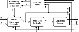
Figure 1: Block diagram of our proposed strategy. GP regression models learn the uncertainty in the linearized model. Using the mean and variance of the GP, one can calculate an upper bound on the uncertainty to be used in a robust, outer-loop controller. The symbol $q$ is the actual position vector, $q_{d}$ is the desired position vector, $a_{q}$ is the commanded acceleration vector, $u$ is the force/torque input vector, and $\eta$ is the uncertainty vector.

To address this problem, robust control techniques have been used for many decades to design the outer-loop controllers to account for the uncertainties in the model [3]. However, the selection of the uncertainty bounds in the robust controller design is challenging. On the one hand, selecting high bounds typically results in a conservative behavior, and hence, a large tracking error. On the other hand, relatively small uncertainty bounds may not represent the true upper bounds of the uncertainties, and consequently, stability of the overall system is not ensured. Alternatively, several approaches have been proposed for learning the inverse system dynamics from collected data where the system models are not available or not sufficiently accurate; see [4, 5, 6, 7]. Combining a-priori model knowledge with learning data has also been studied in [4, 8]. However, these learning approaches typically neglect the learning regression errors in the analysis, and they do not provide a proof of stability of the overall, learning-based control system, which is crucial for safety-critical applications such as medical robots. The limitations of the robust control and the learning-based techniques show the urgent need for novel, robust, learning-based control approaches that ensure both stability of the overall control system and high-accuracy tracking. This sets the stage for the research carried out in this paper.

In this paper, we provide a novel, robust, learning-based control technique that achieves both closed-loop stability and high-accuracy tracking. In particular, we use Gaussian processes (GPs) to approximate the error between the commanded acceleration to the linearized system and the actual acceleration of the robotic system, and then use the predicted mean and variance of the GP to calculate an upper bound on the uncertainty of the linearization. This uncertainty bound is then used in a robust, outer-loop controller to ensure stability of the overall system (see Figure 1). Moreover, we show that using our proposed strategy, the tracking error converges to a ball with a radius that can be made arbitrarily small through appropriate control design, and hence, our proposed approach also achieves high-accuracy tracking. Furthermore, we verify the effectiveness of the proposed approach via simulations on a 2 DOF planar manipulator using MATLAB Simulink and experimentally on a UR10 6 DOF industrial manipulator.

This paper is organized as follows. Section II provides a summary of some recent related work. Section III describes the considered problem, and Section IV provides the proposed approach. Section V derives theoretical guarantees for the proposed approach. Section VI and VII include the simulation and experimental results, and Section VIII concludes the paper.

Notation and Basic Definitions: For a set $S$, $\bar{S}$ denotes its closure and $S^{\circ}$ its interior. The notation $B_{\delta}(y)$ denotes a ball of radius $\delta$ centered at a point $y$. A matrix $P$ is positive definite if it is symmetric and all its eigenvalues are positive. For a vector $x$, $\|x\|$ denotes its Euclidean norm. A function $f(x)$ is smooth if its partial derivatives of all orders exist and are continuous. The solutions of $\dot{x}=f(t,x)$ are uniformly ultimately bounded with ultimate bound $b$ if there exist positive constants $b,~{}c$, and for every $0<a<c$, there exists $T(a,b)\geq 0$ such that $\|x(t_{0})\|\leq a$ implies $\|x(t)\|\leq b$, for all $t\geq(T+t_{0})$, where $t_{0}$ is the initial time instant. A kernel is a symmetric function $k:{\mathcal{A}}\times{\mathcal{A}}\rightarrow{\mathbb{R}}$. A reproducing kernel Hilbert space (RKHS) corresponding to a kernel $k(.,.)$ includes functions of the form $f(a)=\sum_{j=1}^{m}\alpha_{j}k(a,a_{j})$ with $m\in{\mathbb{N}}$, $\alpha_{j}\in{\mathbb{R}}$ and representing points $a_{j}\in{\mathcal{A}}$.

II Related Work

The study of safe learning dates back to the beginning of this century [9]. In [10] and [11], Lyapunov-based reinforcement learning is used to allow a learning agent to safely switch between pre-computed baseline controllers. Then, in [12], risk-sensitive reinforcement learning is proposed, in which the expected return is heuristically weighted with the probability of reaching an error state. In several other papers, including [13], [14] and [15], safe exploration methods are utilized to allow the learning modules to achieve a desired balance between ensuring safe operation and exploring new states for improved performance. In [9], a general framework is proposed for ensuring safety of learning-based control strategies for uncertain robotic systems. In this framework, robust reachability guarantees from control theory are combined with Bayesian analysis based on empirical observations. The result is a safety-preserving, supervisory controller of the learning module that allows the system to freely execute its learning policy almost everywhere, but imposes control actions to ensure safety at critical states. Despite its effectiveness for ensuring safety, the supervisory controller in this approach has no role in reducing tracking errors.

Focusing our attention on safe, learning-based inverse dynamics control, we refer to [16, 17, 18]. In [16], a model reference adaptive control (MRAC) architecture based on Gaussian processes (GPs) is proposed, and stability of the overall control system is proved. While the approach in [16] is based on adaptive control theory, our approach is based on robust control theory. In particular, in [16], the mean of the GP is used to exactly cancel the uncertainty vector, while in our approach, we use both the mean and variance of the GP to learn an upper bound on the uncertainty vector to be used in a robust, outer-loop controller. Hence, unlike [16], in our approach, the uncertainty of the learning module is not only incorporated in the stability analysis but also in the outer-loop controller design. Intuitively, the less certain our GPs are, the more robust the outer-loop controller should be for ensuring safety. When more data is collected and the GPs are more certain, the outer-loop controller can be less conservative for improved performance. While the results of [16] are tested in simulations on a two-dimensional system, we test our results experimentally on a 6 DOF manipulator.

In [17, 18], GPs are utilized to learn the errors in the output torques of the inverse dynamics model online. In [17], the GP learning is combined with a state-of-the-art gradient descent method for learning feedback terms online. The main idea behind this approach is that the gradient descent method would correct for fast perturbations, while the GP is responsible for correcting slow perturbations. This allows for exponential smoothing of the GP hyperparameters, which increases the robustness of the GP at the cost of having slower reactiveness. Nevertheless, [17] does not provide a proof of the robust stability of the closed-loop system. In [18], the variance of the GP prediction is utilized to adapt the parameters of an outer-loop PD controller online, and the uniform ultimate boundedness of the tracking error is proved under some assumptions on the structure of the PD controller (e.g., the gain matrix was assumed to be diagonal, which imposes a decentralized gain control scheme). The results of [18] are verified via simulations on a 2 DOF manipulator.

Our approach differs from [18] in several aspects. First, we do not use an adaptive PD controller in the outer loop, but add a robustness term to the output of the outer-loop controller. Second, while [18] uses the GP to learn the error in the estimated torque from the nominal inverse dynamics, in our approach, we learn the error between the commanded and actual accelerations. This can be beneficial in two aspects: (i) This makes our approach applicable to industrial manipulators that have onboard controllers for calculating the torque and allow the user to only send commanded acceleration/velocity; (ii) this makes our approach also applicable beyond inverse dynamics control of manipulators; indeed, our proposed approach can be applied to any Lagrangian system for which feedforward/feedback linearization can be used to convert the nonlinear dynamics of the system to a set of decoupled double integrators, such as a quadrotor under a feedforward linearization, see Section 5.3 of [19]. Third, while [18] shows uniform ultimate boundedness of the tracking error, it does not provide discussions on the size of the ultimate ball. In this work, we show that using our proposed approach, the size of the ball can be made arbitrarily small through the control design. Fourth, in our approach, we do not impose any assumption on the structure of the outer-loop PD controller and decentralized, outer-loop control is not needed for our proof. Finally, we verify our approach experimentally on a 6 DOF manipulator.

III Problem Statement

In this paper, we consider Lagrangian systems, which represent a wide class of mechanical systems [20]. In what follows, we focus our attention on a class of Lagrangian systems represented by:

$$M(q(t))\ddot{q}(t)+C(q(t),\dot{q}(t))\dot{q}(t)+g(q(t))=u(t),$$ (1)

where $q=(q_{1},\cdots,q_{N})$ is the vector of generalized coordinates (displacements or angles), $\dot{q}=(\dot{q}_{1},\cdots,\dot{q}_{N})$ is the vector of generalized velocities, $u=(u_{1},\cdots,u_{N})$ is the vector of generalized forces (forces or torques), $N$ is the system’s degree of freedom, $M$, $C$, and $g$ are matrices of proper dimensions and smooth functions, and $M(q)$ is a positive definite matrix. Fully-actuated robotic manipulators are an example of Lagrangian systems that can be expressed by (1). Despite focusing our discussion on systems represented by (1), we emphasize that our results in this paper can be easily generalized to a wider class of nonlinear Lagrangian systems for which feedback/feedforward linearization can be utilized to convert the dynamics of the system into a set of decoupled double integrators plus an uncertainty vector.

For the nonlinear system (1) with uncertain matrices $M$, $C$, and $g$, we aim to make the system positions and velocities $(q(t),\dot{q}(t))$ track a desired smooth trajectory $(q_{d}(t),\dot{q}_{d}(t))$. For simplicity of notation, in our discussion, we drop the dependency on time t from $q,~{}q_{d}$, their derivatives, and $u$. Our goal is to design a novel, learning-based control strategy that is easy to interpret and implement, and that satisfies the following desired objectives:

• Robustness: The overall, closed-loop control system satisfies robust stability in the sense that the tracking error has an upper bound under the system uncertainties.

• High-Accuracy Tracking: For feasible desired trajectories, the tracking error converges to a ball around the origin that can be made arbitrarily small through the control design. For the ideal case, where the pre-assumed system parameters are correct, the tracking error should converge exponentially to the origin.

• Adaptability: The proposed strategy should incorporate online learning to continuously adapt to online changes of the system parameters and disturbances.

• Generalizability of the Approach: The proposed approach should be general enough to be also applicable to industrial robots that have onboard controllers for calculating the forces/torques and allow the user to send only commanded acceleration/velocity.

IV Methodology

We present our proposed methodology, and then in the next sections, we show that it satisfies objectives (O1)-(O4).

A standard approach for solving the tracking control problem for (1) is inverse dynamics control. Since $M(q)$ is positive definite by assumption, it is invertible. Hence, it is evident that if the matrices $M$, $C$, and $g$ are all known, then the following inverse dynamics control law

$$u=C(q,\dot{q})\dot{q}+g(q)+M(q)a_{q}$$ (2)

converts the complex nonlinear dynamic system (1) into

$$\ddot{q}=a_{q},$$ (3)

where $a_{q}$ is the commanded acceleration, a new input to the linearized system (3) to be calculated by an outer-loop control law, e.g., a PD controller (see Figure 1). However, the standard inverse dynamics control (2) heavily depends on accurate knowledge of the system parameters. In practice, the matrices $M$, $C$, and $g$ are not perfectly known, and consequently, one has to use estimated values of these matrices $\hat{M}$, $\hat{C}$, and $\hat{g}$, respectively, where $\hat{M}$, $\hat{C}$, and $\hat{g}$ are composed of smooth functions. Hence, in practice, the control law (2) should be replaced with

$$u=\hat{C}(q,\dot{q})\dot{q}+\hat{g}(q)+\hat{M}(q)a_{q}.$$ (4)

Now by plugging (4) into the system model (1), we get

$$\ddot{q}=a_{q}+\eta(q,\dot{q},a_{q}),$$ (5)

where $\eta(q,\dot{q},a_{q})=M^{-1}(q)(\tilde{M}(q)a_{q}+\tilde{C}(q,\dot{q})\dot{q}+\tilde{g}(q))$, with $\tilde{M}=\hat{M}-M$, $\tilde{C}=\hat{C}-C$, and $\tilde{g}=\hat{g}-g$. It can be shown that even if the left hand side (LHS) of (1) has a smooth, unstructured, added uncertainty $E(q,\dot{q})$, e.g., unmodeled friction, (5) is still valid with modified $\eta$. Because of $\eta$, the dynamics (5) resulting from the inverse dynamics control are still nonlinear and coupled. To control the uncertain system (5), on the one hand, robust control methods are typically very conservative, while on the other hand, learning methods do not provide stability guarantees.

Hence, in this paper, we combine ideas from robust control theory with ideas from machine learning, particularly Gaussian processes (GPs) for regression, to provide a robust, learning-based control strategy that satisfies objectives (O1)-(O4). The main idea behind our proposed approach is to use GPs to learn the uncertainty vector $\eta(q,\dot{q},a_{q})$ in (5) online. Following [18], we use a set of $N$ independent GPs, one for learning each element of $\eta$, to reduce the complexity of the regression. It is evident that conditioned on knowing $q,~{}\dot{q}$, and $a_{q}$, one can learn each element of $\eta$ independently from the rest of the elements of $\eta$. A main advantage of GP regression is that it does not only provide an estimated value of the mean $\mu$, but it also provides an expected variance $\sigma^{2}$, which represents the accuracy of the regression model based on the distance to the training data. The punchline here is that one can use both the mean and variance of the GP to calculate an upper bound $\rho$ on $\|\eta\|$ that is guaranteed to be correct with high probability, as we will show later in this section. One can then use this upper bound to design a robust, outer-loop controller that ensures robust stability of the overall system. Hence, our proposed strategy consists of three parts:

(i) Inner-Loop Controller: We use the inverse dynamics control law (4), where $\hat{M}$, $\hat{C}$, and $\hat{g}$ are estimated values of the system matrices from an a-priori model.

(ii) GPs for Learning the Uncertainty: We use a set of $N$ GPs to learn the uncertainty vector $\eta$ in (5). We start by reviewing GP regression [21, 15]. A GP is a nonparametric regression model that is used to approximate a nonlinear function $J(a):{\mathcal{A}}\rightarrow{\mathbb{R}}$, where $a\in{\mathcal{A}}$ is the input vector. The ability of the GP to approximate the function is based on the assumptions that function values $J(a)$ associated with different values of $a$ are random variables, and that any finite number of these variables have a joint Gaussian distribution. The GP predicts the value of the function, $J(a^{*})$, at an arbitrary input $a^{*}\in{\mathcal{A}}$ from a set of $n$ observations $D_{n}:=\{a_{j},\hat{J}(a_{j})\}_{j=1}^{n}$, where $\hat{J}(a_{j})$, $j\in\{1,\cdots,n\}$, are assumed to be noisy measurements of the function’s true values. That is, $\hat{J}(a_{j})=J(a_{j})+\omega^{\prime}$, where $\omega^{\prime}$ is a zero mean Gaussian noise with variance $\sigma_{\omega}^{2}$. Assuming, without loss of generality (w.l.o.g.), a zero prior mean of the GP and conditioned on the previous observations, the mean and variance of the GP prediction are given by:

$$\mu_{n}(a^{*})={\bf k}_{n}(a^{*})({\bf K}_{n}+{\bf I}_{n}\sigma_{\omega}^{2})^{-1}{\bf\hat{J}}_{n},$$ (6)

$$\sigma_{n}^{2}(a^{*})=k(a^{*},a^{*})-{\bf k}_{n}(a^{*})({\bf K}_{n}+{\bf I}_{n}\sigma_{\omega}^{2})^{-1}{\bf k}_{n}^{T}(a^{*}),$$ (7)

respectively, where ${\bf\hat{J}}_{n}=[\hat{J}(a_{1}),\cdots,\hat{J}(a_{n})]^{T}$ is the vector of observed, noisy function values. The matrix ${\bf K}_{n}\in{\mathbb{R}}^{n\times n}$ is the covariance matrix with entries $[{\bf K}_{n}]_{(i,j)}=k(a_{i},a_{j})$, $i,~{}j\in\{1,\cdots,n\}$, where $k(a_{i},a_{j})$ is the covariance function defining the covariance between two function values $J(a_{i}),~{}J(a_{j})$ (also called the kernel). The vector ${\bf k}_{n}(a^{*})=[k(a^{*},a_{1}),\cdots,k(a^{*},a_{n})]$ contains the covariances between the new input and the observed data points, and ${\bf I}_{n}\in{\mathbb{R}}^{n\times n}$ is the identity matrix. The tuning of the GP is typically done through the selection of the kernel function and the tuning of its hyperparameters. For information about different standard kernel functions, please refer to [21].

We next discuss our implementation of the GPs. The GPs run in discrete time with sampling interval $T_{s}$. At a sampling instant $k$, the inputs to each GP regression model are the same $(q(k),\dot{q}(k),{a_{q}}(k))$, and the output is an estimated value of an element of the $\eta$ vector at $k$. For the training data for each GP, $n$ observations of $(q,\dot{q},a_{q})$ are used as the labeled input together with $n$ observations of an element of the vector $\ddot{q}-a_{q}+{\bf\omega}_{v}$ as the labeled output, where ${\bf\omega}_{v}\in{\mathbb{R}}^{N}$ is Gaussian noise with zero mean and variance $diag(\sigma_{\omega_{1}}^{2},\cdots,\sigma_{\omega_{N}}^{2})$; see (5). For selecting the $n$ observations, we use the oldest point (OP) scheme for simplicity; this scheme depends on removing the oldest observation to accommodate for a new one [16]. We use the squared exponential kernel

$$k(a_{i},a_{j})=\sigma_{\eta}^{2}e^{-\frac{1}{2}(a_{i}-a_{j})^{T}\bar{M}^{-2}(a_{i}-a_{j})},$$ (8)

which is parameterized by the hyperparameters: $\sigma_{\eta}^{2}$, the prior variance, and the positive length scales $l_{1},\cdots,l_{3N}$ which are the diagonal elements of the diagonal matrix $\bar{M}$. Hence, the expected mean and variance of each GP can be obtained through equations (6)-(8). Guidelines for tuning the GP hyperparameters $\sigma_{\omega}^{2},\sigma_{\eta}^{2},l_{1},\cdots,l_{3N}$ can be found in [15].

As stated before, a main advantage of GP regression is that the GP provides a variance, which represents the accuracy of the regression model based on the distance between the new input and the training data. One can then use the predicted mean and variance of the GP to provide a confidence interval around the mean that is guaranteed to be correct with high probability. There are several comprehensive studies in the machine learning literature on calculating these confidence intervals. For completeness, we review one of these results, particularly Theorem 6 of [21]. Let $a_{aug}=(q,\dot{q},a_{q})$, and $\eta_{i}(a_{aug})$ denote the $i$-th element of the unknown vector $\eta$.

Assumption IV.1

The function $\eta_{i}(a_{aug})$, $i\in\{1,\cdots,N\}$, has a bounded RKHS norm $\|\eta_{i}\|_{k}$ with respect to the covariance function $k(a,a^{\prime})$ of the GP, and the noise $\omega_{i}$ added to the output observations, $i\in\{1,\cdots,N\}$, is uniformly bounded by $\bar{\sigma}$.

The RKHS norm is a measure of the function smoothness, and its boundedness implies that the function is well-behaved in the sense that it is regular with respect to the kernel [21]. Intuitively, Assumption IV.1 does not hold if the uncertainty $\eta$ is discontinuous, e.g., discontinuous friction.

Lemma IV.1 (Theorem 6 of [21])

Suppose that Assumption IV.1 holds. Let $\delta_{p}\in(0,1)$. Then, $\Pr\{\forall a_{aug}\in{\mathcal{A}},\|\mu(a_{aug})-\eta_{i}(a_{aug})\|\leq\beta^{1/2}\sigma(a_{aug})\}\geq 1-\delta_{p}$, where $\Pr$ stands for the probability, ${\mathcal{A}}\subset{\mathbb{R}}^{3N}$ is compact, $\mu(a_{aug}),~{}\sigma^{2}(a_{aug})$ are the GP mean and variance evaluated at $a_{aug}$ conditioned on $n$ past observations, and $\beta=2\|\eta_{i}\|_{k}^{2}+300\gamma\ln^{3}((n+1)/{\delta}_{p})$. The variable $\gamma\in{\mathbb{R}}$ is the maximum information gain and is given by $\gamma=\max_{\{a_{aug,1},\cdots,a_{aug,n+1}\}\in{\mathcal{A}}}0.5~{}\log(\det(I+\bar{\sigma}^{-2}{\bf K}_{n+1}))$, where $\det$ is the matrix determinant, $I\in{\mathbb{R}}^{(n+1)\times(n+1)}$ is the identity matrix, ${\bf K}_{n+1}\in{\mathbb{R}}^{(n+1)\times(n+1)}$ is the covariance matrix given by $[{\bf K}_{n+1}]_{(i,j)}=k(a_{aug,i},a_{aug,j})$, $i,~{}j\in\{1,\cdots,n+1\}$.

Finding the information gain maximizer can be approximated by an efficient greedy algorithm [21]. Indeed, $\gamma$ has a sublinear dependence on $n$ for many commonly used kernels, and can be numerically approximated by a constant [18].

The punchline here is that we know from Lemma IV.1 that one can define for each GP a confidence interval around the mean that is guaranteed to be correct for all points $a_{aug}\in{\mathcal{A}}$, a compact set, with probability higher than $(1-\delta_{p})$, where $\delta_{p}$ is typically picked very small. Let $\mu_{k,i}$ and $\sigma_{k,i}^{2}$ represent the expected mean and variance of the $i$-th GP at the sampling instant $k$, respectively, and let $\beta_{i}$ denote the $\beta$ parameter in Lemma IV.1 of the $i$-th GP, where $i\in\{1,\cdots,N\}$. We select the upper bound on the absolute value of $\eta_{i}$ at $k$ to be

$$\rho_{k,i}(\mu_{k,i},\sigma_{k,i})=\max(|\mu_{k,i}-\beta_{i}^{1/2}\sigma_{k,i}|,|\mu_{k,i}+\beta_{i}^{1/2}\sigma_{k,i}|).$$ (9)

Then, a good estimate of the upper bound on $\|\eta\|$ at $k$ is

$$\rho_{k}=\sqrt{\rho_{k,1}(\mu_{k,1},\sigma_{k,1})^{2}+\cdots+\rho_{k,N}(\mu_{k,N},\sigma_{k,N})^{2}}.$$ (10)

(iii) Robust, Outer-Loop Controller: We use the estimated upper bound $\rho_{k}$ to design a robust, outer-loop controller. In particular, for a smooth, bounded desired trajectory $q_{d}(t)$, we use the outer-loop control law

$$a_{q}(t)=\ddot{q}_{d}(t)+K_{P}(q_{d}(t)-q(t))+K_{D}(\dot{q}_{d}(t)-\dot{q}(t))+r(t),$$ (11)

where $K_{P}\in{\mathbb{R}}^{N\times N}$ and $K_{D}\in{\mathbb{R}}^{N\times N}$ are the proportional and derivative matrices of the PD control law, respectively, and $r\in{\mathbb{R}}^{N}$ is an added vector to the PD control law that will be designed to achieve robustness. Let $e(t):=(q(t)-q_{d}(t),\dot{q}(t)-\dot{q}_{d}(t))$ denote the tracking error vector. From (11) and (5), it can be shown that the tracking error dynamics are

$$\dot{e}(t)=Ae(t)+B(r(t)+\eta(q(t),\dot{q}(t),a_{q}(t))),$$ (12)

where

$$A=\left[\begin{array}[]{cc}0&I\\ -K_{P}&-K_{D}\end{array}\right]\in{\mathbb{R}}^{2N\times 2N},~{}~{}B=\left[\begin{array}[]{rr}0\\ I\end{array}\right]\in{\mathbb{R}}^{2N\times N},$$ (13)

and $I\in{\mathbb{R}}^{N\times N}$ is the identity matrix. From (12) and (13), it is clear that the controller matrices $K_{P}$ and $K_{D}$ should be designed to make $A$ a Hurwitz matrix.

We now discuss how to design the robustness vector $r(t)$. To that end, let $P\in{\mathbb{R}}^{2N\times 2N}$ be the unique positive definite matrix satisfying $A^{T}P+PA=-Q$, where $Q\in{\mathbb{R}}^{2N\times 2N}$ is a positive definite matrix. We define $r(t)$ as follows

$$r(t)=\begin{cases}-\rho(t)\frac{B^{T}Pe(t)}{\|B^{T}Pe(t)\|}\text{~{}~{}~{}~{}$\|B^{T}Pe(t)\|>\epsilon$,}\\ -\rho(t)\frac{B^{T}Pe(t)}{\epsilon}\text{~{}~{}~{}~{}~{}~{}$\|B^{T}Pe(t)\|\leq\epsilon$,}\end{cases}$$ (14)

where $\rho(t)\in{\mathbb{R}}$ is the last received upper bound on $\|\eta\|$ from the GPs, i.e., we use

$$\rho(t)=\rho_{k},\forall t\in[kT_{s},(k+1)T_{s}),$$ (15)

and $\epsilon$ is a small positive number. It should be noted that $\epsilon$ is a design parameter that can be selected to ensure high-accuracy tracking, as we will discuss in the next section.

V Theoretical Guarantees

After discussing the proposed strategy, we now justify that it satisfies both robust stability and high-accuracy tracking. To that end, we require the following reasonable assumption:

Assumption V.1

The GPs run at a sufficiently fast sampling rate such that the calculated upper bound on $\|\eta\|$ is accurate between two consecutive sampling instants.

We impose another assumption to ensure that the added robustness vector $r(t)$ will not cause the uncertainty vector norm $\|\eta(q(t),\dot{q}(t),a_{q}(t))\|$ to blow up. It is easy to show that the uncertainty function $\eta(q,\dot{q},a_{q})$ is smooth, and so $\|\eta\|$ attains a maximum value on any compact set in its input space $(q,\dot{q},a_{q})$. However, since from (11) and (14), $a_{q}$ is a function of $\rho(t)$, an upper bound on $\|\eta\|$, one still needs to ensure the boundedness of $\|\eta\|$ for bounded $q,~{}\dot{q}$ or bounded tracking error $e$. Hence, we present the following assumption.

Assumption V.2

For a given, smooth, bounded desired trajectory $(q_{d}(t),\dot{q}_{d}(t))$, there exists $\bar{\rho}>0$ such that $\|\eta\|\leq\bar{\rho}$ for each $e\in D$, where $D$ is a compact set containing $\{e\in{\mathbb{R}}^{2N}:e^{T}Pe\leq e(0)^{T}Pe(0)\}$, and $e(0)$ is the initial tracking error.

We now justify that Assumption V.2 is reasonable. In particular, we show that the assumption is satisfied for small uncertainties in the inertia matrix $M(q)$ [1]. In this discussion, we suppose that $\rho(t)$ in (14) satisfies $\rho(t)\leq\|\eta(t)\|+c$, where $c$ is a positive scalar, and study whether imposing $r(t)$ into (11) can make $\|\eta(t)\|$ blow up. Recall that $\eta(q,\dot{q},a_{q})=M^{-1}(q)(\tilde{M}(q)a_{q}+\tilde{C}(q,\dot{q})\dot{q}+\tilde{g}(q))$. From (11), we have $\eta(q,\dot{q},a_{q})=M^{-1}(q)(\tilde{M}(q)r+\tilde{M}(q)(\ddot{q}_{d}+K_{P}(q_{d}-q)+K_{D}(\dot{q}_{d}-\dot{q}))+\tilde{C}(q,\dot{q})\dot{q}+\tilde{g}(q))$. It is evident that $\|\eta\|\leq\|M^{-1}(q)\tilde{M}(q)\|\|r\|+\|T_{b}(q,\dot{q},q_{d},\dot{q}_{d},\ddot{q}_{d})\|$, where $T_{b}=M^{-1}(q)(\tilde{M}(q)(\ddot{q}_{d}+K_{P}(q_{d}-q)+K_{D}(\dot{q}_{d}-\dot{q}))+\tilde{C}(q,\dot{q})\dot{q}+\tilde{g}(q))$. From (14), it is easy to verify $\|r(t)\|\leq\|\rho(t)\|=\rho(t)$, and so $\|r(t)\|\leq\|\eta(t)\|+c$. Hence, $\|\eta\|\leq\|M^{-1}(q)\tilde{M}(q)\|\|\eta\|+\|M^{-1}(q)\tilde{M}(q)\|c+\|T_{b}\|$. Now if the uncertainty in the matrix $M(q)$, $\tilde{M}(q)$, is sufficiently small such that $\|M^{-1}(q)\tilde{M}(q)\|<1$ is satisfied, then $\|\eta\|\leq\frac{1}{1-\|M^{-1}(q)\tilde{M}(q)\|}(\|M^{-1}(q)\tilde{M}(q)\|c+\|T_{b}(q,\dot{q},q_{d},\dot{q}_{d},\ddot{q}_{d}\|)$.

Since $q_{d},~{}\dot{q}_{d},~{}\ddot{q}_{d}$ are all bounded by assumption, if $e(t)\in D$, a compact set, then $q(t),~{}\dot{q}(t)$ are also bounded. It is easy to show that there exists a fixed upper bound $\bar{\rho}$ on $\|\eta\|$ that is valid for each $e\in D$, and Assumption V.2 is satisfied.

Remark V.1

We have shown that if the uncertainty in the matrix $M(q)$, $\tilde{M}(q)$, is sufficiently small such that $\|M^{-1}(q)\tilde{M}(q)\|<1$ is satisfied, then Assumption V.2 holds. This argument is true even if we have large uncertainties in the other system matrices, $C(q,\dot{q})$ and $g(q)$. As indicated in Chapter 8 of [1], if the bounds on $\|M\|$ are known ($\underline{m}\leq\|M\|\leq\overline{m}$), then one can always select $\hat{M}$ such that $\|M^{-1}(q)\tilde{M}(q)\|<1$ is satisfied. In particular, by selecting $\hat{M}=\frac{\overline{m}+\underline{m}}{2}I$, where $I$ is the identity matrix, it can be shown that $\|M^{-1}(q)\tilde{M}(q)\|\leq\frac{\overline{m}-\underline{m}}{\overline{m}+\underline{m}}<1$. Consequently, it is not difficult to satisfy the condition $\|M^{-1}(q)\tilde{M}(q)\|<1$ in practice, and Assumption V.2 is not restrictive.

From Assumption V.2, we know that $\|\eta(t)\|\leq\bar{\rho}$ if $e(t)\in D$, and consequently, it is reasonable to saturate any estimate of $\rho(t)$ beyond $\bar{\rho}$. Hence, we suppose that the estimation of $\rho$ is slightly modified to be

$$\rho(t)=\min(\rho_{GP}(t),\bar{\rho}),$$ (16)

where $\rho_{GP}(t)$ is the upper bound on the uncertainty norm, $\|\eta\|$, calculated from the GPs in (9), (10), and (15). It is straightforward to show that with the choice of $\rho(t)$ in (16) and for bounded smooth trajectories, the condition $e(t)\in D$ for all $t\geq 0$ implies that $a_{q}(t)$ in (11) is always bounded, and so $a_{aug}=(q,\dot{q},a_{q})$ always lies in a compact set. To be able to provide theoretical guarantees, we also assume w.l.o.g. that the small positive number $\epsilon$ in (14) is selected sufficiently small such that

$$\sqrt{\frac{\epsilon\bar{\rho}}{2\lambda_{min}(Q)}}\ll\delta_{1},$$ (17)

where $\delta_{1}>0$ is such that $B_{\delta_{1}}(0)\subset\{e\in{\mathbb{R}}^{2N}:e^{T}Pe<e(0)^{T}Pe(0)\}$, and $\lambda_{min}(Q)>0$ is the smallest eigenvalue of the positive definite matrix $Q$.

Based on Assumptions IV.1, V.1 and V.2, we provide the following main result.

Theorem V.1

Consider the Lagrangian system (1) and a smooth, bounded desired trajectory $(q_{d}(t),\dot{q}_{d}(t))$. Suppose that Assumptions IV.1, V.1, and V.2 hold. Then, the proposed, robust, learning-based control strategy in (4), (11), and (14), with the uncertainty upper bound $\rho$ calculated by (16) and the design parameter $\epsilon$ satisfying (17), ensures with high probability of at least $(1-\delta_{p})^{N}$ that the tracking error $e(t)$ is uniformly ultimately bounded with an ultimate bound that can be made arbitrarily small through the selection of the design parameter $\epsilon$.

Proof:

From Assumption V.2, we know that $\|\eta(t)\|\leq\bar{\rho}$ when $e(t)\in D$, where $D$ is a compact set containing $\{e\in{\mathbb{R}}^{2N}:e^{T}Pe\leq e(0)^{T}Pe(0)\}$. In the first part of the proof, we assume that the upper bound $\rho_{GP}(t)$ calculated by (9), (10) and (15) is a correct upper bound on $\|\eta(t)\|$ when $e(t)\in D$. Thus, in the first part of the proof, we know that $\rho(t)$ calculated by (16) is a correct upper bound on $\|\eta(t)\|$ when $e(t)\in D$, and we use Lyapunov stability analysis to prove that $e(t)$ is uniformly ultimately bounded. Then, in the second part of the proof, we use Lemma IV.1 to evaluate the probability of satisfying the assumption that $\rho_{GP}(t)$ is a correct upper bound on $\|\eta(t)\|$ when $e(t)\in D$, and hence, the probability that the provided guarantees hold.

The first part of the proof closely follows the proof of the effectiveness of the robust controller in Theorem 3 of Chapter 8 of [1], and we include the main steps of the proof here for convenience. Consider a candidate Lyapunov function $V(e)=e^{T}Pe$. From (12), it can be shown that $\dot{V}=-e^{T}Qe+2w^{T}(\eta+r)$, where $w=B^{T}Pe$. Then, from (14), we need to study two cases.

For the case where $\|w\|>\epsilon$, we have

$$w^{T}(\eta+r) =w^{T}(\eta-\rho\frac{w}{\|w\|})=w^{T}\eta-\rho\|w\|$$

$$\leq\|\eta\|\|w\|-\rho\|w\|$$

from the Cauchy-Schwartz inequality. Since $\{e\in{\mathbb{R}}^{2N}:e^{T}Pe\leq e(0)^{T}Pe(0)\}\subset D$ by definition and from Assumption V.2, we know that $\|\eta\|\leq\bar{\rho}$. Also, by our assumption in this part of the proof, $\|\eta\|\leq\rho_{GP}$. Then, from (16), $\|\eta\|\leq\rho$, and $w^{T}(\eta+r)\leq 0$. Thus, for this case, $\dot{V}\leq-e^{T}Qe$, which ensures exponential decrease of the Lyapunov function.

Next, consider the case where $\|w\|\leq\epsilon$. If $w=0$, then $\dot{V}=-e^{T}Qe<0$. Then, for $\|w\|\leq\epsilon$ and $w\neq 0$, it is easy to show

$$\dot{V}=-e^{T}Qe+2w^{T}(\eta+r)\leq-e^{T}Qe+2w^{T}(\rho\frac{w}{\|w\|}+r).$$

From (14), we have

$$\dot{V}\leq-e^{T}Qe+2w^{T}(\rho\frac{w}{\|w\|}-\rho\frac{w}{\epsilon}).$$

It can be shown that the term $2w^{T}(\rho\frac{w}{\|w\|}-\rho\frac{w}{\epsilon})$ has a maximum value of $(\epsilon\rho)/2$ when $\|w\|=\epsilon/2$. Thus, $\dot{V}\leq-e^{T}Qe+(\epsilon\rho)/2$. From (16), $\rho\leq\bar{\rho}$, and consequently $\dot{V}\leq-e^{T}Qe+(\epsilon\bar{\rho})/2$. If the condition $e^{T}Qe>(\epsilon\bar{\rho})/2$ is satisfied, then $\dot{V}<0$. Since $Q$ is positive definite by definition, then $e^{T}Qe\geq\lambda_{min}(Q)\|e\|^{2}$, where $\lambda_{min}(Q)>0$ is the smallest eigenvalue of $Q$. Hence, if $\lambda_{min}(Q)\|e\|^{2}>(\epsilon\bar{\rho})/2$, then $\dot{V}<0$. Thus, the Lyapunov function is strictly decreasing if $\|e\|>\sqrt{\frac{\epsilon\bar{\rho}}{2\lambda_{min}(Q)}}$. Let $B_{\delta}$ be the ball around the origin of radius $\delta:=\sqrt{\frac{\epsilon\bar{\rho}}{2\lambda_{min}(Q)}}$, $S_{\delta}$ be a sufficiently small sublevel set of the Lyapunov function V satisfying $\bar{B}_{\delta}\subset S_{\delta}^{\circ}$, and $B_{c}$ be the smallest ball around the origin satisfying $S_{\delta}\subset\bar{B}_{c}$. Since the Lyapunov function $V$ is strictly decreasing outside $\bar{B}_{\delta}$, the tracking error $e(t)$ eventually reaches and remains in $S_{\delta}\subset\bar{B}_{c}$, and so the tracking error $e(t)$ is uniformly ultimately bounded, and its ultimate bound is the radius of $B_{c}$. Note that from (17), $B_{\delta}\subset\{e\in{\mathbb{R}}^{2N}:e^{T}Pe<e(0)^{T}Pe(0)\}\subset D$, and $\rho$ is a correct upper bound on $\|\eta\|$. One can see that $\delta$ and hence the radius of $B_{c}$ depend on the choice of the design parameter $\epsilon$. Indeed, $\epsilon$ can be selected sufficiently small to make $B_{\delta}$ and $B_{c}$ arbitrarily small.

In the second part of the proof, we calculate the probability of our assumption in the first part that $\rho_{GP}(t)$ is a correct upper bound on $\|\eta(t)\|$ when $e(t)\in D$. Recall that $e(t)\in D$ implies that $a_{aug}(t)$ is in a compact set, as discussed immediately after (16). From Assumption V.1, our problem reduces to calculating the probability that $\rho_{GP}$ is a correct upper bound on $\|\eta\|$ for all the sampling instants. Using the confidence region proposed in Lemma IV.1 for calculating the upper bound on the absolute value of each element of $\eta$, and under Assumption IV.1, the probability that this upper bound is correct for all samples is higher than $(1-\delta_{p})$ from Lemma IV.1. Since the $N$ GPs are independent and the added noise to the output observations ${\bf\omega}_{v}$ is uncorrelated, then the probability that the upper bounds on the absolute values of all the elments of $\eta$, and hence the upper bound on $\|\eta(t)\|$, are correct is higher than $(1-\delta_{p})^{N}$. ∎

Remark V.2

Although in practice it is difficult to estimate the upper bound $\bar{\rho}$ on $\|\eta\|$ used in (16), one can be conservative in this choice. Unlike robust control techniques that keep this conservative bound unchanged, (16) would relax the upper bound $\bar{\rho}$ when the GPs learn a lower upper bound from collected data. Having a less-conservative upper bound $\rho$ results in a lower tracking error. It can be shown that if $\rho(t)\leq\rho^{\prime}<\bar{\rho}$ for all $t$, then the tracking error will converge to an ultimate ball $B_{c^{\prime}}$ smaller than $B_{c}$.

Remark V.3

In theory, $\epsilon$ can be selected sufficiently small to ensure arbitrarily accurate tracking as shown in the proof of Theorem V.1. Achieving that for cases with large uncertainties may be limited by the actuation limits of the robots. Incorporating the actuation limits in the theoretical analysis is an interesting point for future research.

VI Simulation Results

The proposed approach is first verified via simulations on a 2 DOF planar manipulator using MATLAB Simulink

We use the robot dynamics (1) for the system, where $M$, $C$, and $g$ are as defined in Chapter 7 of [1]. For the system parameters, a value of $1~{}\mathrm{kg}$ is used for each link mass and $1~{}\mathrm{kg\cdot{m^{2}}}$ for each link inertia. The length of the first link is $2~{}\mathrm{m}$ and that of the second link is $1~{}\mathrm{m}$. The joints are assumed to have no mass and are not affected by friction. Then, it is assumed that these parameters are not perfectly known. Thus, in the inverse dynamics controller (4), we use parameters with different levels of uncertainties. The desired trajectories are sinusoidal trajectories with different amplitudes and frequencies. All the simulation runs are initialized at zero initial conditions.

We use $2$ GPs to learn the uncertainty vector $\eta$ in (5). Each GP uses the squared exponential kernel parameterized with $\sigma_{\eta,{i}}=1$, $\sigma_{\omega,{i}}=0.001$, and $l_{j,i}=0.5$, for all $j\in\{1,\cdots,6\}$ and $i\in\{1,2\}$. The GPs run at $10~{}\mathrm{Hz}$ and use the past $n=20$ observations for prediction. To generate confidence intervals, we use $[\mu_{k}-3\sigma_{k},\mu_{k}+3\sigma_{k}]$, which is simple to implement and found to be effective in practice [15]. For the robust controller, we use $\epsilon=0.001$. We set the upper bound $\bar{\rho}$ in (16) to be a very high positive number to evaluate the effectiveness of the upper bound estimated by the GPs.

A sequence of 12 trajectories was run for 3 different cases of model uncertainty. Each of the three cases makes the $\hat{M}$ matrix differ from the $M$ matrix by using values for the estimated link masses that differ from the true link mass values. In particular, in the three uncertainty cases, the estimated mass differs from the actual mass by $10\%$, $20\%$, and $30\%$ for each link, respectively.

The tracking performance was compared between four controllers: a nominal controller with no robust control, a robust controller with a fixed upper bound on the uncertainty norm $\rho=1000$, a learning-based inverse dynamics controller in which GPs are used to learn the error of the nominal inverse model at the torque level $\Delta u$ and a non-robust outer-loop controller is used, and our proposed robust learning controller. The root-mean-square (RMS) error of the joint angles was averaged over the 12 trajectories, and is presented for each controller and uncertainty case in Table I.

TABLE I: Average RMS Tracking Error (in rad) Over 12 Trajectories for Different Controllers on a 2 DOF Manipulator

Uncertainty	Nominal	Fixed Robust	Learning $\Delta u$	Robust Learning
$10\%$	0.1554	0.0476	0.0190	0.0082
$20\%$	0.2793	0.0498	0.0319	0.0103
$30\%$	0.3768	0.0519	0.0539	0.0141

It is clear that while the robust controller with a high, fixed value for the upper bound on the uncertainty improves the tracking performance compared to the nominal controller, it is conservative, and thus, still causes considerable tracking errors. The tracking errors are significantly reduced by our proposed robust learning controller, which is able to learn a less conservative upper bound on the uncertainty. On average, our proposed controller reduces the tracking errors by $95.8\%$ compared to the nominal controller, by $78.2\%$ compared to the fixed, robust controller, and by $66\%$ compared to the non-robust learning controller that learns $\Delta u$.

VII Experimental Results

The proposed approach is further tested on a UR10 6 DOF industrial manipulator (see Figure 2) using the Robot Operating System (ROS).

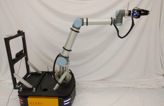
Figure 2: The UR10 industrial manipulator used in the experiments.

VII-A Experimental Setup

The interface to the UR10 does not permit direct torque control. Instead, only position and velocity control of the joints are available. Thus, for our proposed approach, we need to implement only the GP regression models and the robust, outer-loop controller. The commanded acceleration $a_{q}$ calculated by the outer-loop controller in (11) is integrated to obtain a velocity command that can be sent to the UR10. To test our approach for various uncertainties, we introduce artificial model uncertainty by adding a function $\eta(q,\dot{q},a_{q})$ to our calculated acceleration command $a_{q}$.

The PD gains of the outer-loop controller are tuned to achieve good tracking performance on a baseline desired trajectory in a nominal scenario with no added uncertainty. A desired trajectory of $q_{d}=0.25(1-\cos(2.0t))$ for each joint is used for this purpose, with gains selected to produce a total joint angle RMS error less than $0.01~{}\mathrm{rad}$. This resulted in $K_{p}=7.0I$ and $K_{d}=1.0I$, where $I$ is the identity matrix.

We use 6 GPs to learn the uncertainty vector $\eta$, each of which uses the squared exponential kernel. The prior variance and length scale hyperparameters are optimized by maximizing the marginal likelihood function, while each noise variance is set to $0.001$. Hyperparameter optimization is performed offline using approximately 1000 data points collected while tracking sinusoidal trajectories under uncertainty $\eta=0.5\dot{q}$. Implementation and tuning of the GPs are done with the Python library GPy. Each GP runs at $125~{}\mathrm{Hz}$, and uses the past $n=50$ observations for prediction. For the confidence intervals, we use $[\mu_{k}-3\sigma_{k},\mu_{k}+3\sigma_{k}]$ for simplicity [15]. For the robust controller, we use $\epsilon=0.1$.

VII-B Results

The performance of the proposed robust learning controller is initially compared to that of the nominal, outer-loop PD controller using a single trajectory and various cases of model uncertainty. Ten different cases of uncertainty of the form $\eta(q,\dot{q},a_{q})$ are tested over the desired trajectory $q_{d}=0.25(1-\cos(2.0t))$ for each joint, with the results displayed in Figure 3. The average RMS error of the nominal controller is $0.111~{}\mathrm{rad}$ and that of the proposed controller is $0.068~{}\mathrm{rad}$, yielding an average improvement of $41.5\%$.

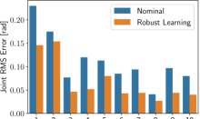
Figure 3: Joint RMS error of the nominal controller and the proposed robust learning controller for ten different uncertainties and a desired trajectory $q_{d}=0.25(1-\cos(2.0t))$ for each joint. The proposed method outperforms the nominal controller in all cases, with an average error reduction of $41.5\%$.

Further experiments were performed to verify the generalizability of the proposed approach for different desired trajectories that cover different regions of the state space. A single case of uncertainty, $\eta=0.3\dot{q}+0.01q\odot\dot{q}$ where $\odot$ is the entrywise product, is selected and the performance of the proposed and nominal controllers under this uncertainty is compared on five additional trajectories. The results are presented in Table II, with an average overall improvement of $39.9\%$ compared to the nominal controller. The six trajectories are shown in a demo video at http://tiny.cc/man-traj

TABLE II: RMS Tracking Error (in rad) for Various Trajectories with a Fixed Uncertainty Function $\eta=0.3\dot{q}+0.01q\odot\dot{q}$, where $\odot$ is the entrywise product

Trajectory	Nominal	Robust Learning	Improvement
1	0.070	0.037	47.1%
2	0.058	0.037	36.2%
3	0.092	0.058	37.0%
4	0.085	0.043	49.4%
5	0.050	0.029	42.0%
6	0.029	0.021	27.6%
Average	0.064	0.038	39.9%

To verify the reliability of the proposed method, experiments for six combinations of uncertainty and trajectory are repeated five times each with both the nominal and proposed robust learning controllers. The results are summarized in Figure 4. The figure shows that the performance under our proposed controller is highly repeatable and that it outperforms the nominal controller in all 30 cases.

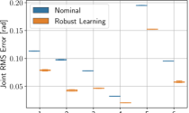
Figure 4: Box plots of six testing scenarios with different combinations of uncertainty and trajectory, each repeated five times. The bottom and top edges of each box show the 25^th and 75^th percentiles, respectively. The whiskers show the extreme values. The system performance is very repeatable, and our proposed controller outperforms the nominal controller in all cases (30 experiments in total).

VIII Conclusions

We have provided a novel, learning-based control strategy based on Gaussian processes (GPs) that ensures stability of the closed-loop system and high-accuracy tracking of smooth trajectories for an important class of Lagrangian systems. The main idea is to use GPs to estimate an upper bound on the uncertainty of the linearized model, and then use the uncertainty bound in a robust, outer-loop controller. Unlike most of the existing, learning-based inverse dynamics control techniques, we have provided a proof of the closed-loop stability of the system that takes into consideration the regression errors of the learning module. Moreover, we have proved that the tracking error converges to a ball with a radius that can be made arbitrarily small. Furthermore, we have verified the effectiveness of our approach via simulations on a planar manipulator and experimentally on a 6 DOF industrial manipulator.

References

- [1] M. W. Spong, S. Hutchinson, M. Vidyasagar. Robot Modeling and Control. John Wiley & Sons, Inc., 2006.
- [2] V. Hagenmeyer, E. Delaleau. Exact feedforward linearization based on differential flatness. International Journal of Control, 76(6), pp. 537-556, 2003.
- [3] C. Abdallah, D. M. Dawson, P. Dorato, M. Jamshidi. Survey of robust control for rigid robots. IEEE Control Systems Magazine, 11(2), pp. 24-30, 1991.
- [4] J. Sun de la Cruz. Learning Inverse Dynamics for Robot Manipulator Control. M.A.Sc. Thesis, University of Waterloo, 2011.
- [5] R. Calandra, S. Ivaldi, M. P. Deisenroth, E. Rueckert, J. Peters. Learning inverse dynamics models with contacts. IEEE International Conf. on Robotics and Automation, Seattle, 2015, pp. 3186-3191.
- [6] A. S. Polydoros, L. Nalpantidis, V. Kruger. Real-time deep learning of robotic manipulator inverse dynamics. IEEE/RSJ International Conf. on Intelligent Robots and Systems, Hamburg, 2015, pp. 3442-3448.
- [7] S. Zhou, M. K. Helwa, A. P. Schoellig. Design of deep neural networks as add-on blocks for improving impromptu trajectory tracking. IEEE Conf. on Decision and Control, Melbourne, 2017, pp. 5201-5207.
- [8] D. Nguyen-Tuong, J. Peters. Using model knowledge for learning inverse dynamics. IEEE International Conf. on Robotics and Automation, Anchorage, 2010, pp. 2677-2682.
- [9] J. F. Fisac, A. K. Akametalu, M. N. Zeilinger, S. Kaynama, J. Gillula, C. J. Tomlin. A general safety framework for learning-based control in uncertain robotic systems. arXiv preprint arXiv:1705.01292, 2017.
- [10] T. J. Perkins, A. G. Barto. Lyapunov design for safe reinforcement learning. The Journal of Machine Learning Research, 3, pp. 803-832, 2003.
- [11] J. W. Roberts, I. R. Manchester, R. Tedrake. Feedback controller parameterizations for reinforcement learning. IEEE Symposium on Adaptive Dynamic Programming and Reinforcement Learning, Paris, 2011, pp. 310-317.
- [12] P. Geibel, F. Wysotzki. Risk-sensitive reinforcement learning applied to control under constraints. Journal of Artificial Intelligence Research, 24, pp. 81-108, 2005.
- [13] M. Turchetta, F. Berkenkamp, A. Krause. Safe exploration in finite markov decision processes with Gaussian processes. Advances in Neural Information Processing Systems, Barcelona, 2016, pp. 4312-4320.
- [14] F. Berkenkamp, R. Moriconi, A. P. Schoellig, A. Krause. Safe learning of regions of attraction for uncertain, nonlinear systems with Gaussian processes. IEEE Conf. on Decision and Control, Las Vegas, 2016, pp. 4661-4666.
- [15] F. Berkenkamp, A. P. Schoellig, A. Krause. Safe controller optimization for quadrotors with Gaussian processes. IEEE International Conf. on Robotics and Automation, Stockholm, 2016, pp. 491-496.
- [16] G. Chowdhary, H. A. Kingravi, J. P. How, P. A. Vela. Bayesian nonparametric adaptive control using gaussian processes. IEEE trans. on neural networks and learning systems, 26(3), pp. 537-550, 2015.
- [17] F. Meier, D. Kappler, N. Ratliff, S. Schaal. Towards robust online inverse dynamics learning. IEEE/RSJ International Conf. on Intelligent Robots and Systems, Daejeon, 2016, pp. 4034-4039.
- [18] T. Beckers, J. Umlauft, D. Kulić, S. Hirche. Stable Gaussian process based tracking control of Lagrangian systems. IEEE Conf. on Decision and Control, Melbourne, 2017, pp. 5580-5585.
- [19] M. K. Helwa, A. P. Schoellig. On the construction of safe controllable regions for affine systems with applications to robotics. arXiv preprint arXiv:1610.01243, 2016.
- [20] R. M. Murray. Nonlinear control of mechanical systems: a Lagrangian perspective. Annual Reviews in Control, 21, pp. 31-42, 1997.
- [21] N. Srinivas, A. Krause, S. M. Kakade, M. W. Seeger. Information-theoretic regret bounds for Gaussian process optimization in the bandit setting. IEEE Trans. on Information Theory, 58(5), pp. 3250-3265, 2012.