The numerical algebraic geometry of bottlenecks

Abstract.

This is a computational study of bottlenecks on algebraic varieties. The bottlenecks of a smooth variety $X\subseteq\mathbb{C}^{n}$ are the lines in $\mathbb{C}^{n}$ which are normal to $X$ at two distinct points. The main result is a numerical homotopy that can be used to approximate all isolated bottlenecks. This homotopy has the optimal number of paths under certain genericity assumptions. In the process we prove bounds on the number of bottlenecks in terms of the Euclidean distance degree. Applications include the optimization problem of computing the distance between two real varieties. Also, computing bottlenecks may be seen as part of the problem of computing the reach of a smooth real variety and efficient methods to compute the reach are still to be developed. Relations to triangulation of real varieties and meshing algorithms used in computer graphics are discussed in the paper. The resulting algorithms have been implemented with Bertini [4] and Macaulay2 [17].

1. Introduction

Let $X,Y\subseteq\mathbb{C}^{n}$ be smooth varieties. For $x\in X$ and $y\in Y$ let $N_{x}X\subseteq\mathbb{C}^{n}$ and $N_{y}Y\subseteq\mathbb{C}^{n}$ denote the normal spaces at $x$ and $y$. Consider the incidence correspondence

$$I(X,Y)=\{(x,y)\in X\times Y:y\in N_{x}X,\;x\in N_{y}Y\}.$$

The goal is to set up an optimal numerical homotopy for the purpose of approximating the isolated points of $I(X,Y)$ given equations defining $X$ and $Y$ as well as the dimensions of $X$ and $Y$. In this context optimality means that the number of homotopy paths is equal to the number of solutions. In the sequel the isolated points of $I(X,Y)$ will be denoted $I(X,Y)_{0}$.

The main idea behind the homotopy is to first solve the following two initial problems for general points $p,q\in\mathbb{C}^{n}$:

$$\begin{array}[]{cc}\Sigma_{1}=\{x\in X:p\in N_{x}X\},&\Sigma_{2}=\{y\in Y:q\in N_{y}Y\}.\end{array}$$

The set of start points for the homotopy is essentially the product set $\Sigma_{1}\times\Sigma_{2}$. The system is then deformed so that $p$ approaches $y$ and $q$ approaches $x$, which yields points on the incidence set $I(X,Y)$. One may, as we do below, let $p=q$.

For $(x,y)\in I(X,Y)$ with $x\neq y$ the line joining $x$ and $y$ is normal to $X$ at $x$ and $Y$ at $y$. We will refer to these as bottlenecks. These lines correspond to the nontrivial critical points of the squared Euclidean distance function $\sum_{i=1}^{n}(x_{i}-y_{i})^{2}$, nontrivial meaning that $x\neq y$. Now, if $Y=\{p\}$ is just a point, this reduces to a type of polar variety which will be called the normal locus of $X$ with respect to $p$: $\{x\in X:p\in N_{x}X\}$. The normal class, which is the cohomology class of the normal locus for a general $p\in\mathbb{C}^{n}$, has been studied in [14, 23] where its degree is called the Euclidean distance degree. See also [18] for a relation to the problem of finding real points on algebraic varieties.

In Section 1.1 we describe some applications of bottlenecks to real geometry. Section 2 and Section 3 contain background material on numerical homotopy methods and the Euclidean distance degree. In Theorem 3.7 we show that optimality holds for the homotopy if $I(X,Y)$ is smooth and finite and $X$ and $Y$ satisfy some additional genericity assumptions. This means that under these assumptions, $I(X,Y)$ is the product of the Euclidean distance degrees of $X$ and $Y$. The homotopy itself is formulated in Section 4 and in Theorem 4.2 we prove that the isolated points of $I(X,Y)$ are included among the end points of the homotopy. In the process we prove bounds on the number of bottlenecks in terms of the Euclidean distance degrees of $X$ and $Y$, see Corollary 4.3 and Corollary 4.5. In Section 5 we briefly consider a variant of the problem where $X$ and $Y$ are projected to a lower dimensional affine space. The motivation for this is the usefulness of dimensionality reduction in various applications. In Section 6 and Section 7 we give some illustrative examples and compare the method to a more naive approach to solve the problem.

1.1. Applications to real geometry

Let $X,Y\subseteq\mathbb{R}^{n}$ be real algebraic sets and suppose that the complexifications $X_{\mathbb{C}}$ and $Y_{\mathbb{C}}$ are smooth complex varieties. The real points of the Euclidean normal space $N_{x}X_{\mathbb{C}}$ at a real point $x\in X$ is equal to the standard normal space of the real submanifold $X\subseteq\mathbb{R}^{n}$. The method presented in this paper may be applied to the problem of computing the distance between $X$ and $Y$. If we let $I(X,Y)$ be defined the same way as for complex varieties, we have that $I(X,Y)$ consists of the real points of $I(X_{\mathbb{C}},Y_{\mathbb{C}})$. If there is a point $(x,y)\in X\times Y$ realizing the infimum of the distance between points of $X$ and $Y$, for example if $X$ or $Y$ is compact, then $(x,y)\in I(X,Y)$. The same is true of the maximal distance if $X$ and $Y$ are compact. Considering the case $X=Y$, the method may also be applied to compute a lower bound for the distance between connected components of $X$. As above, if there is a point $(x,y)\in X\times X$ that realizes the minimal distance between points of any two different connected components of $X$, for example if $X$ is compact and not connected, then $(x,y)\in I(X,X)$.

The special case $X=Y$ is of particular interest. The meaning of the isolated points of $I(X,X)$ relates to the condition number or reach of $X$. This is roughly speaking the maximal size of an $\epsilon$-neighborhood of $X$ that embeds smoothly in $\mathbb{R}^{n}$. More precisely, the reach of $X$ is the supremum of the set of numbers $r\geq 0$ such that all points in $\mathbb{R}^{n}$ at distance less than $r$ from $X$ has a unique closest point on $X$. Assume that $X$ is compact and $\operatorname{dim}(X)>0$, in which case it has positive and finite reach. The reach is an important invariant for methods that seek to build a model of $X$ by covering it with balls of the ambient space $\mathbb{R}^{n}$ and forming the C̆ech complex or Vietoris-Rips complex corresponding to the balls. This has been proposed as a method to compute the homology of $X$ [22], see also the papers [10, 15, 19] on persistent homology in algebraic geometry. More generally, triangulation, meshing and similar procedures are important problems in computer graphics among other disciplines [2, 7, 8, 9, 12]. The reach is typically part of the input to algorithms proposed to solve such problems. Let $\rho$ be the minimal radius of curvature on $X$, where the radius of curvature at a point $x\in X$ is the reciprocal of the maximal curvature of a geodesic passing through $x$. Also, note that $I(X_{\mathbb{C}},X_{\mathbb{C}})$ contains $X_{\mathbb{C}}$ as an excess component in the form of $X_{\mathbb{C}}\times X_{\mathbb{C}}$ intersected with the diagonal of $\mathbb{C}^{n}\times\mathbb{C}^{n}$. The reach can be calculated in two stages, it is the minimum of $\rho$ and $\frac{1}{2}\inf\{||x-y||:(x,y)\in I(X,X)\setminus X\}$, see [1]. If $I(X_{\mathbb{C}},X_{\mathbb{C}})\setminus X_{\mathbb{C}}$ is finite and $X_{\mathbb{C}}$ satisfies the genericity conditions explained in Section 3, the latter infimum is a minimum which may be computed effectively using the homotopy presented in this paper.

1.2. Related work and future developments

There are some similarities between the method presented in this paper and the $\mathbb{C}^{*}$-action homotopy explored in the [13] but that homotopy involves higher powers of the path variable which is not the case for the homotopy described below. Based on numerical experiments this seems to be of importance in practice even though we have not carried out any such complexity analysis. Also, the intersection method presented in [24] is closely related to the present work.

As we are interested in applications to real geometry and the number of real solutions to the problem is sometimes much smaller than the number of complex solutions, it is worth considering a similar approach to compute the real solutions directly. For example one may approach this problem via real path tracking [6].

We have chosen to consider the Euclidean normal bundles of $X$ and $Y$ for the sake of applications to real geometry. However, the same technique is applicable for more general vector bundles on $X$ and $Y$ which should make possible other interesting applications.

2. Numerical homotopies for isolated roots

In this section we give a brief summary of numerical homotopy methods, see [5, 25] for details. These methods can be used to numerically find solutions to polynomial systems. Moreover it is possible to guarantee that all isolated solutions of the given system have been found. In homotopy methods we set up a deformation from a start system to the target system, which is the system that we would like to solve. The start system typically has known solutions and the idea is to track these points using a numerical predictor/corrector method to solutions of the target system.

More in detail, consider $m$ polynomials $H=\{H_{1},\dots,H_{m}\}\subset\mathbb{C}[x_{1},\dots,x_{m},t]$. Let $\mathcal{X}\subseteq\mathbb{C}^{m}\times\mathbb{C}$ be the subscheme defined by the ideal $(H_{1},\dots,H_{m})$ and let $\pi:\mathcal{X}\rightarrow\mathbb{C}$ be the projection. Suppose that we are interested in $X=\pi^{-1}(0)$, for instance we might want to approximate the isolated points of $X$. An example of this situation is that we are given $m$ polynomials $\{F_{1},\dots,F_{m}\}$ which define $X$ and let $H_{i}=F_{i}+tG_{i}$ for sufficiently general $G_{i}\in\mathbb{C}[x_{1},\dots,x_{m}]$ with $\operatorname{deg}(F_{i})=\operatorname{deg}(G_{i})$.

Homotopy methods can be used to approximate isolated points of $X$ by first approximating the isolated points of another fiber, say $\pi^{-1}(1)$. Suppose for simplicity that $\pi^{-1}(1)$ is smooth and finite. We then choose a path $\alpha:[0,1]\rightarrow\mathbb{C}$ with $\alpha(1)=1$ and $\alpha(0)=0$ and track the so-called solution paths. The solution paths are maps $\beta:(0,1]\rightarrow\mathcal{X}$ which satisfy $\pi\circ\beta=\alpha$ and there is one for each isolated point of $\pi^{-1}(1)$, provided that $\alpha$ is general enough as to avoid a finite number of points in $\mathbb{C}$. After projection to $\mathbb{C}^{m}$ a solution path may also be viewed as a map $(0,1]\rightarrow\mathbb{C}^{m}$, a perspective we will employ in the sequel. The solution paths satisfy an ODE known as the Davidenko equation and they can be tracked using an ODE solver. The isolated points of $\pi^{-1}(1)$ are known as start points in this context and they are the initial values for the ODE. If $\beta$ is a solution path that converges, the limit point is called the end point of the path. The tracking is simplest in the case of non-singular paths, that is when the Jacobian of $H$ with respect to $\{x_{1},\dots,x_{m}\}$ has full rank at all points of the path, including the end point if the path is convergent. The end point is in this case a smooth isolated point of $X$. The next simplest case is a convergent solution path which is non-singular except at the end point; such a path may converge to a multiple isolated point of $X$ or a higher dimensional component of $X$. To track such paths, or even paths of higher multiplicity, one may employ special techniques which are described in detail in [25].

In order to guarantee that all the isolated points of $X$ are among the end points of solution paths of the homotopy, we must have some control over the root count. This is the case for example if $\pi^{-1}(1)$ is smooth and finite, $\pi^{-1}(t)$ is smooth and finite for general $t\in\mathbb{C}$ and in addition $|\pi^{-1}(1)|=|\pi^{-1}(t)|$ for general $t\in\mathbb{C}$. This is the type of situation that we will encounter in this paper. Note that even if $\pi^{-1}(t)$ is smooth and finite for some $t\in\mathbb{C}$, the corresponding subscheme of $\mathbb{P}^{m}$ defined by homogenizing the system $H$ might have some nasty components at infinity, possibly of higher dimension. This in effect reduces the root count in $\mathbb{C}^{m}$ in the light of Bézout’s theorem and Fulton’s excess intersection formula [16] and this can be taken advantage of to set up more efficient homotopies with fewer paths to follow than the Bézout number would suggest. More generally we may consider only solutions contained in an open subset $U\subseteq\mathbb{P}^{m}$ and use this to reduce the number of homotopy paths. We will do this in connection with over determined systems in Section 4.2 and Section 4.3.

In order for it to make sense to use a homotopy to solve the problem, $\pi^{-1}(1)$ should be better understood or easier to handle somehow than $\pi^{-1}(0)$. One may for example set up the homotopy $H$ in such a way that $\pi^{-1}(1)$ has known isolated points. For the homotopy studied in this paper the start point computation is not trivial but of lower order complexity compared to the main problem of approximating the isolated points of $\pi^{-1}(0)$, see Theorem 3.7 and Corollary 4.3.

Numerical homotopies often depend on parameters in such a way that only a generic choice of these parameters yields a homotopy with desired properties. In practice one uses random parameters which results in probabilistic algorithms but since a general choice suffices it is often said that the desired properties hold with probability 1. Let $S^{1}\subset\mathbb{C}$ be the unit circle. The homotopy presented in this paper depends on two parameters $p_{0}\in\mathbb{C}^{n}$ and $\gamma\in S^{1}$ as well as the squaring of the systems for $X$ and $Y$ explained in Section 4.2. These parameters will be assumed to be general, and in practice they are taken as random vectors or matrices with complex entries.

3. Euclidean distance degree and bottlenecks

Let $X,Y\subseteq\mathbb{C}^{n}$ be smooth subvarieties and consider the closures $\bar{X},\bar{Y}\subseteq\mathbb{P}^{n}$. The hyperplane at infinity $H_{\infty}$ intersects $\bar{X}$ and $\bar{Y}$ in two subschemes $X_{\infty}=\bar{X}\cap H_{\infty}$ and $Y_{\infty}=\bar{Y}\cap H_{\infty}$. For a projective variety $Z\subseteq\mathbb{P}^{m}$, we use $\hat{Z}\subseteq\mathbb{C}^{m+1}$ to denote the cone over $Z$.

The smooth quadric $Q_{\infty}\subset H_{\infty}$ defined by $x_{1}^{2}+\dots+x_{n}^{2}=0$ is known as the isotropic quadric in $\mathbb{P}^{n-1}$. This choice of quadric induces a bilinear form on $\mathbb{C}^{n}$ as well as an orthogonality relation: for $x,y\in\mathbb{C}^{n}$ the condition $x\perp y$ is equivalent to $x^{T}y=0$ where $x$ and $y$ are viewed as column vectors. This is the definition of orthogonality we are using for our bottleneck problem. For a smooth variety $X\subseteq\mathbb{C}^{n}$ we will write $(T_{x}X)^{\perp}$ for the orthogonal complement of the embedded tangent space $T_{x}X$ translated to the origin. Similarly $z\perp T_{x}X$ for $z\in\mathbb{C}^{n}$ means that $z$ is orthogonal to $T_{x}X$ translated to the origin. The normal space at a point $x\in X$ is by definition $(T_{x}X)^{\perp}$ translated to $x$. For a general point $p_{0}\in\mathbb{C}^{n}$, $\{x\in X:(x-p_{0})\perp T_{x}X\}$ is finite and the number of points does not depend on $p_{0}$. This number is called the Euclidean distance degree of $X$ and is denoted $\operatorname{\epsilon}(X)$. For $X\times Y\subseteq\mathbb{C}^{2n}$, we have that $\operatorname{\epsilon}(X\times Y)=\operatorname{\epsilon}(X)\operatorname{\epsilon}(Y)$.

At a point $x\in X$ lines in the normal space through $x$ are parameterized by $\mathbb{P}^{n-d-1}$ where $d=\operatorname{dim}(X)$. There is an induced map $\Phi:X\times\mathbb{P}^{n-d-1}\rightarrow\operatorname{\mathbb{G}}(2,n+1)$ to the Grassmannian of lines in $\mathbb{P}^{n}$ which maps a line in $\mathbb{C}^{n}$ to its closure in $\mathbb{P}^{n}$. Similarly there is a map $\Gamma:Y\times\mathbb{P}^{n-e-1}\rightarrow\operatorname{\mathbb{G}}(2,n+1)$ where $e=\operatorname{dim}(Y)$ and a product map

$$\Phi\times\Gamma:X\times Y\times\mathbb{P}^{n-d-1}\times\mathbb{P}^{n-e-1}\rightarrow\operatorname{\mathbb{G}}(2,n+1)\times\operatorname{\mathbb{G}}(2,n+1).$$

Let $R=\pi((\Phi\times\Gamma)^{-1}(\Delta))$ where $\Delta\subset\operatorname{\mathbb{G}}(2,n+1)\times\operatorname{\mathbb{G}}(2,n+1)$ is the diagonal and $\pi$ is the projection to $X\times Y$. Note that there is an excess component of $I(X,Y)$ in the form of $X\cap Y$ written as $(X\times Y)\cap\Delta^{\prime}$ where $\Delta^{\prime}\subset\mathbb{C}^{n}\times\mathbb{C}^{n}$ is the diagonal and as sets $I(X,Y)=(X\cap Y)\cup R$. We expect that $\operatorname{dim}(\operatorname{im}(\Phi))=\operatorname{dim}(\operatorname{im}(\Gamma))=n-1$ and since $\operatorname{dim}(\operatorname{\mathbb{G}}(2,n+1))=2(n-1)$ we expect that $\operatorname{dim}(R)=0$.

Example 3.1.

Let $Q\subset\mathbb{P}^{2}$ be the isotropic quadric defined by $x_{0}^{2}+x_{1}^{2}+x_{2}^{2}=0$ and let $p\in Q$. Let $a,b\in l$ be general points on the tangent line $l$ to $Q$ at $p$. Now consider lines $X,Y\subset\mathbb{C}^{3}$ passing through $a$ respectively $b$ at infinity, but otherwise general. We may assume that $X$ and $Y$ are not coplanar. In this case $I(X,Y)=\emptyset$ and $\operatorname{\epsilon}(X)=\operatorname{\epsilon}(Y)=1$. To see that $I(X,Y)$ is empty, suppose that $(x,y)\in I(X,Y)$ and let $v,w\in\mathbb{C}^{3}$ represent the directions of $X$ and $Y$. Note that $v,w$ are homogeneous coordinates of the points $a,b\in\mathbb{P}^{2}$. Then $(x-y)\perp v,w$ and hence $(x-y)$ represents the line $l$ as well as the point $p\in\mathbb{P}^{2}$. This means that the closure $l^{\prime}\subset\mathbb{P}^{3}$ of the line joining $x$ and $y$ intersects the hyperplane at infinity at $p$ and the plane spanned by $l^{\prime}$ and $l$ contains both $X$ and $Y$, a contradiction.

As we saw in the last example, the bottleneck problem may have a kind of solutions at infinity which we are not interested in computing in the present context.

Definition 3.2.

Let $X,Y\subseteq\mathbb{C}^{n}$ be smooth varieties. If there is a pair of points $(x,y)\in\mathbb{C}^{n}\times\mathbb{C}^{n}$, with $x,y\neq 0$, $(x,y)\in\hat{X}_{\infty}\times\hat{Y}_{\infty}$, $(x-y)\perp T_{x}\hat{X}_{\infty}$ and $(x-y)\perp T_{y}\hat{Y}_{\infty}$ we will call the pair a solution at infinity to the bottleneck problem.

Example 3.3.

Let $A,B\subseteq\mathbb{P}^{n-1}$ be smooth algebraic sets, possibly reducible, and consider the cones $X=\hat{A}\setminus\{0\}$ and $Y=\hat{B}\setminus\{0\}$. We can define the incidence $I(X,Y)$ and the maps $\Phi$ and $\Gamma$ the same way as for varieties. In this case, the residual set $R$ above is a cone in the sense that $(tx,ty)\in R$ for all $(x,y)\in R$ and $t\in\mathbb{C}^{*}$. However, if we restrict $\Phi$ to $W=(X\cap H)\times\mathbb{P}^{n-d-1}$ where $H\subset\mathbb{C}^{n}$ is a general hyperplane, we have that $\operatorname{dim}(\operatorname{im}(\Phi|_{W}))\leq n-2$ and we expect the images of $\Phi|_{W}$ and $\Gamma$ to be disjoint. We thus expect the residual $R$ to be empty for cones. In particular we can expect the bottleneck problem of two smooth varieties $X,Y\subseteq\mathbb{C}^{n}$ to have no solutions at infinity beyond $\hat{X}_{\infty}\cap\hat{Y}_{\infty}$. See Example 3.1 for a pair of varieties in special position where this is not the case.

We now define the ED-correspondence

$$\mathcal{E}_{X\times Y}=\{(x,y,p,q)\in\mathbb{C}^{4n}:(x,y)\in X\times Y,\;(x-p)\perp T_{x}X,\;(y-q)\perp T_{y}Y\},$$

with its induced reduced structure. In [14] the ideal defining $\mathcal{E}_{X\times Y}$ is given and it is shown in Theorem 4.1 that it is an irreducible variety of dimension $2n$. If there is a point $(x,y)\in X\times Y$ such that $T_{x}X\cap N_{x}X=\{x\}$ and $T_{y}Y\cap N_{y}Y=\{y\}$, the projection $\mathcal{E}_{X\times Y}\rightarrow\mathbb{C}^{2n}:(x,y,p,q)\mapsto(p,q)$ is dominant and the generic fiber has $\operatorname{\epsilon}(X)\operatorname{\epsilon}(Y)$ points, see [14] Theorem 4.1. On the other hand, the projection is dominant if and only if $\operatorname{\epsilon}(X)$ and $\operatorname{\epsilon}(Y)$ are both non-zero.

Example 3.4.

Let $X\subset\mathbb{C}^{2}$ be the line defined by $x-iy$ where $i^{2}=-1$. Note that $X=T_{x}X=(T_{x}X)^{\perp}$ for every $x\in X$. Therefore $\operatorname{\epsilon}(X)=0$. The same is true for any cone over a subvariety of the isotropic quadric $\{x_{1}^{2}+\dots+x_{n}^{2}=0\}$ in $\mathbb{P}^{n-1}$.

We will frequently make the following assumptions on smooth varieties $X,Y\subseteq\mathbb{C}^{n}$:

(1) $$\operatorname{\epsilon}(X) \operatorname{\epsilon}(Y) X_{\infty} Y_{\infty} Q_{\infty}$$, are non-zero and , are smooth and intersect transversely.

Introduce a new variable $u$ and consider the closure $N=\bar{\mathcal{E}}_{X\times Y}\subset\mathbb{P}^{4n}$ and its intersection $N_{\infty}$ with the hyperplane at infinity given by $u=0$. For $p_{0}\in\mathbb{C}^{n}$, let $V_{s}(p_{0})$ for $s\in\mathbb{C}$ be the family of $2n$-dimensional linear spaces in $\mathbb{C}^{4n}$ defined by $p=(1-s)y+sp_{0}$, $q=(1-s)x+sp_{0}$.

Lemma 3.5.

Let $X,Y$ be as in (1) and let $N\subseteq\mathbb{P}^{4n}$ be the closure of the ED-correspondence. Let $p_{0}\in\mathbb{C}^{n}$ be generic.

1. $\operatorname{deg}(N)=\operatorname{\epsilon}(X)\operatorname{\epsilon}(Y)$,

2. the intersection $J_{s}=\mathcal{E}_{X\times Y}\cap V_{s}(p_{0})$ is transversal for generic $s\in\mathbb{C}$ and for $s=1$,

3. $|J_{1}|=|J_{s}|=\operatorname{\epsilon}(X)\operatorname{\epsilon}(Y)$ for generic $s\in\mathbb{C}$,

4. if the bottleneck problem of $X,Y$ has no solutions at infinity, then $N_{\infty}\cap\{x-q=y-p=0\}=\emptyset$.

Proof.

Let $(x,y,p,q,0)\in N_{\infty}$. We first show the following:

(2) If $$x\neq 0 x\in\hat{X}_{\infty} (x-p)\perp T_{x}\hat{X}_{\infty} y\neq 0 y\in\hat{Y}_{\infty} (y-q)\perp T_{y}\hat{Y}_{\infty}$$ then and . If then and .

Suppose that $x\neq 0$, the case $y\neq 0$ is similar. Let $(x_{i},y_{i},p_{i},q_{i},u_{i})\in\hat{N}\subseteq\mathbb{C}^{4n+1}$ for $i\in\mathbb{N}$ be a sequence such that $x_{i}\rightarrow x$, $p_{i}\rightarrow p$ and $u_{i}\rightarrow 0$ but $u_{i}\neq 0$ for all $i$. Then $x_{i}/u_{i}\in X$ and $(x_{i}/u_{i}-p_{i}/u_{i})\perp T_{x_{i}/u_{i}}X$ for all $i$. Hence $x\in\hat{X}_{\infty}$ and since $(x_{i}-p_{i})\perp T_{x_{i}/u_{i}}X$ for all $i$ it follows that $(x-p)\perp T_{x}\hat{X}_{\infty}$.

The intersection $J_{1}=\mathcal{E}_{X\times Y}\cap V_{1}(p_{0})$ is transversal, for example by generic smoothness and the fact that $p_{0}\in\mathbb{C}^{n}$ is generic. Clearly, $|J_{1}|=\operatorname{\epsilon}(X)\operatorname{\epsilon}(Y)$. Consider the linear space $\bar{V}_{1}(p_{0})=\{p-p_{0}u=q-p_{0}u=0\}\subset\mathbb{P}^{4n}$. If $(x,y,0,0,0)\in N_{\infty}\cap\bar{V}_{1}(p_{0})$, then either $x\neq 0$ or $y\neq 0$. Say that $x\neq 0$. Then, by (2), $x\perp T_{x}\hat{X}_{\infty}$ which contradicts that $X_{\infty}$ intersects the isotropic quadric $Q_{\infty}$ transversely. The same argument applies if $y\neq 0$. It follows that $N_{\infty}\cap\bar{V}_{1}(p_{0})=\emptyset$ and therefore $\operatorname{\epsilon}(X)\operatorname{\epsilon}(Y)=|J_{1}|=\operatorname{deg}(N)$. Moreover, it follows that $V_{s}(p_{0})$ intersects $\mathcal{E}_{X\times Y}$ transversely in $\operatorname{\epsilon}(X)\operatorname{\epsilon}(Y)$ points for generic $s\in\mathbb{C}$ as well.

It remains to show the last statement. Let $(x,y,p,q,0)\in N_{\infty}\cap\{x-q=y-p=0\}$. Then one of $x$ and $y$ is non-zero. If $y=0$ then $p=0$ and $x\perp T_{x}\hat{X}_{\infty}$ by (2). This contradicts that $X_{\infty}$ intersects the quadric $Q_{\infty}$ transversely. Hence $y\neq 0$ and similarly $x\neq 0$. Using (2) one more time we see that $x\in\hat{X}_{\infty}$, $y\in\hat{Y}_{\infty}$, $(x-y)\perp T_{x}\hat{X}_{\infty}$ and $(y-x)\perp T_{y}\hat{Y}_{\infty}$. Thus, $(x,y)$ represents a solution at infinity of the bottleneck problem. ∎

Let $V_{0}=\{x-q=y-p=0\}\subset\mathbb{C}^{4n}$ and note that the projection $\pi:\mathcal{E}_{X\times Y}\rightarrow X\times Y$ maps $V_{0}\cap\mathcal{E}_{X\times Y}$ bijectively onto $I(X,Y)$. This puts a scheme-structure on $I(X,Y)$ which we will use. Suppose that $X$ and $Y$ satisfy (1). If $I(X,Y)$ has multiple points or components of higher dimension, they contribute to the total multiplicity $\operatorname{\epsilon}(X)\operatorname{\epsilon}(Y)$ and makes $|I(X,Y)_{0}|$ smaller than this number. Since $(X\times Y)\cap\Delta^{\prime}\subseteq I(X,Y)$ where $\Delta^{\prime}\subset\mathbb{C}^{n}\times\mathbb{C}^{n}$ is the diagonal, $X\cap Y$ contributes to the total multiplicity and if $X$ and $Y$ intersect in higher dimension the number of isolated points of $I(X,Y)$ is smaller than $\operatorname{\epsilon}(X)\operatorname{\epsilon}(Y)$. The following example of varieties not satisfying (1) shows that $|I(X,Y)_{0}|$ can be bigger than $\operatorname{\epsilon}(X)\operatorname{\epsilon}(Y)$.

Example 3.6.

Let $X\subset\mathbb{C}^{3}$ be the line $ix_{1}-x_{2}=x_{3}=0$. In this case $\operatorname{\epsilon}(X)=0$ and the point $X_{\infty}$ lies on the quadric $Q_{\infty}\subset\mathbb{P}^{2}$. Note that $T_{x}X=X$ and $(T_{x}X)^{\perp}=N_{x}X=\langle X,(0,0,1)\rangle$ for all $x\in X$. Now let $Y\subset\mathbb{C}^{3}$ be a general line. The line $Y$ intersects $\langle X,(0,0,1)\rangle$ in exactly one point $y\in Y$ and the plane $N_{y}Y$ intersects $\langle X,(0,0,1)\rangle$ in a line which intersects $X$ in a point $x\in X$. Hence $I(X,Y)$ consists of one point $(x,y)$ but $\operatorname{\epsilon}(X)\operatorname{\epsilon}(Y)=0$.

The following theorem states that the homotopy presented in this paper is optimal if $X,Y$ satisfy (1), $I(X,Y)$ is finite and non-singular and the bottleneck problem has no solutions at infinity.

Theorem 3.7.

If $X,Y\subseteq\mathbb{C}^{n}$ are smooth varieties satisfying (1), $I(X,Y)$ is finite and non-singular and the bottleneck problem has no solutions at infinity, then

$$|I(X,Y)|=\operatorname{\epsilon}(X)\operatorname{\epsilon}(Y).$$

Proof.

Let $L=\{x-q=y-p=0\}\subset\mathbb{P}^{4n}$. We have assumed that the intersection $L\cap\mathcal{E}_{X\times Y}$ is transversal. By Lemma 3.5, $L\cap N_{\infty}=\emptyset$ and $|I(X,Y)|=\operatorname{deg}(N)=\operatorname{\epsilon}(X)\operatorname{\epsilon}(Y)$. ∎

3.1. Reformulation in terms of classical invariants

Let $X\subseteq\mathbb{C}^{n}$ be a smooth subvariety satisfying the assumptions (1). Then $\operatorname{\epsilon}(X)$ may be expressed in terms of the degrees $\mu_{i}(\bar{X})$ of the so-called polar classes of $\bar{X}$. In fact, as is shown in [14] Theorem 6.11,

$$\operatorname{\epsilon}(X)=\sum_{i=0}^{d}\mu_{i}(\bar{X}),$$

where $d=\operatorname{dim}(X)$. Since $\bar{X}$ is smooth, this may be expressed in terms of the degrees $c_{i}$ of the Chern classes of the tangent bundle of $\bar{X}$:

$$\operatorname{\epsilon}(X)=\sum_{i=0}^{d}(-1)^{i}\cdot(2^{d+1-i}-1)c_{i}.$$

See for example [16] Example 14.4.15 for the definition of polar classes and their relationship to Chern classes. As is explained in [23], another way to phrase this is in terms of the degree of the top Segre class of the Euclidean normal bundle: $\operatorname{\epsilon}(X)=\operatorname{deg}(s_{d}(N_{X}))$.

Example 3.8.

If $X\subseteq\mathbb{C}^{3}$ is a general surface of degree $d$, then $\operatorname{\epsilon}(X)=d^{3}-d^{2}+d$. Hence, if $X,Y\subseteq\mathbb{C}^{3}$ are general surfaces of degree $d$ and $e$,

$$|I(X,Y)_{0}|=(d^{3}-d^{2}+d)(e^{3}-e^{2}+e)-c,$$

where $c$ is the contribution from $X\cap Y$. Based on experiments, it seems that $c=de(d+e-1)$.

4. The homotopy

In this section we present the homotopy. As mentioned in the introduction, the start points of the homotopy are built from combining points in the normal loci of $X$ and $Y$ with respect to a general point $p_{0}\in\mathbb{C}^{n}$. This will be explained in detail below but for now let $p_{0}\in\mathbb{C}^{n}$ be a general point.

Suppose that $X\subset\mathbb{C}^{n}$ is a smooth variety defined by an ideal $(F_{1},\dots,F_{a})\subseteq\mathbb{C}[x_{1},\dots,x_{n}]$ and that $Y\subset\mathbb{C}^{n}$ is a smooth variety defined by $(G_{1},\dots,G_{b})$. For the sake of presentation, assume for now that $X$ and $Y$ are complete intersections and that $a=\operatorname{codim}(X)$ and $b=\operatorname{codim}(Y)$. The general case will be addressed below. Note that the set of lines in a fiber $N_{x}X$ that pass through the base point $x\in X$ may be viewed as $\mathbb{P}^{a-1}$. There is a map $X\times\mathbb{P}^{a-1}\rightarrow\mathbb{P}^{n-1}$ which sends $(x,l)$, where $x\in X$ and $l$ is a line in $N_{x}X$ through $x$, to the direction of $l$. Similarly there is a corresponding map $Y\times\mathbb{P}^{b-1}\rightarrow\mathbb{P}^{n-1}$ for $Y$. We will express these maps using the defining equations as follows. Let $J_{F}$ and $J_{G}$ be the Jacobian matrices of $F=(F_{1},\dots,F_{a})$ and $G=(G_{1},\dots,G_{b})$. Then, the normal line maps described above are induced by the maps $f:X\times\mathbb{C}^{a}\rightarrow\mathbb{C}^{n}:(x,v)\mapsto J_{F}(x)^{T}v$ and $g:Y\times\mathbb{C}^{b}\rightarrow\mathbb{C}^{n}:(y,w)\mapsto J_{G}(y)^{T}w$. The homotopy is given by the following equations:

(3) $$\begin{array}[]{c}F(x)=0,\\ G(y)=0,\\ s(x-p_{0})+(1-s)(x-y)-f(x,v)=0,\\ s(y-p_{0})+(1-s)(y-x)-g(y,w)=0,\end{array}$$

for $(x,y,v,w,s)\in\mathbb{C}^{n}\times\mathbb{C}^{n}\times\mathbb{C}^{a}\times\mathbb{C}^{b}\times\mathbb{C}$.

To define the path $\alpha:[0,1]\rightarrow\mathbb{C}$ described in Section 2 we introduce a general parameter $\gamma\in S^{1}\subset\mathbb{C}$ and use what in [25] is called the gamma trick. Based on the gamma trick we may use the path $\alpha:[0,1]\rightarrow\mathbb{C}$, $\alpha(t)=\gamma t/(1+(\gamma-1)t)$, which for a general $\gamma\in S^{1}$ ensures sufficient generality and avoids degeneracy. Letting $s=\alpha(t)$ in (3) we get

(4) $$\begin{array}[]{c}F(x)=0,\\ G(y)=0,\\ \gamma t(x-p_{0})+(1-t)(x-y)-(\gamma t+1-t)\cdot f(x,v)=0,\\ \gamma t(y-p_{0})+(1-t)(y-x)-(\gamma t+1-t)\cdot g(y,w)=0,\end{array}$$

for $(x,y,v,w,t)\in\mathbb{C}^{n}\times\mathbb{C}^{n}\times\mathbb{C}^{a}\times\mathbb{C}^{b}\times[0,1]$.

Remark 4.1.

Note that (4) with $t=0$ is the system we get if we apply Lagrange multipliers in the real setting to solve the optimization problem of minimizing or maximizing $||x-y||^{2}$ under the constraints $F(x)=G(y)=0$. We will compare our approach to more direct ways of solving this system in Section 7.

4.1. Equations for the start system

A system of equations for the start points with respect to a point $p_{0}\in\mathbb{C}^{n}$ is given by

$$F(x)=0,\;(x-p_{0})=f(x,v),$$

in the case of $X$ and similarly for $Y$. These equations may be homogenized with respect to the variables $v\in\mathbb{C}^{a}$ to yield a system homogeneous and linear in the these variables. The start points are $S_{1}\times S_{2}$ where

(5) $$\begin{array}[]{l}S_{1}=\{(x,v)\in X\times\mathbb{C}^{a}:(x-p_{0})=f(x,v)\}\\ S_{2}=\{(y,w)\in Y\times\mathbb{C}^{b}:(y-p_{0})=g(y,w)\}.\end{array}$$

Since we have ordered the coordinates of the homotopy as $(x,y,v,w)$, this has to be read as $S_{1}\times S_{2}=\{(x,y,v,w):(x,v)\in S_{1},\;(y,w)\in S_{2}\}$.

4.2. Effects of squaring the system

If $X$ is defined by more than $a=\operatorname{codim}(X)$ equations we need to square the system which we do by replacing defining equations $(\hat{F}_{1},\dots,\hat{F}_{r})$ for $X$ by $a$ general linear combinations $F=(F_{1},\dots,F_{a})$ of $(\hat{F}_{1},\dots,\hat{F}_{r})$. Similarly, given defining equations $(\hat{G}_{1},\dots,\hat{G}_{s})$ for $Y$ such that $s>b=\operatorname{codim}(Y)$, these are replaced by $b$ general linear combinations $G=(G_{1},\dots,G_{b})$ of $(\hat{G}_{1},\dots,\hat{G}_{s})$. The homotopy is then given by (4) applied to the systems $F$ and $G$. In the case $X=Y$ defined by $(\hat{F}_{1},\dots,\hat{F}_{r})$ we may take $F=G$. This is convenient as there is no need to solve the start system twice in this case.

The squaring of the system has the effect that $F$ and $G$ define some subschemes $X^{\prime},Y^{\prime}\subseteq\mathbb{C}^{n}$ with $X\subseteq X^{\prime}$ and $Y\subseteq Y^{\prime}$. Suppose that $X,Y\neq\emptyset$. By Bertini’s theorem, $X^{\prime}\times Y^{\prime}$ is equidimensional of dimension $\operatorname{dim}(X)+\operatorname{dim}(Y)$ and $X\times Y$ is an irreducible component of $X^{\prime}\times Y^{\prime}$. Let $\Sigma_{1}=\{x\in X:p_{0}\in N_{x}X\}$ and $\Sigma_{2}=\{y\in Y:p_{0}\in N_{y}Y\}$. We may assume that the finite subsets $\Sigma_{1}\times\Sigma_{2}$ and $I(X,Y)_{0}$ of $X\times Y$ are inside the smooth locus of $X^{\prime}\times Y^{\prime}$. It follows that $(\Sigma_{1}\times\Sigma_{2})\cap W=I(X,Y)_{0}\cap W=\emptyset$ for any irreducible component $W\subseteq X^{\prime}\times Y^{\prime}$ other than $X\times Y$. In particular, this means that every isolated point of $I(X,Y)$ lifts to an isolated solution of the squared system (3) over $s=0$.

Considering the equations for the start system in the general case of over determined systems, we can still use the equations given by $F(x),(x-p_{0})-f(x,v)$ and $G(y),(y-p_{0})-g(y,w)$ described in Section 4.1. However, we must pick only points $(x,y,v,w)\in X\times Y\times\mathbb{C}^{a}\times\mathbb{C}^{b}$ as in (5). Since the equations defining $X$ and $Y$ are part of the input, this can be done by a simple filtering process by evaluating the defining equations on tentative start points. One may also solve a corresponding over determined system with standard homotopy methods. Either way, the since start point computation is of lower order complexity it is not the focus of this paper.

4.3. Isolated points of the bottleneck problem

Let $S_{1}$ and $S_{2}$ be as in (5). Then $|S_{1}|=\operatorname{\epsilon}(X)$ and $|S_{2}|=\operatorname{\epsilon}(Y)$. Hence the number of start points $S_{1}\times S_{2}$ is $\operatorname{\epsilon}(X)\operatorname{\epsilon}(Y)$.

Theorem 4.2.

Let $X,Y\subset\mathbb{C}^{n}$ be smooth subvarieties that satisfy (1). The homotopy (4) has $\operatorname{\epsilon}(X)\operatorname{\epsilon}(Y)$ solution paths starting at $S_{1}\times S_{2}$ whose endpoints after projection to $\mathbb{C}^{2n}$ include all the isolated points of $I(X,Y)$. The paths are non-singular except possibly at the end points.

Proof.

Using the notation of Section 4.2, $X\times Y$ is a component of the subscheme $X^{\prime}\times Y^{\prime}\subset\mathbb{C}^{n}\times\mathbb{C}^{n}$ defined by the system $(F,G)$. Let $U_{0}=\mathbb{C}^{n}\times\mathbb{C}^{n}\setminus\overline{X^{\prime}\times Y^{\prime}\setminus X\times Y}$ and $U=U_{0}\times\mathbb{C}^{a+b}$. By Section 4.2, we may assume that the isolated points of $I(X,Y)$ are contained in $U_{0}$ and that $S_{1}\times S_{2}\subset U$. For $s=1$, the set of solutions to (3) contained in $U$ is equal to $S_{1}\times S_{2}$ and those solutions are smooth. Since $|S_{1}\times S_{2}|=\operatorname{\epsilon}(X)\operatorname{\epsilon}(Y)$, we have to show that for general $s\in\mathbb{C}$, the number of solutions to (3) contained in $U$ is equal to $\operatorname{\epsilon}(X)\operatorname{\epsilon}(Y)$. Once this is established, the statement follows from the general theory of parameter homotopies, see for example [25] Theorem 7.1.6 together with the gamma trick [25] Lemma 7.1.3.

Using the notation of Section 3, let $\mathcal{E}_{X\times Y}$ be the ED-correspondence, $V_{s}(p_{0})$ the family of linear spaces defined there and let $\pi:\mathcal{E}_{X\times Y}\rightarrow\mathbb{C}^{n}\times\mathbb{C}^{n}$ be the projection $(x,y,p,q)\mapsto(x,y)$. For generic $s\in\mathbb{C}$, there is a one-to-one correspondence between the solutions to (3) contained in $U$ and $\mathcal{E}_{X\times Y}\cap V_{s}(p_{0})\cap\pi^{-1}(U_{0})$. It is given by the map $\mathbb{C}^{n}\times\mathbb{C}^{n}\times\mathbb{C}^{a}\times\mathbb{C}^{b}\rightarrow\mathbb{C}^{4n}$ defined by

$$(x,y,v,w)\mapsto\begin{pmatrix}x\\ y\\ (1-s)y+sp_{0}\\ (1-s)x+sp_{0}\end{pmatrix}.$$

Since $\mathcal{E}_{X\times Y}\cap V_{1}(p_{0})\subseteq\pi^{-1}(U_{0})$ we have that $\mathcal{E}_{X\times Y}\cap V_{s}(p_{0})\subseteq\pi^{-1}(U_{0})$ for generic $s\in\mathbb{C}$ as well. By Lemma 3.5, $|\mathcal{E}_{X\times Y}\cap V_{s}(p_{0})|$ is finite and equal to $\operatorname{\epsilon}(X)\operatorname{\epsilon}(Y)$ for generic $s\in\mathbb{C}$. ∎

Corollary 4.3.

Let $X,Y\subset\mathbb{C}^{n}$ be smooth varieties that satisfy (1). Then $|I(X,Y)_{0}|\leq\operatorname{\epsilon}(X)\operatorname{\epsilon}(Y)$.

Remark 4.4.

If $X=Y$ with $\operatorname{dim}(X)>0$ it is enough to form the start points from all pairs $(s_{1},s_{2})$ with $s_{1},s_{2}\in S_{1}=S_{2}$, $s_{1}\neq s_{2}$ and without taking the order into account. We can still generate all the isolated points of $I(X,X)$ from the end points of the solution paths using the action $(x,y)\mapsto(y,x)$ on $I(X,X)$. This is because the homotopy is in this case invariant under the symmetry $(x,y,v,w)\mapsto(y,x,w,v)$. Of course, $(x,y)\in I(X,X)$ and $(y,x)\in I(X,X)$ with $x\neq y$ represent the same bottleneck, which is what we are really interested in. Any start point that is fixed under the symmetry, that is it comes from a pair $(s_{1},s_{1})$ with $s_{1}=(x,v)\in S_{1}$, can be discarded as the corresponding solution path projected to $X\times X$ is constant with value $(x,x)$. But $(x,x)\in I(X,X)$ is not isolated, unless $X$ is a point.

Corollary 4.5.

Let $X\subset\mathbb{C}^{n}$ be a smooth variety that satisfies (1). Then the number of isolated bottlenecks to $X$ is bounded by ${\operatorname{\epsilon}(X)\choose 2}$.

5. Linear projections

In applications it is often relevant to consider smooth maps $\pi:\mathbb{C}^{n}\rightarrow\mathbb{C}^{m}$ where $m<n$ such that $\pi_{|X}$ and $\pi_{|Y}$ are embeddings of $X$ and $Y$ with smaller codimension. For example, algorithms in the spirit of marching cubes [12] are sensitive to the dimension of the ambient space $n$ and are typically exponential in $n$. For these reasons it is useful to have a formulation of the homotopy that computes the isolated points of $I(\pi(X),\pi(Y))$ rather than $I(X,Y)$. The assumption is that we have equations for $X$ and $Y$ and that the map $\pi$ is given although equations for $\pi(X)$ and $\pi(Y)$ might not be available. On $\mathbb{C}^{n}$ and $\mathbb{C}^{m}$ we have bilinear forms $\langle\cdot,\cdot\rangle$ induced by the standard scalar products on $\mathbb{R}^{n}$ and $\mathbb{R}^{m}$. For $x\in X$ consider the differential $d\pi_{x}:T_{x}\mathbb{C}^{n}\rightarrow T_{\pi(x)}\mathbb{C}^{m}$ which induces as isomorphism between the embedded tangent spaces $T_{x}X\rightarrow T_{\pi(x)}\pi(X)$, seen as subspaces of $T_{x}\mathbb{C}^{n}\cong\mathbb{C}^{n}$ and $T_{\pi(x)}\mathbb{C}^{m}\cong\mathbb{C}^{m}$. For $x\in X$, $p_{0}\in\mathbb{C}^{n}$ and $z\in T_{x}X$ we have that $\langle\pi(x)-\pi(p_{0}),d\pi_{x}(z)\rangle=\langle\operatorname{adj}(d\pi_{x})(\pi(x)-\pi(p_{0})),z\rangle$ where $\operatorname{adj}(d\pi_{x})$ is the adjoint map. To find the normal locus of $\pi(X)$ with respect to $\pi(p_{0})$ we may thus compute the set of points $x\in X$ such that $\operatorname{adj}(d\pi_{x})(\pi(x)-\pi(p_{0}))\perp T_{x}X$. In a similar fashion we get the equations of the main homotopy in this setting:

$$\begin{array}[]{c}F(x)=0,\\ G(y)=0,\\ \operatorname{adj}(d\pi_{x})[\gamma t(\pi(x)-\pi(p_{0}))+(1-t)(\pi(x)-\pi(y))]-(\gamma t+1-t)\cdot f(x,v)=0,\\ \operatorname{adj}(d\pi_{y})[\gamma t(\pi(y)-\pi(p_{0}))+(1-t)(\pi(y)-\pi(x))]-(\gamma t+1-t)\cdot g(y,w)=0.\end{array}$$

Now assume that $\pi:\mathbb{C}^{n}\rightarrow\mathbb{C}^{m}$ is a linear map whose restriction to $X$ and $Y$ are embeddings. In the case of a smooth variety $X=Y$, these assumptions are met by a general linear map $\mathbb{C}^{n}\rightarrow\mathbb{C}^{m}$ where $m=2\cdot\operatorname{dim}(X)+1$ and a simple way to reduce ambient dimension in practice in case $n>2\cdot\operatorname{dim}(X)+1$ is to use a random linear map. In Example 6.1 we will consider real curves in higher codimension and project these to $\mathbb{R}^{3}$ for visualization purposes. In the case where $\pi$ is linear and represented by an $m\times n$-matrix $M$, the homotopy above becomes:

$$\begin{array}[]{c}F(x)=0,\\ G(y)=0,\\ M^{T}M(\gamma t(x-p_{0})+(1-t)(x-y))-(\gamma t+1-t)\cdot f(x,v)=0,\\ M^{T}M(\gamma t(y-p_{0})+(1-t)(y-x))-(\gamma t+1-t)\cdot g(y,w)=0.\end{array}$$

6. Examples

For the implementation of the examples below we have used Bertini [4] and Macaulay2 [17] with the package [3]. The timings were done using a 2.8 GHz processor of type Intel i7-2640M. More elaborate timings are performed in Section 7. The plotting was done using Matplotlib [20].

Example 6.1.

Consider a complete intersection curve $X\subseteq\mathbb{R}^{n}$ defined by $n-2$ random polynomials of degree 2 in $\mathbb{R}[x_{1},\dots,x_{n}]$ and the a hyperellipsoid $\sum_{i=1}^{n}r_{i}x_{i}^{2}-1$ where $0\leq r_{1}\leq 1$ are random. The reason for including the hyperellipsoid is to ensure compactness of $X$. In addition to this we require that the random quadrics pass through a random point on the hyperellipsoid, this is to ensure that $X$ is not empty. The method to compute bottlenecks described above was performed with both input varieties equal to $X_{\mathbb{C}}$, with $X$ as above for $n=2$, $n=3$, $n=4$ and $n=7$. Figure 1 displays plots of some of the results. For visualization purposes we have performed the method subject to a random orthogonal projection to $\mathbb{R}^{3}$ in the cases $n>3$ as in Section 5. In the figure, the computed bottlenecks are represented by a pair of red points on $X$ together with the line segment that joins them. We have also sampled $X$ (blue points) to visualize the curve. Plots without the normal lines are also included.

To get a sense of the timing, in the case of $n=4$ the start point homotopy follows 32 paths and the main homotopy follows 496 paths. The computation takes 2-3 seconds in this case. In the case $n=7$ the start homotopy follows 448 paths and the main homotopy follows 100128 paths. The number of real bottlenecks can however be quite small, in the random example tested it was only 6. The computation takes 20-25 minutes in this case.

Figure 1. Plots of complete intersection curves.

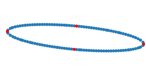
(a)

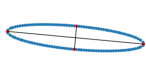
(b)

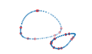
(c)

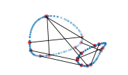
(d)

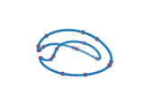
(e)

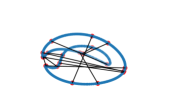
(f)

Example 6.1 in a sense exemplifies the worst case scenario as the start point homotopy for these random complete intersection curves is optimal and has as many paths as there are solutions to the start system (this follows from the discussion in Section 7, see also [14] Corollary 2.10). More benefit from the method is obtained in cases where structure is detected during the start system run, embodied in the fact that the start system has fewer solution than expected. This in turn means that fewer paths have to be followed for the main homotopy. This is illustrated in Section 7.

Example 6.2.

The method to compute bottlenecks was performed on the complexification of the Goursat surface in $\mathbb{R}^{3}$ defined by

$$x^{4}+y^{4}+z^{4}+(x^{2}+y^{2}+z^{2})^{2}-2(x^{2}+y^{2}+z^{2})-3=0.$$

The start point homotopy follows 108 paths and there are 52 solutions. This means that 1326 paths are followed by the main homotopy. There are 13 real bottlenecks which are plotted together with a sampling of the surface in Figure 2. In total the computation takes about 6 seconds.

Figure 2. A surface in $\mathbb{R}^{3}$.

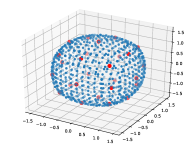
(a)

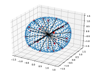
(b)

Example 6.3.

The following example originates from computational chemistry and explores the geometry of molecular conformation spaces. A cycloheptane molecule is a ring of seven coal atoms with a pair of hydrogen atoms bonded to each coal atom. Cycloheptane is a special case of a cycloalkane molecule and we will use a mechanical model of such molecules from the computational chemistry literature [21]. For the geometry of this model only the positions of the coal atoms in space are relevant. One way of viewing the model is to consider a conformation, or configuration, of the molecule as an embedding into $\mathbb{R}^{3}$ of the cycle-graph with 7 vertices, subject to constraints. The constraints are given by fixing the edge lengths, that is the distance between two consecutive atoms in the ring, as well as the angle between consecutive edges, that is the bond angles. In this model all the edge lengths are equal and all the bond angles are equal. We may set the edge lengths to 1 and the bond angle for this example was chosen to be 115 degrees, see [11] Chapter 25.2 for a discussion of bond angles of cycloalkane molecules.

The variety $X$ parameterizing conformations may be considered in $\mathbb{R}^{21}$ with three coordinates for each of the seven vertices of the graph. All in all we have seven distance constraints and seven angle constraints. In addition we are only interested in configurations up to rigid motion, that is up to the action of the six-dimensional special Euclidean group. We thus expect the variety of all conformations to be a curve, which it is. One way to deal with rigid motions is to fix three of the vertices in a way that is consistent with the distance and angle constraints. This way we get rid of nine variables and three of the constraints will be automatically satisfied. This gives us a curve in $\mathbb{R}^{12}$ defined by eleven polynomials. Moreover, two of the remaining angle constraints are now linear and it is therefore natural to consider the corresponding curve $X\subset\mathbb{R}^{10}$ defined nine quadratic polynomials.

One of the most basic questions about the geometry of $X$ is how many connected components it has. In this example, we apply the method for computing the isolated points of $I(X_{\mathbb{C}},X_{\mathbb{C}})$ to address this question.

In this context one may ask if the complexification $X_{\mathbb{C}}$ of $X$ satisfies the assumptions made throughout this paper. It is easy to verify with techniques from numerical algebraic geometry [4, 5, 25] that $X_{\mathbb{C}}$ is an irreducible curve of degree 112. Smoothness of $X_{\mathbb{C}}$ can be verified numerically as well, at least if done with some care. Instead of considering an ideal generated by minors of the Jacobian matrix $J$ it is better to introduce auxiliary variables $v=(v_{1},\dots,v_{10})$ and a random linear form $l(v)\in\mathbb{C}[v_{1},\dots,v_{10}]$ and express the rank condition on $J$ as nine bilinear equations $Jv^{T}=0$ together with $l(v)=0$. Alternatively, one may introduce variables $v=(v_{1},\dots,v_{9})$ and express the rank condition as $vJ=0$. Regarding the assumptions (1), the assumption that the Euclidean distance degree is positive is tested during the procedure. To avoid intersection with the isotropic quadric at infinity we make a random change of coordinates, that is we change coordinates using a real $10\times 10$-matrix. It is enough to use a random real diagonal matrix, which is preferable in order to preserve sparseness. One should be aware that changing coordinates by a non-orthogonal linear transformation does not in general respect bottlenecks but it does preserve the number of components of $X$. The assumption that $(X_{\mathbb{C}})_{\infty}$ is smooth in Lemma 3.5 is convenient but a bit stronger than necessary, it is enough that $X_{\mathbb{C}}$ is disjoint from the isotropic quadric at infinity. Finally, one may easily check numerically that $I(X_{\mathbb{C}},X_{\mathbb{C}})$ has no higher dimensional component except for $X_{\mathbb{C}}$. If that were the case, the normal space at a general point $x\in X_{\mathbb{C}}$ would intersect $X_{\mathbb{C}}$ in some point $y$ such that the line joining $x$ and $y$ is normal to $X_{\mathbb{C}}$ at $y$.

The homotopy (4) was run with both input varieties equal to $X_{\mathbb{C}}$ after changing coordinates as above. This gives us a lower bound for the distance between two connected components of $X$, namely $b=\min\{||x-y||:(x,y)\in(I(X_{\mathbb{C}},X_{\mathbb{C}})_{0})_{\mathbb{R}}\}$. To get a sense of the timing, the start point homotopy follows 5120 paths and there are 448 solutions. This means that the main homotopy follows 100128 paths. The whole computation takes about 2 h.

Now, given the lower bound $b$ on the distance between connected components it is straightforward to compute the number of components of $X$ with a sampling procedure and building the Vietoris-Rips complex with parameter $r<b/2$. Given a finite sample $E\subset X$ of $X$ this is simply the graph with vertex set $E$ and edges $\{(e_{1},e_{2})\in E\times E:0<||e_{1}-e_{2}||<2r\}$. The sampling can be done with standard homotopy methods. We will not go into details of this procedure in the present paper but the density of the sample has to be high enough, as measured with respect to the distance in the ambient space. Namely, we need to guarantee that given any point of $X$ there is a point of $E$ at distance less than $r$. It is straightforward to set up a sampling procedure that guarantees this by intersecting $X$ with a fine enough grid of hyperplanes in $\mathbb{R}^{10}$. This procedure was carried out and the result is that the curve $X$ has two connected components. Of course, several steps in this computation are subject to numerical errors, a subject we will not go into here (see [15] for a related discussion). Figure 3 shows the curve before the change of coordinates. The curve is drawn using so-called torsion angles (see [21]) as coordinates and a random orthogonal projection of these to $\mathbb{R}^{3}$.

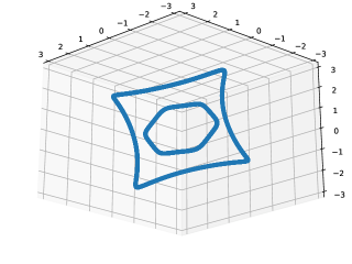
Figure 3. Cycloheptane conformation curve in torsion angles projected to $\mathbb{R}^{3}$.

7. Efficiency

The main complexity measure when comparing homotopy methods is the number of paths. We will compare our approach to solving (3) with $s=0$ using standard homotopies. For example one may use a total degree homotopy but since the system is linear in $v$ and $w$ the comparison was instead made to the more efficient formulation as a multihomogeneous homotopy over $\mathbb{C}^{2n}\times\mathbb{P}^{a}\times\mathbb{P}^{b}$. There are many alternatives to this, for example one may eliminate $x$ or $y$ from the equations (3) with $s=0$, which will decrease the number of variables but increase the degrees. Another alternative is to not use the auxiliary variables $v$ and $w$ at all and express the orthogonality conditions in terms of the vanishing of minors of matrices composed from the Jacobians $J_{F}$, $J_{G}$ and the vector $x-y$. If these reformulations are useful depends among other things on the codimension of $X$ and $Y$.

As a first example consider general surfaces $X,Y\subset\mathbb{C}^{3}$ of degree $d$. In this case we have that $|I(X,Y)_{0}|$ is equal to $(d^{3}-d^{2}+d)^{2}$ minus a contribution from $X\cap Y$ as in Example 3.8. Below we include random examples of this kind for some values of $d$, including one example where $X=Y$ and $X$ is random of degree 3.

The beneficial effects of the specialized homotopy are best seen when the invariants of $X$ and $Y$ are such that the number of solutions to the problem is small. This is gauged during the start point computations and fewer paths may be followed for the main homotopy in these cases. For example, if $X,Y$ satisfy the assumptions (1) and $\bar{X},\bar{Y}$ are a smooth curves of degree $d$ and genus $g$, $\operatorname{\epsilon}(X)=\operatorname{\epsilon}(Y)=3d+2(g-1)$. This means that $\operatorname{deg}(I(X,Y))=(3d+2(g-1))^{2}$ for general enough such curves.

As a first example of this consider general rational normal curves $X,Y\subset\mathbb{C}^{n}$ defined by the $2\times 2$-minors of a $2\times n$-matrix of general polynomials of degree one. Then $\operatorname{deg}(I(X,Y))=(3n-2)^{2}$. In contrast, the Bézout number of the system (3) at $s=0$ is $2^{4n-2}$ and the multihomogeneous root count is $n^{2}2^{2n-2}$. We see that the start point computation will actually dominate the complexity in this situation since the multihomogeneous root count for the start points is $n2^{n-1}$ while $\operatorname{deg}(I(X,Y))$ is polynomial of degree 2 in $n$. Below we include some random examples of this kind for various choices of $n$.

As a further example consider curves of genus 1. A simple way to generate such a curve is to take a smooth cubic $C\subset\mathbb{P}^{2}$ and embed $C$ in $\mathbb{P}^{n}$ with $n={d+2\choose 2}-1$ via the $d$-uple Veronese embedding $v_{d}:\mathbb{P}^{2}\rightarrow\mathbb{P}^{n}$. To get a curve $X\subset\mathbb{C}^{n}$ one may intersect with a general affine open $\mathbb{C}^{n}\subset\mathbb{P}^{n}$ and choose coordinates on $\mathbb{C}^{n}$ by eliminating one of the homogeneous coordinates on $\mathbb{P}^{n}$. For the examples we have chosen $C\subset\mathbb{P}^{2}$ defined by $x^{3}+y^{3}+z^{3}+xyz=0$. We repeat this procedure twice to generate two distinct curves $X,Y\subset\mathbb{C}^{n}$ and run the algorithm to compute $I(X,Y)$, that is we use two different random affine open subsets of $\mathbb{P}^{n}$ to generate the curves but then consider them as distinct curves in the same space $\mathbb{C}^{n}$. The curves $\bar{X}$ and $\bar{Y}$ are elliptic of degree $3d$ and if the open affine subsets above are general, then $\operatorname{deg}(I(X,Y))=9^{2}d^{2}$. The ideals of $X$ and $Y$ are generated in degree 2 and the multihomogeneous root count for these examples is the same as for the rational curve examples, that is $n^{2}2^{2n-2}$ with $n={d+2\choose 2}-1$.

Table 1 and Table 2 show the result in terms of the number of paths and the time of the computation. The number of solutions, that is the number of isolated points of $I(X,Y)$, is also reported. In the case where $X=Y$ is a cubic surface, the number of isolated bottlenecks is reported as the number of solutions. Cases that took longer than 5 hours are marked with ”-”. The examples were run using [3, 4, 17] and a 2.8 GHz processor of type Intel i7-2640M. In the tables, the homotopy suggested in this paper is called ”EDD” and the multihomogeneous homotopy is called ”multihom”.

Table 1. Some benchmarks: #paths.

Example	EDD	multihom	#solutions
Two quadratic surfaces in $\mathbb{C}^{3}$	$2\cdot 6+36$	36	24
Two cubic surfaces in $\mathbb{C}^{3}$	$2\cdot 36+441$	1296	396
One cubic surface in $\mathbb{C}^{3}$	$36+210$	1296	138
Two quartic surfaces in $\mathbb{C}^{3}$	$2\cdot 108+2704$	11664	2592
Two rational normal curves in $\mathbb{C}^{3}$	$2\cdot 12+49$	144	49
Two rational normal curves in $\mathbb{C}^{4}$	$2\cdot 32+100$	1024	100
Two rational normal curves in $\mathbb{C}^{5}$	$2\cdot 80+169$	6400	169
Two rational normal curves in $\mathbb{C}^{6}$	$2\cdot 192+256$	36864	256
Two rational normal curves in $\mathbb{C}^{7}$	$2\cdot 448+361$	200704	361
Two rational normal curves in $\mathbb{C}^{8}$	$2\cdot 1024+484$	1048576	484
Two elliptic curves in $\mathbb{C}^{5}$	$2\cdot 80+324$	6400	324
Two elliptic curves in $\mathbb{C}^{9}$	$2\cdot 2304+729$	5308416	729

Table 2. Some benchmarks: time (s).

Example	EDD	multihom
Two quadratic surfaces in $\mathbb{C}^{3}$	0.9	0.8
Two cubic surfaces in $\mathbb{C}^{3}$	6.3	18.5
One cubic surface in $\mathbb{C}^{3}$	6.4	24.1
Two quartic surfaces in $\mathbb{C}^{3}$	91.4	591.5
Two rational normal curves in $\mathbb{C}^{3}$	1.2	9.0
Two rational normal curves in $\mathbb{C}^{4}$	4.5	120.7
Two rational normal curves in $\mathbb{C}^{5}$	12.3	1462.5
Two rational normal curves in $\mathbb{C}^{6}$	31.1	16086.9
Two rational normal curves in $\mathbb{C}^{7}$	124.5	-
Two rational normal curves in $\mathbb{C}^{8}$	347.7	-
Two elliptic curves in $\mathbb{C}^{5}$	23.9	2183.9
Two elliptic curves in $\mathbb{C}^{9}$	867.1	-

We conclude with a remark on how to measure the complexity of computations in algebraic geometry. The number of solutions to a problem such as the one studied in this paper depends on invariants of algebraic varieties, such as Chern classes. As a complement to other complexity analyses, it is useful to express the complexity of an algorithm or a problem in terms of these invariants rather than the length of the input system, the number of variables, the degrees of defining equations and so on.

References

- [1] E. Aamari, F. Chazal, J. Kim, B. Michel, A. Rinaldo, L. Wasserman, Estimating the Reach of a Manifold, arXiv:1705.04565 (2018).
- [2] L. Alberti, G. Comte, B. Mourrain, Meshing implicit algebraic surfaces: the smooth case, Mathematical Methods for Curves and Surfaces: Tromsø 2004, 11-26, Nashboro (2005).
- [3] D.J. Bates, E. Gross, A. Leykin, J.I. Rodriguez Bertini for Macaulay2, arXiv:1310.3297 (2013).
- [4] D.J. Bates, J.D. Hauenstein, A.J. Sommese, C.W. Wampler, Bertini: Software for Numerical Algebraic Geometry, dx.doi.org/10.7274/R0H41PB5.
- [5] D.J. Bates, J.D. Hauenstein, A.J. Sommese, C.W. Wampler, Numerically Solving Polynomial Systems with Bertini, SIAM (2013).
- [6] D.J. Bates, F. Sottile, Khovanskii-Rolle continuation for real solutions, Foundations of Computational Mathematics, Volume 11, Number 5, 563-587 (2011).
- [7] J.-D. Boissonnat, D. Cohen-Steiner, B. Mourrain, G. Rote, G. Vegter, Meshing of Surfaces, Effective Computational Geometry for Curves and Surfaces, 181-230, Springer (2006).
- [8] J.-D. Boissonnat, A. Ghosh, Manifold reconstruction using Tangential Delaunay Complexes, Discrete and Computational Geometry, Volume 51, Issue 1, 221-267 (2014).
- [9] J.-D. Boissonnat, S. Oudot, Provably Good Sampling and Meshing of Surfaces, Graphical Models, Volume 67, Issue 5, 405-451 (2005).
- [10] P. Breiding, S. Kališnik, B. Sturmfels, M. Weinstein, Learning Algebraic Varieties from Samples, arXiv:1802.09436.
- [11] E.C. Constable, C.E. Housecroft, Chemistry, 4th edition, Prentice Hall (2010).
- [12] H.E. Cline, W.E. Lorensen, Marching cubes: A high resolution 3D surface construction algorithm, Computer Graphics, Vol. 21, Nr. 4 (1987).
- [13] S. Di Rocco, D. Eklund, A. Sommese, C. Wampler, Algebraic -actions and the inverse kinematics of a general 6R manipulator, Applied Mathematics and Computation, Volume 216, Issue 9, 2512-2524 (2010).
- [14] J. Draisma, E. Horobe\cbt, G. Ottaviani, B. Sturmfels, R. Thomas, The Euclidean Distance Degree of an Algebraic Variety, Foundations of Computational Mathematics 16, 99-149 (2016).
- [15] E. Dufresne, P.B. Edwards, H.A. Harrington, J.D. Hauenstein, Sampling real algebraic varieties for topological data analysis, arXiv:1802.07716 (2018).
- [16] W. Fulton, Intersection Theory, Springer (1998).
- [17] D. Grayson, M. Stillman, Macaulay2, a software system for research in algebraic geometry, http://www.math.uiuc.edu/Macaulay2.
- [18] J.D. Hauenstein, Numerically computing real points on algebraic sets, Acta Appl. Math., Volume 125, Issue 1 (2013).
- [19] E. Horobe\cbt, M. Weinstein, Offset Hypersurfaces and Persistent Homology of Algebraic Varieties, arXiv:1803.07281 (2018).
- [20] J.D. Hunter, Matplotlib: A 2D graphics environment, Computing in Science & Engineering, Volume 9, Issue 3, 90-95, IEEE Computer Soc. (2007).
- [21] E.A. Coutsias, S. Martin, A. Thompson, J.-P. Watson, Topology of cyclo-octane energy landscape, J. Chem. Phys. 132(23), 234115 (2010).
- [22] P. Niyogi, S. Smale, S. Weinberger, Finding the Homology of Submanifolds with High Confidence from Random Samples, Discrete Comput. Geom., Volume 39, Issue 1-3, 419-441 (2008).
- [23] R. Piene, Polar varieties revisited, Lecture Notes in Comput. Sci. 8942: Computer algebra and polynomials, 139-150 (2015).
- [24] A.J. Sommese, J. Verschelde, C.W. Wampler, Homotopies for intersecting solution components of polynomial systems, SIAM Journal on Numerical Analysis, 42, 1552-1571 (2004).
- [25] A.J. Sommese, C.W. Wampler, The Numerical Solution of Systems of Polynomials Arising in Engineering and Science, World Scientific (2005).