CIKM AnalytiCup 2017 – Lazada Product Title Quality Challenge: An Ensemble of Deep and Shallow Learning to predict the Quality of Product Titles

Abstract.

We present an approach where two different models (Deep and Shallow) are trained separately on the data and a weighted average of the outputs is taken as the final result. For the Deep approach, we use different combinations of models like Convolution Neural Network, pretrained word2vec embeddings and LSTMs to get representations which are then used to train a Deep Neural Network. For Clarity prediction, we also use an Attentive Pooling approach for the pooling operation so as to be aware of the Title-Category pair. For the shallow approach, we use boosting technique LightGBM on features generated using title and categories. We find that an ensemble of these approaches does a better job than using them alone suggesting that the results of the deep and shallow approach are highly complementary.

1. Introduction

In this data challenge, we were given a set of product attributes like title, sub-categories, the country where the product is marketed etc. Given these attributes, the task was twofold. First, to predict whether the product title is ’Clear’ and second whether it is ’Concise’. The provided training data contained 36283 samples which were manually labelled by Lazada’s internal QC team under set guidelines.

We treat this as a binary classification problem which we try to solve separately using a Deep and a Shallow model and finally take a weighted sum of their output probabilities as the result.

For the Deep Approach, we use deep models with Convolution Neural Networks (CNN) [Kim, 2014] and Long Short Term Memory (LSTM) [Hochreiter and Schmidhuber, 1997] through which we get deep representations for the Title/Category. These representations were learnt through input features which were engineered according to the task (Clarity/Conciseness prediction).. We also try a fairly new approach for the pooling layer i.e. Attentive Pooling introduced in [dos Santos et al., 2016] and achieve impressive results.

For the Shallow Approach, we engineered various features based on counts, syntax matching, semantic matching, etc, using title and categories. Further, we use the LightGBM algorithm as a classification algorithm to predict the probabilities of clarity and conciseness of title.

2. Related Work

In recent years, Deep Learning approaches have found popularity for NLP tasks [Collobert et al., 2011], [Collobert and Weston, 2008]. In particular, text classification has been achieved using Convolutional Neural Networks by [Kim, 2014], who uses it for sentiment and question classification among other things. [Zhou et al., 2015] have used a unified model of LSTM and CNN for text classification by using a CNN to extract high level phrase representation which are then fed to a LSTM for obtaining final representation. To get an improved representation, [dos Santos et al., 2016] introduced an attentive pooling approach which is a two-way attention mechanism for discriminative model training.

3. Feature engineering

In this section, we present the set of features divided into various classes:

• Given features: 1) Country(categorical), 2) Price: normalize after taking log transformation, 3), Level(categorical), 4) Category-1(categorical), 5) Category-2(categorical), 6) Category-3(categorical).

• Title-Counts: We generate features using title in two ways: a) After cleaning (AC): removing all non alphabatic and non-numeric characters, b) Before cleaning (BC): No character removed

  7) Number of words(AC): calculate number of words using space character as split.

  8) Max length(AC): maximum length (number of characters) of a word in a title.

  9) Min length(AC): minimum length (number of characters) of a word in a title

  10) Average length(AC): average length (number of characters) of all words in a title.

  Similarly, 11) Number of words(BC), 12) Max length(BC), 13) Min length(BC), 14) Average length(BC)

  15) Contains digit: 1 or 0 whether title contains digit or not

  16) Non-Alpha Per: percentage of non-alphabatic characters in a title

• Title String matching: We calculate the jaro-winkler[Winkler, 1999] distance between each pair of word in a title and generate following features:

  17) Average of string distance: An average distance of all pairs in a title.

  18) Max String distance count: Percentage of pairs having distance greater than 0.85.

  19) Min String distance count: Percentage of pairs having distance less than 0.1.

  20) Full String match count: Percentage of pairs having distance equal to 1.

  21) Sum of String distance: Sum of distances of all pairs

• Title Semantic matching: Similar to string matching features, we also calculate semantic similarity based features. For each pair of words in a title, we calculate the cosine distance between vectors of words generated from Common crawl google glove [Pennington et al., 2014]. Further, we normalize cosine distance between 0 to 1 and generate following features:

  22) Average of semantic distance, 23) Max semantic distance count, 24) Min semantic distance count, and 25) Full String match count.

  26) Percentage of present: percentage of words in a title which are present in glove dictionary.

  27) Unique non-presenter: percentage of unique words in a title among non-presenter in a glove dictionary.

• Title Category semantic matching: We generate features which captures the semantic matching of title with each of the three categories. For a title for sample $i$, we generate a $AvgVecT_{i}$ by taking average of the vectors all words in a title. Similarly, we generate average vector $AvgVecC_{i}$ for corresponding category and then we take cosine distance between these two vectors

  28) Average Sem distance Title-Cat1, 29) Average Sem distance Title-Cat2, 30) Average Sem distance Title-Cat3

• Title Other categories: We generate features which captures the semantic matching of a title with all categories states except its own. Process of generating these features is explained as follows:

  Let $k+1$ be the total number of possible states of category-1. For a title of sample $i$, omitting the category of sample $i$, we prepare $k$ matrices $M^{i}_{j}$, $j=1,2,...,k$ of order $n_{i}*m_{j}$, where $n_{i}$ is number of words $\{t_{1},t_{2},....,t_{n_{i}}\}$ in a title of sample $i$ and $m_{j}$ is the number of words $\{c_{1},c_{2},...,c_{m_{j}}\}$ in category-1 $j$. Each cell $(n_{i},m_{j})$ of matrix $M^{i}_{j}$ contains the cosine distance between the vectors (generated from glove) of words $t_{n_{i}}$ and $c_{m_{j}}$. Further, for each sample $i$, we generate a list $L_{i}$ containing $k$ numbers, where each number is an average of matrix $M^{i}_{j}$, $j=1,2,...,k$. Using list $L_{i}$, we generate following features for category-1 and category-2:

  31) Sum of Title-Cat-1 Matrix and 32) Sum of Title-Cat-2 Matrix: Taking the sum of $L_{i}$

  33) Max of Title-Cat-1 Matrix and 34) Max of Title-Cat-2 Matrix: Taking the max of $L_{i}$

  35) Min of Title-Cat-1 Matrix and 36) Min of Title-Cat-2 Matrix: Taking the min of $L_{i}$.

• Title category Matrix: We generate features capturing semantic matching of title and its corresponding category. For each title in a sample $i$, we prepare a matrix $M_{i}$ of order $n_{i},m_{i}$, where $n_{i}$ is the number of words in a title $i$ and $m_{i}$ is the number of words in a corresponding category. Each cell of this matrix contains the the cosine distance between the vectors (generated from glove) of words of title and category. Using the matrix $M_{i}$, we generate following features for all three categories:

  37) Max of Title-Cat1 matrix, 38) Max of Title-Cat2 matrix, 39) Max of Title-Cat3 matrix: Taking max of matrix $M_{i}$

• Shallow Attention: We apply the Attentive Pooling of attention (Section 4.1) to the P2M representation (Section 4.1) of the title and its sub-categories one by one which gives us $3$ pairs of vectors. The $cosine$ distance for each pair is computed and this gives us $3$ features 40-42) $v_{1},v_{2},v_{3}$. Finally, we apply this attention to the P2M representation of the title and a single category obtained by merging the three sub-categories together. This gives us another pair of vectors. Taking the cosine distance of this pair gives us a fourth feature 43) $v_{4}$.

• Others:

  44) Sexy: Whether the title contains a word ‘sexy’ or not

  45) Percentage of capital letters in a title

4. Methodology

The given training set contained $36283$ samples. $80\%$ of this set was used for training the model while the remaining $20\%$ was used as a $Holdout$ set for validation.

4.1. Clarity

4.1.1. Deep Approach-CLR

An overview of the deep model is given in Figure 1.

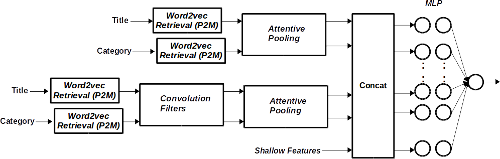
Figure 1. Deep model for Clarity prediction.

The following methods are used to represent a Title or Category as a dense matrix.

Phrase2Mat (P2M)

First, we join the three sub-categories so as to form a single category phrase. Then tokenization is done on a phrase (title or category), removing all out of vocabulary words, and appending the pretrained $word2vec$ ($GoogleNews$) representation [Mikolov et al., 2014] obtained from of the tokens to form the Phrase2Mat matrix.

Hence, we get $\mathbf{T}_{w2v}$ $\in$ $\mathbb{R}^{n\times M}$ for the Title and $\mathbf{C}_{w2v}$ $\in$ $\mathbb{R}^{n\times N}$ for the Category where $M$ and $N$ are lengths of title and category respectively.

Convolutional Neural Network (CNN)

We also use a $CNN$ to get another set of dense representation for a phrase [Kim, 2014]. In particular, a $filter$ $\mathbf{W}$ $\in$ $\mathbb{R}^{n\times h}$ with tanh activation is applied to a window of $h$ words to produce a feature. Thus, for any matrix $\mathbf{X}=[\mathbf{x}_{1},\mathbf{x}_{2},...,\mathbf{x}_{N}]$ where $\mathbf{x}_{i}$ $\in$ $\mathbb{R}^{n}$, applying the filter $\mathbf{W}$ with a stride of 1 gives us $N-h+1$ features. Applying $F$ such filters on $\mathbf{T}_{w2v}$ and $\mathbf{C}_{w2v}$ defined above gives feature maps $\mathbf{T}_{cnn}$ and $\mathbf{C}_{cnn}$ $\in$ $\mathbb{R}^{F\times(N-h+1)}$

To get vectorized representation from matrices, various pooling methods may be used (such as $AveragePooling$ and $MaxPooling$). We use $AttentivePooling$ method which is much more sophisticated.

Attentive Pooling (AttnP)

Attentive pooling [dos Santos et al., 2016] is a way of pooling which allows the pooling operation to be aware of the input pair, in a way that information from the category can directly influence the computation of the title representation $\mathbf{r}^{T}$, and vice versa. Thus, given a $(Title,Category)$ matrix pair $(\mathbf{T},\mathbf{C})$, our aim is to find corresponding vector representation $(\mathbf{r}^{T},\mathbf{r}^{C})$.

Given input matrices $\mathbf{T}$ and $\mathbf{C}$, we try to find a soft alignment between $\mathbf{T}$ ($Title$) and $\mathbf{C}$ ($Category$) after which a weighted average pooling is applied.

A detailed explanation of this approach can be found in [dos Santos et al., 2016].

Thus, from attentive pooling, we obtain $(\mathbf{r}^{T_{w2v}},\mathbf{r}^{C_{w2v}})$ and $(\mathbf{r}^{T_{cnn}},$
$\mathbf{r}^{C_{cnn}})$ from $(\mathbf{T}_{w2v},\mathbf{C}_{w2v})$ and $(\mathbf{T}_{cnn},\mathbf{C}_{cnn})$ respectively.

The final representation $\mathbf{r}^{final}$ $\in$ $\mathbb{R}^{2n+2F+sh}$ is obtained by stacking the representation obtained from the deep network with the engineered features from the Shallow Approach. Here $sh$ is the number of engineered features.

This final representation $\mathbf{r}^{final}$ is given as input to a fully connected Neural Network with $ReLu$ activation in the hidden layers and two neurons with $softmax$ activation as final output. We use the $Adam$ optimizer to train this fully connected network by minimizing the cross-entropy loss. We also used $dropout$ for regularization.

The various hyperparameter setting for this model is given in Table 4 of Appendix A.

4.1.2. Shallow Approach-CLR

For clarity, we use 24 features given as: Given features (1 to 6), Title Counts (7 to 11), and 15, 16, Title Category semantic matching (28 to 30), Title category Matrix(37 to 39), Other features(40), and Deep features (42 to 45) and we use LightGBM package  proposed by [Meng et al., 2016] as a classification algorithm.

4.2. Conciseness

4.2.1. Deep Approach-CON

An overview of the deep model is given in Figure 2

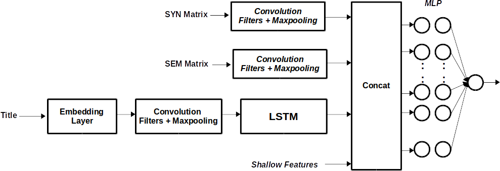
Figure 2. Deep model for Conciseness prediction.

Intra-Title Features (ITF)

To predict Conciseness, we utilised the features contained in the Title only and use features which capture Intra-Title relations. To do this, we extract the semantic and syntactic relationships between tokens in a Title by generating two matrices $\mathbf{SEM}$ and $\mathbf{SYN}$ respectively.

Semantic Relation:

We tokenize the Title and compute the $cosine$ distance between the $word2vec$ representation of all possible pair of tokens. This gives us a symmetric matrix $\mathbf{SEM}$ $\in$ $\mathbb{R}^{N\times N}$ where $N$ is the maximum length of a Title.

Syntactic Relation:

We tokenize the Title and compute the Jaro-Winkler distance [Winkler, 1999] between all possible pair of tokens. This gives us a symmetric matrix $\mathbf{SYN}$ $\in$ $\mathbb{R}^{N\times N}$ where $N$ is the maximum length of a Title.

We remove all out of vocabulary words in generating both the above matrices.

For computing the matrices, the intuition is that, given a Title, we need to know how related/unrelated are the tokens in it. A non-concise title will typically have more noisy tokens or tokens that don’t have much relation with the rest of the title. Hence, we propose that looking at the pairwise relations (semantic/syntactic) between tokens can give an overall picture of the coherence of a title. This relation is precisely represented by the SEM and SYN matrix.

A dense representation is obtained from these relation matrices by using a CNN on them. A convolution with a filter $\mathbf{W}$ $\in$ $\mathbb{R}^{N\times h}$ with tanh activation is applied to both $\mathbf{SEM}$ and $\mathbf{SYN}$ with a stride 1 to give feature maps $\mathbf{F}_{SEM}$ and $\mathbf{F}_{SYN}$ $\in$ $\mathbb{R}^{F\times(N-h+1)}$.

We then apply a max-over-time pooling operation [Collobert and Weston, 2008] over each row of the feature map to obtain final representations $\mathbf{r}^{SEM}$ and $\mathbf{r}^{SYN}$ $\in$ $\mathbb{R}^{F}$ respectively.

CNN-LSTM on Title

We also use a CNN and an LSTM [Zhou et al., 2015] together, directly on the title to get a deep representation of the same. A title of length $N$ is passed through an embedding layer to get a matrix $\mathbf{X}_{title}$ $\in$ $\mathbb{R}^{n\times N}$ where $n$ is the embedding dimension. These embeddings are initialized to word2vec-GoogleNews and fine-tuned during training (We also experimented without tuning the embeddings and Table 1 (b) contains results for both).

A CNN filter $\mathbf{W}$ $\in$ $\mathbb{R}^{n\times h}$ with tanh activation is applied to $\mathbf{X}_{title}$ with stride 1 to obtain a feature map $\mathbf{F}_{title}$ $\in$ $\mathbb{R}^{F\times(N-h+1)}$. To this feature map, a max-over-time-pooling is applied with a pool size of 2 to obtain a matrix $\mathbf{Y}$ $\in$ $\mathbb{R}^{F\times(N-h+1)/2}$ which serves as an input to the LSTM [Hochreiter and Schmidhuber, 1997]. The LSTM has F timesteps. The output of the last timestep of the LSTM is $\mathbf{r}^{CNN-LSTM}$ $\in$ $\mathbb{R}^{hl}$ where $hl$ is the number of hidden units in the LSTM.

The final representation $\mathbf{r}^{final}$ $\in$ $\mathbb{R}^{hl+2F+sh}$ is obtained by stacking $\mathbf{r}^{SEM}$, $\mathbf{r}^{SYN}$, $\mathbf{r}^{CNN-LSTM}$ and the engineered features from the Shallow Approach. Here $sh$ is the number of engineered features. This final representation $\mathbf{r}^{final}$ is given as input to a fully connected Neural Network with $ReLu$ activation in the hidden layers and a single neuron with $sigmoid$ activation as final output. We use the $Adam$ optimizer to train this fully connected network by minimizing the cross-entropy loss. We also used $dropout$ for regularization.

The various hyperparameter setting for this model is given in Table 4 of Appendix A.

4.2.2. Shallow Approach-CON

For conciseness, we use all the features mentioned in section 3 except Title category Matrix features and use LightGBM algorithm as a classification algorithm.

5. Lessons Learnt

One of the key observations is that a simple weighted average of the output of the Shallow and Deep approaches give better results than the two alone suggesting that the results of the two are highly complementary. However, Stacking, which is a common method of learning a good ensemble of models did not give good results. This suggests that although the features from the deep and shallow approaches capture complementary information, we need to look into ways of ensemble them properly.

In particular, we observed that Shallow Learning does better in places where the Title is either too short or when a title comprises of too many numerals and proper nouns which clearly is a problem of out of vocabulary words for Deep Learning.

In contrast, Deep Learning does better than Shallow Learning when the Title is quite long with unnecessary words and hence non-concise. On similar grounds, if a title is long, has fewer proper nouns and is concise/clear, Deep Learning does a better job in classifying them correctly.

We observe that predicting the clarity of a title more sensitive as compared to predicting conciseness because adding/removing even small number features effects highly on clarity score. Hence, in the shallow model as well as deep model, we use less number features for clarity as compared to conciseness.

6. Analysis

We tried different combinations of the approaches described in 4. Due to the fact that some approaches were tried on the validation set while others on the test set, it is difficult to compare them. Hence, the results reported in this section for the Deep and Shallow approaches are on the Holdout set. The final best result is also shown on the provided test set.

P2M + Average Pooling	0.2360
P2M + AttnP	0.2318
CNN + MaxPooling	0.2295
CNN + AttnP	0.2293
P2M + CNN + AttnP	0.2272
P2M + Average Pooling + Shallow Features	0.2340
P2M + AttnP + Shallow Features	0.2304
CNN + MaxPooling + Shallow Features	0.2295
CNN + AttnP + Shallow Features	0.2277
P2M + CNN + AttnP + Shallow Features	0.2265

(a) Clarity

P2M + CNN + AttnP + Shallow Features (w/o tuning)	0.3466
P2M + CNN + AttnP + Shallow Features (tuning)	0.3471
CNN on Title + Shallow Features (w/o tuning)	0.3433
CNN on Title + Shallow Features (tuning)	0.3416
ITF + Shallow Features (w/o tuning)	0.3532
ITF + Shallow Features (tuning)	0.3531
CNN-LSTM on Title + Shallow Features (w/o tuning)	0.3430
CNN-LSTM on Title + Shallow Features (tuning)	0.3420
ITF + CNN-LSTM + Shallow Features (tuning)	0.3379

(b) Conciseness

Table 1. Deep Learning Results on Holdout set in RMSE

Methods:	Clarity		Conciseness
	Holdout set	Test set	Holdout set	Test set
Deep Approach	0.2265	0.2465	0.3379	0.3505
Shallow Approach	0.2271	0.2468	0.3295	0.3477
Ensemble	0.2191	0.2438	0.3187	0.3385

Table 2. Final results on Test and Holdout Set in RMSE.

6.1. Deep Approach

The results for different combination of approaches tried for Clarity and conciseness are presented in Table 1. The representation obtained from these ($\mathbf{r}^{final}$) are fed in to a Deep Neural Network as already explained in 4.

We used a Quadro M3000M GPU machine (4 GB) for training which took around 3 minutes of training time for Clarity and 5.5 minutes of training time for Conciseness.

6.2. Shallow Approach

Table 5 of Appendix A shows the parameters used in LightGBM algorithm for both conciseness and clarity prediction. We also use different algorithms using same set of features. Table 3 compares RMSE over holdout set using different algorithms. It shows that LightGBM outperform rest of the boosting and bagging techniques.

Algorithms	RMSE-CLR	RMSE-CON
Random Forest	0.2356	0.3465
GBM	0.2305	0.3315
XGBoost	0.2283	0.3305
LightGBM	0.2271	0.3295

Table 3. Shallow Learning results on Holdout set in RMSE.

6.3. Ensemble

The final result on holdout and test set is shown in 2. The results shown in this table are for the best performing models for both the Shallow and Deep approaches. In the weighted ensemble for clarity, we use weights 0.55 and 0.45 for predicted probabilities from Deep and Shallow models respectively. For conciseness, we simply take the average (with weights 0.5) of the predicted probabilities.

7. Conclusion

In this report, we have described the various approachs that we used for the ”CIKM AnalytiCup 2017 – Lazada Product Title Quality Challenge”. As the final results prove, a weighted ensemble of Deep and Shallow Models outperform the individual approaches and hence set up a case for future work to learn a better ensemble of these models.

Appendix A Hyperparameter settings

Hyperparameter (Clar/Cons)	Clarity	Conciseness
Word2Vec Embedding Dimension ($n$ / $n$)	300	300
Maximum Title Length ($M$ / $N$)	45	45
Maximum Category Length ($N$ / - )	10	-
Filter Window Width ($h$ / $h$)	3	3
Number of filters ($F$ / $F$)	100	128
Dropout in CNN	0.2	0.2
Dropout in LSTM (- / $hl$)	-	0.2
Dropout in Embedding Layer	-	0.5
Hidden units in LSTM	-	128
Hidden Layers in Neural Net	5	3
Hidden Layer dimension in Neural Net	10	50
Learning Rate	0.0001	0.0001

Table 4. Hyperparameter setting for Deep Learning.

Parameter	Clarity	Conciseness
Learning Rate	0.03	0.03
Colsample Bytree	0.6	0.65
Max Depth	6	-1
Min Child Samples	10	10
n Estimators	390	490
Num Leaves	50	55
Subsample	0.88	0.88
Max Bin	255	255

Table 5. Hyperparameter setting for Shallow Learning.

References

- [1]
- Collobert and Weston [2008] Ronan Collobert and Jason Weston. 2008. A unified architecture for natural language processing: Deep neural networks with multitask learning. In Proceedings of the 25th international conference on Machine learning. ACM, 160–167.
- Collobert et al. [2011] Ronan Collobert, Jason Weston, Léon Bottou, Michael Karlen, Koray Kavukcuoglu, and Pavel Kuksa. 2011. Natural language processing (almost) from scratch. Journal of Machine Learning Research 12, Aug (2011), 2493–2537.
- dos Santos et al. [2016] Cıcero Nogueira dos Santos, Ming Tan, Bing Xiang, and Bowen Zhou. 2016. Attentive pooling networks. CoRR, abs/1602.03609 (2016).
- Hochreiter and Schmidhuber [1997] Sepp Hochreiter and Jürgen Schmidhuber. 1997. Long short-term memory. Neural computation 9, 8 (1997), 1735–1780.
- Kim [2014] Yoon Kim. 2014. Convolutional neural networks for sentence classification. arXiv preprint arXiv:1408.5882 (2014).
- Meng et al. [2016] Qi Meng, Guolin Ke, Taifeng Wang, Wei Chen, Qiwei Ye, Zhi-Ming Ma, and Tieyan Liu. 2016. A communication-efficient parallel algorithm for decision tree. In Advances in Neural Information Processing Systems. 1279–1287.
- Mikolov et al. [2014] Tomas Mikolov, Kai Chen, Greg Corrado, Jeffrey Dean, L Sutskever, and G Zweig. 2014. word2vec. (2014).
- Pennington et al. [2014] Jeffrey Pennington, Richard Socher, and Christopher D. Manning. 2014. GloVe: Global Vectors for Word Representation. In Empirical Methods in Natural Language Processing (EMNLP). 1532–1543. http://www.aclweb.org/anthology/D14-1162
- Winkler [1999] William E Winkler. 1999. The state of record linkage and current research problems. In Statistical Research Division, US Census Bureau.
- Zhou et al. [2015] Chunting Zhou, Chonglin Sun, Zhiyuan Liu, and Francis Lau. 2015. A C-LSTM neural network for text classification. arXiv preprint arXiv:1511.08630 (2015).