On the existence of non-trivial steady-state size-distributions for a class of flocculation equations

Abstract

Flocculation is the process whereby particles (i.e., flocs) in suspension reversibly combine and separate. The process is widespread in soft matter and aerosol physics as well as environmental science and engineering. We consider a general size-structured flocculation model, which describes the evolution of floc size distribution in an aqueous environment. Our work provides a unified treatment for many size-structured models in the environmental, industrial, medical, and marine engineering literature. In particular, the mathematical model considered in this work accounts for basic biological phenomena in a population of microorganisms including growth, death, sedimentation, predation, surface erosion, renewal, fragmentation and aggregation. The central objective of this work is to prove existence of positive steady states of this generalized flocculation model. Using results from fixed point theory we derive conditions for the existence of continuous, non-trivial stationary solutions. We further develop a numerical scheme based on spectral collocation method to approximate these positive stationary solutions. We explore the stationary solutions of the model for various biologically relevant parameters and give valuable insights for the efficient removal of suspended particles.

1 Introduction

Flocculation is the process whereby particles (i.e., flocs) in suspension reversibly combine and separate. The process is widespread in soft matter and aerosol physics as well as environmental science and engineering. For instance, in fields such as water treatment, biofuel production and beer fermentation, flocculation process is often used to enhance suspended solids removal. One of the most important design and control parameters for the efficient removal of suspended particles is the size distribution of the flocs in stirring tanks. A popular mathematical model describing the time-evolution of the particle size distribution in a stirring tank is a 1D nonlinear partial integro-differential equation based on the population-balance equations proposed by van Smoluchowski, [45]. The model have been successful in matching many flocculation experiments [25, 14, 41].

Previous analytical work on these models focused on classes of flocculation equations that did not allow for the vital dynamics (i.e., birth and death) of individual particles. These phenomena are obviously critical features in the modeling of microbial flocculation. Accordingly, in this work we consider a general size-structured flocculation model which accounts for growth, aggregation, fragmentation, surface erosion and sedimentation. The equations for the microbial flocculation model track the time-evolution of the particle size number density $u(t,\,x)$ and can be written as

$$u_{t} = \mathcal{F}(u)$$ (1)

where

$$\mathcal{F}(u):=\mathcal{G}(u)+\mathcal{A}(u)+\mathcal{B}(u),$$

$\mathcal{G}$ denotes growth

$$\mathcal{G}(u):=-\partial_{x}(gu)-\mu(x)u(t,\,x)\,,$$ (2)

$\mathcal{A}$ denotes aggregation

$$\mathcal{A}(u) :=\frac{1}{2}\int_{0}^{x}k_{a}(x-y,\,y)u(t,\,x-y)u(t,\,y)\,dy$$

$$\quad-u(t,\,x)\int_{0}^{\overline{x}-x}k_{a}(x,\,y)u(t,\,y)\,dy\,,$$ (3)

and $\mathcal{B}$ denotes breakage

$$\mathcal{B}(u):=\int_{x}^{\overline{x}}\Gamma(x;\,y)k_{f}(y)u(t,\,y)\,dy-\frac{1}{2}k_{f}(x)u(t,\,x)\,.$$ (4)

The boundary condition is traditionally defined at the smallest size $0$ and the initial condition is defined at $t=0$

$$g(0)u(t,\,0)=\int_{0}^{\overline{x}}q(x)u(t,\,x)dx,\quad u(0,\,x)=u_{0}(x)\,,$$

where the renewal rate $q(x)$ represents the number of new flocs entering the population. We note that this boundary condition could also be used to model the surface erosion of flocs, where single cells are eroded off the floc and enter single cell population. A floc size is usually expressed as volume. Moreover, since the equations model flocculation of particles in a confined space, the flocs are assumed to have a maximum size $\overline{x}<\infty$. The function $g(x)$ represents the average growth rate of the flocs of size $x$ due to proliferation, and the coefficient $\mu(x)$ represents a size-dependent removal rate due to gravitational sedimentation and death.

The aggregation of flocs into larger ones is modeled in (3), by the Smoluchowski coagulation equation. The function $k_{a}(x,\,y)$ is the aggregation kernel, which describes the rate with which the flocs of size $x$ and $y$ agglomerate to form a floc of size $x+y$. This equation has been widely used, e.g., to model the formation of clouds and smog in meteorology [35], the kinetics of polymerization in biochemistry [47], the clustering of planets, stars and galaxies in astrophysics [26], and even schooling of fish in marine sciences [33]. The equation has also been the focus of considerable mathematical analysis. For the aggregation kernels satisfying the inequality $k_{a}(x,\,y)\leq 1+x+y$, existence of mass conserving global in time solutions were proven [13, 20, 28] (for some suitable initial data). Conversely, for aggregation kernels satisfying $(xy)^{\gamma/2}\leq k_{a}(x,\,y)$ with $1<\gamma\leq 2$, it has been shown that the total mass of the system blows up in a finite time (referred as a gelation time) [15]. For a review of further mathematical results, we refer readers to review articles by Aldous [3], Menon and Pego [29], and Wattis [46] and the book by Dubovskii [12]. Lastly, although the Smoluchowski equation has received substantial theoretical work, the derivation of analytical solutions for many realistic aggregation kernels has proven elusive. Towards this end, many discretization schemes for numerical simulations of the Smoluchowski equations have been proposed, and we refer interested readers to the review by Bortz [6, §6].

The breakage of flocs due to fragmentation is modeled by the terms in (4), where the fragmentation kernel $k_{f}(x)$ calculates the rate with which a floc of size $x$ fragments. The breakage process assumes the fragmentation of a floc of size $x$ into sizes $\{x-y,\,y\}$ and $\{y,\,x-y\}$ as two separate events. Therefore, the factor of $1/2$ is included in the second sum to avoid double-counting. The integrable function $\Gamma(x;y)$ represents the post-fragmentation probability density of daughter flocs for the fragmentation of the parent flocs of size $y$. The post-fragmentation probability density function $\Gamma$ is one of the least understood terms in the flocculation model. Many different forms are used in the literature, among which normal and log-normal densities are the most common [43]. Recent modeling and computational work suggests that normal and log-normal forms for $\Gamma$ are not correct and that a form closer to an $\arcsin(x;y)$ density would be more accurate [31, 8]. However, in this work we do not restrict ourselves to any particular form of $\Gamma$, and instead simply assume that the function $\Gamma$ satisfies the mass conservation requirement. In other words, all the fractions of daughter flocs formed upon the fragmentation of a parent floc sum to unity,

$$\int_{0}^{y}\Gamma(x;\,y)\,dx=1\text{ for all }y\in(0,\,\overline{x}].$$ (5)

The microbial flocculation equation, presented in (1), is a generalization of many mathematical models appearing in the size-structured population modeling literature and has been widely used, e.g., to model the formation of clouds and smog in meteorology [35], the kinetics of polymerization in biochemistry [47], the clustering of planets, stars and galaxies in astrophysics [26], and even schooling of fish in marine sciences [33]. For example, when the fragmentation kernel is omitted, $k_{f}\equiv 0$, the flocculation model reduces to algal aggregation model used to describe the evolution of a phytoplankton community [2]. When the removal and renewal rates are set to zero, the flocculation model simplifies to a model used to describe the proliferation of Klebsiella pneumonia in a bloodstream [7]. Furthermore, the flocculation model, with only growth and fragmentation terms, was used to investigate the elongation of prion polymers in infected cells [9, 11, 10].

Investigating asymptotic behavior of the equation (1) has been a challenging task because of the nonlinearity introduced by the aggregation terms. Nevertheless, under suitable conditions on the kernels, the existence of a positive steady state has been established for the pure aggregation and fragmentation case [24]. For the case $\overline{x}=\infty$, [4] establishes that for certain range of parameters, the solutions of the flocculation model do blow up in finite time. To the best of our knowledge, for the case $\overline{x}<\infty$ the long-term behavior of this model has not been considered. Hence, our main goal in this paper is to rigorously investigate the long-term behavior of the broad class of flocculation models described in (1).

When the long-term behavior of biological populations is considered, many populations converge to a stable time-independent state. Thus, identifying conditions under which a population converges to a stationary state is one of the most important applications of mathematical population modeling. Hence, our main goal in this work is to prove existence of positive steady states of the microbial flocculation model (1). It is trivially true that a zero stationary solution of the microbial flocculation model exists, but we are also interested in non-trivial stationary solutions of the microbial flocculation model. Consequently, in Section 2 we first show that under some suitable conditions on the model parameters the equation (1) has at least one non-trivial (non-zero and non-negative) stationary solution. In Section 3, we present a numerical scheme to approximate these stationary solutions. The numerical scheme is based on spectral collocation method, and thus yields very accurate results even for small approximation dimensions. Furthermore, we explore the stationary solutions of the model for various biologically relevant parameters in Section 4 and give valuable insights for the efficient removal of suspended particles.

2 Existence of a positive stationary solution

The flocculation model under our consideration (1), accounts for physical mechanisms such as growth, removal, fragmentation, aggregation and renewal of microbial flocs. Thus, under some conditions, which balance these mechanisms, one could reasonably expect that the model possesses a non-trivial stationary solution. Hence, our main goal in this section is to derive sufficient conditions for the model terms such that the equation (1) engenders a positive stationary solution.

The flocculation model in this form (1) was first considered by Banasiak and Lamb in [5], where they employed the flocculation model to describe the dynamical behavior of phytoplankton cells. The authors showed that under some conditions the flocculation model is well-posed, i.e., there exist a unique, global in time, positive solution for every absolutely integrable initial distribution. For the remainder of this work, we make the following assumptions on the model rates for which well-posedness of the solutions of the microbial flocculation equations has been established by Banasiak and Lamb, [5]:

$$(\mathbf{A}1)\qquad g\in C^{1}(I)\qquad g(x)>0\>\text{ for }x\in I=[0,\,\overline{x}]$$

$$(\mathbf{A}2)\qquad k_{a}\in L^{\infty}(I\times I),\quad k_{a}(x,\,y)=k_{a}(y,\,x)$$

$$\text{ and }k_{a}(x,\,y)=0\,\,\,\text{ if }x+y\geq\overline{x}\,,$$

$$(\mathbf{A}3)\qquad \mu\in C(I)\qquad\text{and }\mu\geq 0\text{ a.e. on }I\,,$$

$$(\mathbf{A}4)\qquad q\in L^{\infty}(I)\qquad\text{and }q\geq 0\text{ a.e. on }I\,,$$

$$(\mathbf{A}5)\qquad k_{f}\in C(I)\qquad k_{f}(0)=0\text{ and }k_{f}\geq 0\text{ a.e. on }I\,,$$

$$(\mathbf{A}6)\qquad \Gamma(\cdot,\,y)\in L^{\infty}(I),\quad\Gamma(x;\,y)\geq 0\text{ for }x\in(0,\,y];$$

$$\text{and }\Gamma(x;\,y)=0\text{ for }x\in(y,\,\overline{x})\,.$$

Assumption ($\mathbf{A}1$) states that the floc of any size has strictly positive growth rate. This in turn implies that flocs can grow beyond the maximal size $\overline{x}$, i.e., the model ignores what happens beyond the maximal size $\overline{x}$ (as many authors in the literature have done [1, 16, 2]). We also note that although the Assumption $(\mathbf{A}1)$ is widely used in the literature it does generate biologically unrealistic condition $g(0)>0$, i.e., the flocs of size zero also have positive growth rate. However, this assumption is crucial for our work, and thus we postpone the analysis of the case $g(0)=0$ for our future research. Assumption $(\mathbf{A}2)$ states that for the aggregates of size $x$ and $y$ the aggregation rate is zero if the combined size of the aggregates is larger than the maximal size. Lastly, Assumption $(\mathbf{A}3)$ on $\mu(x)$ enforces continuous dependence of the removal on the size of a floc and ensures that every floc is removed with a non-negative rate.

Recall that at a steady state we should have

$$u_{t}=0=\mathcal{F}[u]\,.$$ (6)

By Assumption $(\mathbf{A}1)$, we know that $1/g\in C(I)$ and thus we can define $u=f/g$ for some $f\in C(I)$. The substitution of this $f$ into (6), integration between $0$ and an arbitrary $x$, and rearrangment of the terms yields

$$f(x) =f(0)-\int_{0}^{x}\frac{k_{f}(y)/2+\mu(y)}{g(y)}f(y)\,dy+\int_{0}^{x}\int_{z}^{\overline{x}}\frac{\Gamma(z;\,y)k_{f}(y)}{g(y)}f(y)\,dy\,dz$$

$$\quad+\frac{1}{2}\int_{0}^{x}\int_{0}^{z}\frac{k_{a}(z-y,\,y)}{g(z-y)g(y)}f(z-y)f(y)\,dy\,dz-\int_{0}^{x}\frac{f(z)}{g(z)}\int_{0}^{\overline{x}}\frac{k_{a}(z,\,y)}{g(y)}f(y)\,dy\,dz\,.$$ (7)

At this point we set

$$f(0)=1=g(0)p(0)=\int_{0}^{\overline{x}}q(y)u(y)\,dy\,.$$ (8)

Note that if there is a function $f$ satisfying the equations (7) and (8), then $u_{*}$ is a steady state for the modified choice of $q(x)$

$$q(x):=\frac{q(x)}{\int_{0}^{\overline{x}}\frac{q(y)f(y)}{g(y)}\,dy}\,.$$ (9)

We now define the operator $\Phi$ as

$$\Phi[f](x) :=1-\int_{0}^{x}\frac{k_{f}(y)/2+\mu(y)}{g(y)}f(y)\,dy+\int_{0}^{x}\int_{z}^{\overline{x}}\frac{\Gamma(z;\,y)k_{f}(y)}{g(y)}f(y)\,dy\,dz$$

$$\quad+\frac{1}{2}\int_{0}^{x}\int_{0}^{z}\frac{k_{a}(z-y,\,y)}{g(z-y)g(y)}f(z-y)f(y)\,dy\,dz-\int_{0}^{x}\frac{f(z)}{g(z)}\int_{0}^{\overline{x}}\frac{k_{a}(z,\,y)}{g(y)}f(y)\,dy\,dz\,.$$ (10)

and will use a fixed point theorem to prove the existence of a fixed point $f$ of $\Phi$ . This in turn will allow us to claim that equation (6) has at least one non-trivial positive solution.

The use of fixed point theorems for showing existence of non-trivial stationary solutions is not new in size-structured population modeling. For example, fixed point theorems, based on Leray-Schauder degree theory, have been used to find stationary solutions of linear Sinko-Streifer type equations [36, 17]. Moreover, the Schauder fixed point theorem has been used to establish the existence of steady state solutions of nonlinear coagulation-fragmentation equations [23]. For our purposes we will use the Contraction Mapping Theorem.

We carry out the analysis of this work on the space of continuous functions $\mathcal{X}=C(I)$ with usual uniform (supremum) norm $\left\|\cdot\right\|_{u}$. We also denote the usual essential supremum of a function by $\left\|\cdot\right\|_{\infty}$. Since the positive cone in $C(I)$, denoted by $\left(C(I)\right)_{+}$, is closed and convex, we choose $K$ to be $\left(C(I)\right)_{+}$. Then $K_{r}=\overline{K\cap B_{r}(0)}$, where $B_{r}(0)\subset\mathcal{X}$ is an open ball of radius $r$ and centered at zero, and $r$ has yet to be chosen. Note that since $K_{r}$ is also Banach space since it is closed subspace of $\mathcal{X}$. Next, we show that one can choose model rates such that the operator $\Phi$ defined in (10) maps $K_{r}$ to $K_{r}$ and is also contraction. This in turn implies existence of a positive stationary solution of the operator $\mathcal{F}$. We are now in a position to state the main result of this section in the following theorem.

Theorem 2.1.

Assume that the condition

$$0\leq\frac{1}{2}k_{f}(x)-\mu(x),$$

holds true for all $x\in I$. For sufficiently small choice of $\left\|\frac{1}{g}\right\|_{1}$ the operator $\Phi$ defined in (10) has a unique non-zero fixed point, $f_{*}\in K$ satisfying

$$1\leq\left\|f_{*}\right\|_{u}\leq r$$ (11)

for some $r\geq 1$. Moreover, for the modified choice of the renewal rate in (9), the non-zero and non-negative function

$$u_{*}=\frac{f_{*}}{g}\in C(I)$$ (12)

is a unique stationary solution of the flocculation model defined in (1) on $K$.

Proof.

For $f\in K_{r}$ we have

$$\Phi[f] \geq 1-\int_{0}^{x}\frac{k_{f}(y)/2+\mu(y)}{g(y)}f(y)\,dy$$

$$\quad+\int_{0}^{x}\int_{z}^{x}\frac{\Gamma(z;\,y)k_{f}(y)}{g(y)}f(y)\,dy\,dz-\int_{0}^{x}\frac{f(z)}{g(z)}\int_{0}^{\overline{x}}\frac{k_{a}(z,\,y)}{g(y)}f(y)\,dy\,dz$$

$$\geq 1-\int_{0}^{x}\frac{f(z)}{g(z)}(k_{f}(z)/2+\mu(z))\,dz+\int_{0}^{x}\frac{k_{f}(y)f(y)}{g(y)}\underbrace{\int_{0}^{y}\Gamma(z;\,y)\,dz}_{=1}\,dy-\left\|f\right\|_{u}^{2}\left\|k_{a}\right\|_{\infty}\left\|\frac{1}{g}\right\|_{1}^{2}$$

$$\geq\int_{0}^{x}\frac{f(z)}{g(z)}\left(\frac{1}{2}k_{f}(z)-\mu(z)\right)\,dz\,+1-r^{2}\cdot\left\|k_{a}\right\|_{\infty}\left\|\frac{1}{g}\right\|_{1}^{2},$$

where $\left\|\cdot\right\|_{1}$ represents the usual $L^{1}$ norm on $I$. The first condition of the theorem $(\mathbf{C}1)$ guarantees that

$$\frac{1}{2}k_{f}(z)-\mu(z)>0\text{ for all }z\in I\,,$$

so we can choose

$$r=\left\|\frac{1}{g}\right\|_{1}^{-1}\left\|k_{a}\right\|_{\infty}^{-1/2}$$ (13)

in $K_{r}$ such that $\Phi[f]\geq 0$, i.e., $\Phi\,:\,K_{r}\to K$. On the other hand, using the assumptions $(\mathbf{A}1)$-$(\mathbf{A}6)$, it is straightforward to show that $\Phi(K_{r})\subset C(I)$.

Next we prove that the operator $\Phi$ maps $K_{r}$ to $K_{r}$. Consequently, for $f\in K_{r}$ it follows that

$$0\leq\Phi[f](x) \leq 1-\int_{0}^{x}\frac{k_{f}(y)/2+\mu(y)}{g(y)}f(y)\,dy+\int_{0}^{\overline{x}}\int_{z}^{\overline{x}}\frac{\Gamma(z;\,y)k_{f}(y)}{g(y)}f(y)\,dy\,dz$$

$$\quad-\int_{x}^{\overline{x}}\int_{z}^{\overline{x}}\frac{\Gamma(z;\,y)k_{f}(y)}{g(y)}f(y)\,dy\,dz+\frac{1}{2}\int_{0}^{x}\int_{0}^{z}\frac{k_{a}(z-y,\,y)}{g(z-y)g(y)}f(z-y)f(y)\,dy\,dz$$

$$\leq 1+\int_{x}^{\overline{x}}\frac{1}{g(y)}k_{f}(y)f(y)\,dy+\int_{0}^{x}\frac{1}{g(y)}\left(\frac{1}{2}k_{f}(y)-\mu(y)\right)f(y)\,dy$$

$$\quad+\frac{1}{2}\left\|f\right\|_{u}^{2}\cdot\left\|k_{a}\right\|_{\infty}\cdot\left\|\frac{1}{g}\right\|_{1}^{2}$$

$$\leq 1+\left\|f\right\|_{u}\left\|\frac{1}{g}\right\|_{1}\left[\left\|k_{f}\right\|_{u}+\left\|\frac{1}{2}k_{f}-\mu\right\|_{u}+r\left\|k_{a}\right\|_{\infty}\left\|\frac{1}{g}\right\|_{1}\right]$$

$$\leq 1+r\left\|\frac{1}{g}\right\|_{1}\left[\left\|k_{f}\right\|_{u}+\left\|\frac{1}{2}k_{f}-\mu\right\|_{u}+\left\|k_{a}\right\|_{\infty}^{1/2}\right]\,.$$

At this point choosing $\left\|\frac{1}{g}\right\|_{1}$ sufficiently small yields $r>1$ in (13), and thus we can guarantee that

$$\left\|\Phi[f]\right\|\leq r$$

for all $f\in K_{r}$. Hence the operator $\Phi$ maps $K_{r}$ to $K_{r}$.

Next we will prove that the operator $\Phi$ is in fact a contraction mapping, i.e., for all $f,\,h\in K_{r}$

$$\left\|\Phi[f]-\Phi[h]\right\|_{u}\leq c\left\|f-h\right\|_{u}$$

for some $c\in[0,1)$.

$$\left|\Phi[f](x)-\Phi[h](x)\right| \leq\int_{0}^{x}\frac{k_{f}(y)/2-\mu(y)}{g(y)}\left|f(y)-h(y)\right|\,dy+\int_{x}^{\overline{x}}\frac{k_{f}(y)}{g(y)}\left|f(y)-h(y)\right|\,dy$$

$$+\frac{1}{2}\int_{0}^{x}\int_{0}^{z}\frac{k_{a}(z-y,\,y)}{g(z-y)g(y)}f(z-y)\left|f(y)-h(y)\right|\,dy\,dz$$

$$+\frac{1}{2}\int_{0}^{x}\int_{0}^{z}\frac{k_{a}(z-y,\,y)}{g(z-y)g(y)}h(y)\left|f(z-y)-h(z-y)\right|\,dy\,dz$$

$$+\int_{0}^{x}\frac{f(z)}{g(z)}\int_{0}^{\overline{x}}\frac{k_{a}(z,\,y)}{g(y)}\left|f(y)-h(y)\right|\,dy\,dz$$

$$+\int_{0}^{x}\frac{\left|f(z)-h(z)\right|}{g(z)}\int_{0}^{\overline{x}}\frac{k_{a}(z,\,y)}{g(y)}h(y)\,dy\,dz\,.$$

Taking the supremum of both sides at this point yields

$$\left\|\Phi[f]-\Phi[h]\right\|_{u}\leq\left\|f-h\right\|_{u}\left\|\frac{1}{g}\right\|_{1}\left[\left\|k_{f}\right\|_{u}+\left\|\frac{1}{2}k_{f}-\mu\right\|_{u}+\frac{3}{2}\left\|k_{a}\right\|_{\infty}^{1/2}\right]\,.$$

Once again by choosing $\left\|\frac{1}{g}\right\|_{1}$ sufficiently small, we can guarantee that the constant

$$c=\left\|\frac{1}{g}\right\|_{1}\left[\left\|k_{f}\right\|_{u}+\left\|\frac{1}{2}k_{f}-\mu\right\|_{u}+\frac{3}{2}\left\|k_{a}\right\|_{\infty}^{1/2}\right]$$

is less than $1$. This in turn implies that the operator $\Phi$ defined in (10) is also a contraction mapping. Hence, the Contraction Mapping Theorem guarantees the existence of a unique positive fixed point of $\Phi$ satisfying the bounds (11). Therefore, the function $u_{*}=f_{*}/g$ is a stationary solution of the flocculation equations (1). Moreover, from the assumption ($\mathbf{A}1$) and the continuity of the fixed point $f_{*}$ it follows that $u_{*}$ is non-zero, non-negative and continuous on $I$. ∎

3 Numerical approximation of non-trivial stationary solutions

Recall that at steady state the microbial flocculation equations reduce to first order integro-differential equation

$$\partial_{x}(gu_{*}) =\frac{1}{2}\int_{0}^{x}k_{a}(x-y,\,y)u_{*}(x-y)u_{*}(y)\,dy-u_{*}(x)\int_{0}^{\overline{x}-x}k_{a}(x,\,y)u_{*}(y)\,dy$$

$$\quad+\int_{x}^{\overline{x}}\Gamma(x;\,y)k_{f}(y)u_{*}(y)\,dy-\frac{1}{2}k_{f}(x)u_{*}(x)-\mu(x)u_{*}(x)$$ (14)

with a boundary condition

$$g(0)u_{*}(0)=\int_{0}^{\overline{x}}q(x)u_{*}(x)dx\,.$$

This in turn can be expressed in the form of a boundary value problem.

$$\frac{du_{*}}{dx}=F(x,\,u_{*}),\qquad u_{*}(0)=\int_{0}^{\overline{x}}q(x)u_{*}(x)dx/g(0)\,.$$ (15)

If we set

$$\int_{0}^{\overline{x}}q(x)u_{*}(x)dx=1$$

and adjust the renewal rate to the obtained steady state as in Section 2, we get an initial value problem

$$\frac{du_{*}}{dx}=F(x,\,u_{*}),\qquad u_{*}(0)=1/g(0)\,.$$ (16)

Using Picard’s Existence Theorem for IVPs, one can show that the IVP (16) has a unique solution for a suitably chosen interval around the initial condition. Therefore, the above IVP is well-posed. Note that we still need results of Section 2 for the existence of a positive stationary solution since Picard’s Existence Theorem does not guarantee positivity of solutions of (16).

The solutions of the IVP (16) can be approximated using various numerical schemes such as finite difference, finite element, and spectral methods [32, 27, 30]. Towards this end, in this section, we develop a numerical scheme to approximate the solutions of the IVP (16). The numerical scheme is based on spectral collocation method and thus yields very accurate results even for small approximation dimensions.

Spectral collocation method, also known as pseudospectral methods, is a subclass of Galerkin spectral methods [19, 44]. Spectral methods, in general, have higher accuracy compared to Finite difference and Finite Element methods and thus have widespread use for the numerical simulation of partial differential equations. The main idea behind the method is to express numerical solutions as a finite expansion of some set of basis functions on a number of points on the domain (i.e., collocation points). Convergence of the approximations depend only on the smoothness of the solutions and thus the method can attain high precision even with a few grid points.

We approximate the stationary solution $u_{*}(x)$ as linear combination of $N$th degree polynomials $\left\{\phi_{j}(x)\right\}_{j=0}^{N}$, i.e.,

$$\left[I_{N}u_{*}\right](x)=\sum_{j=0}^{N}u_{*}(x_{j})\phi_{j}(x)\,,$$

for some collocation points $\left\{x_{j}\right\}_{j=0}^{N}\subset I$. Furthermore, we require that this approximation is exact at collocation points, i.e.,

$$\phi_{j}(x_{k})=\begin{cases}1&\text{if }j=k\\ 0\,&\text{otherwise}\end{cases}\,.$$

The polynomials $\left\{\phi_{j}(x)\right\}_{j=0}^{N}$ satisfying the above requirements are called cardinal functions. Straightforward way to compute such polynomials is using Lagrangian interpolation, i.e.,

$$\phi_{j}(x)=\frac{\pi(x)}{\pi^{\prime}(x_{j})(x-x_{j})}\,,$$ (17)

where $\pi(x)=\Pi_{j=0}^{N}(x-x_{j})$. Consequently, derivative can be computed as

$$\frac{d}{dx}\left[I_{N}u_{*}\right](x)=\sum_{j=0}^{N}u_{*}(x_{j})\phi_{j}^{\prime}(x)\,.$$

This in turn implies that derivative at $x_{i}$ can be computed as linear combination of $\left\{u_{*}(x_{j})\right\}_{j=0}^{N}$. Plugging in collocation points into above equation yields the differentiation matrix $[D]_{i,\,j}=\phi_{j}^{\prime}(x_{i})$. Entries of $D$ can be computed explicitly as

$$D_{ij}=\frac{\pi^{\prime}(x_{i})}{\pi^{\prime}(x_{j})(x_{i}-x_{j})}$$

for off-diagonal entries $i\neq j$ and

$$D_{jj}=\sum_{\begin{array}[]{c}k=0,\,k\neq j\end{array}}^{N}\frac{1}{x_{j}-x_{k}}\,$$

for diagonal entries. Let $\vec{u}$ denote the vector

$$\begin{bmatrix}u_{*}(x_{0})&\cdots&u_{*}(x_{N})\end{bmatrix}^{T}\,,$$

then derivatives at collocation points are given by

$$\begin{bmatrix}u_{*}^{\prime}(x)&\cdots&u_{*}^{\prime}(x_{N})\end{bmatrix}^{T}=D\vec{u}\,.$$

When a smooth function is interpolated by polynomials in $N$ equally space points, the approximations sometimes fail to converge as $N\to\infty$, which is also known as Runge phenomenon. Moreover, when using uniform gird points, the elements of the differentiation matrix not only fail to converge but they get worse and diverge as $N\to\infty$. For the spectral collocation methods, it is a general consensus to cluster the grid points roughly quadratically toward the endpoints of the interval [19]. Therefore, for collocation points we use unevenly space grid points. We employ non-uniform shifted Chebyshev-Gauss-Lobatto grid points,

$$x_{j}=\left(1-\cos\left(\frac{j\pi}{N}\right)\right)\frac{\overline{x}}{2}\qquad\forall i=0,1,\dots,N\,.$$ (18)

Points $\left\{\cos\left(\frac{j\pi}{N}\right)\right\}_{j=0}^{N}$ are in fact extrema of $N$th Chebyshev polynomial on the interval $-1\leq x\leq 1$.

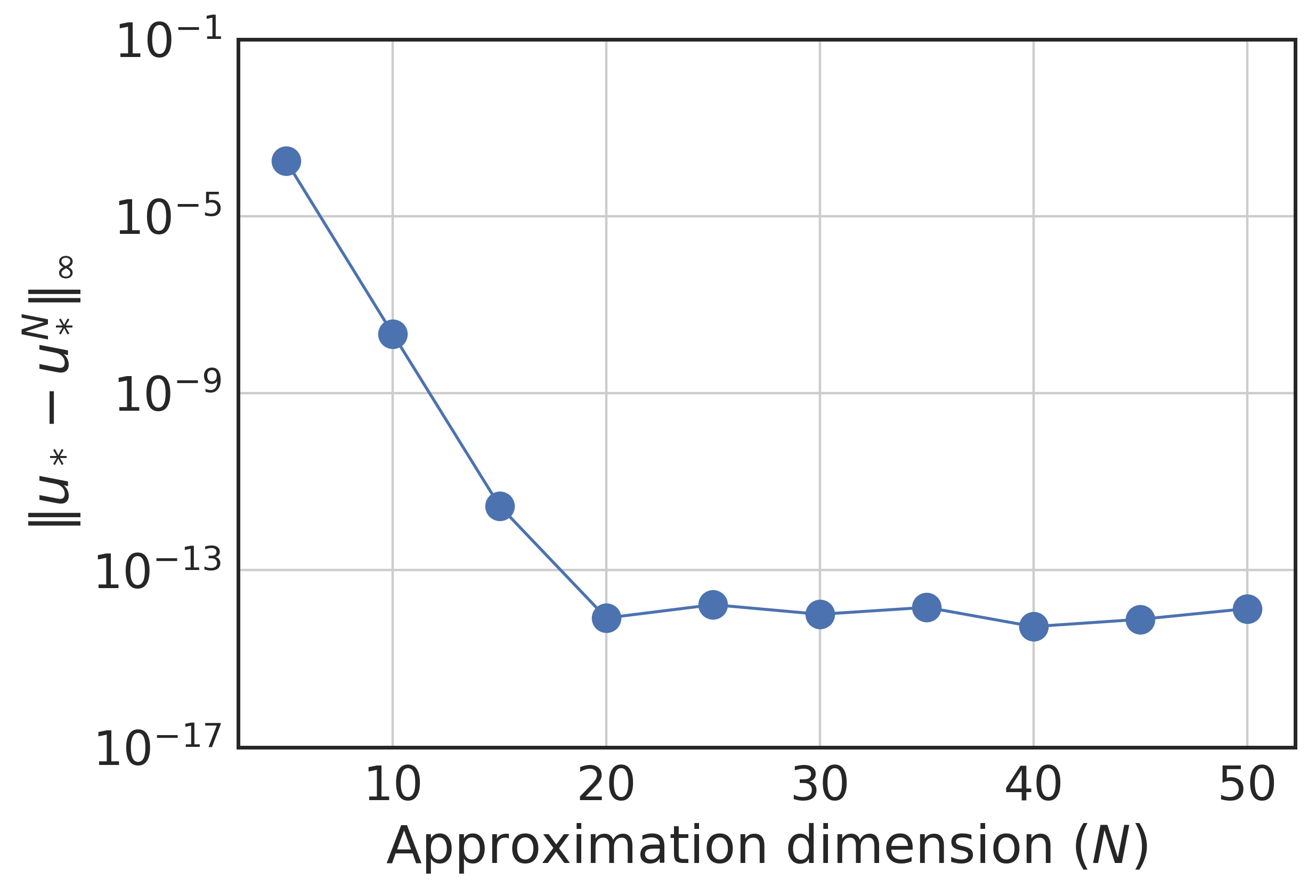
(a)

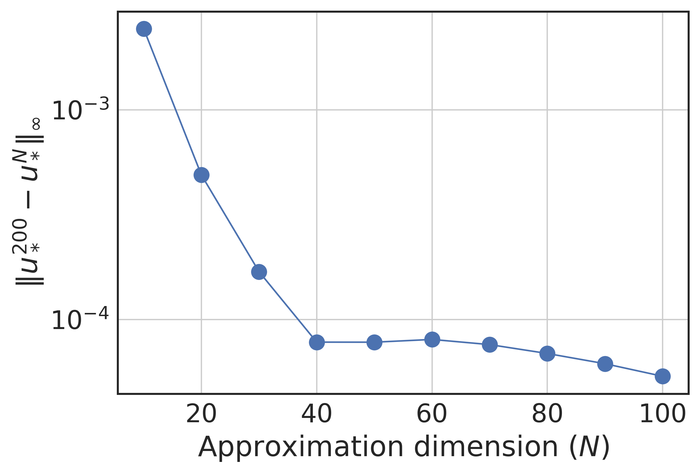
(b)

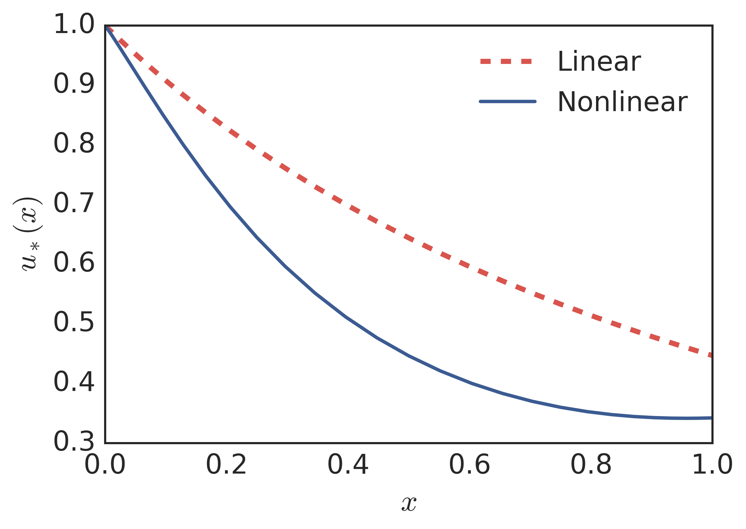
(c)

Figure 1: a) Error in approximation of the steady states of linear Sinko-Streifer. Compared to existing analytical solution. b) Error in approximation of the steady states of nonlinear flocculation equations compared to approximate solution at $N=200$. c) Example steady state solutions for linear Sinko-Streifer equations and nonlinear microbial flocculation equations

For the numerical approximations of the steady state of the microbial flocculation model (1)For integral approximations we used Gaussian quadrature,

$$\int_{0}^{\overline{x}}f(s)\,ds\approx\sum_{i=0}^{N}w_{i}f(x_{i})\,.$$

We require Gaussian quadrature to be exact for chosen cardinal functions $\left\{\phi_{i}(x)\right\}_{i=0}^{N}$, which yields weights

$$w_{i}=\int_{0}^{\overline{x}}\phi_{i}(s)\,ds\,.$$

Moreover, in the evaluation of the integrals in (3) one has to evaluate $\left[I_{N}u_{*}\right](x)$ at non-collocation points, i.e.,

$$\left[I_{N}u_{*}\right](x_{k}-x_{i})=\sum_{j=0}^{N}u_{*}(x_{j})\phi_{j}(x_{k}-x_{i})\,.$$ (19)

Once $\phi_{j}(x_{k}-x_{i})$ are calculated explicitly using (17), the approximations at non-collocation points (19) can be evaluated as linear combination of entries of $\vec{p}$. For efficient implementation the elements $\phi_{j}(x_{k}-x_{i})$ can be initialized as entries of three dimensional array, i.e.,

$$[\Phi]_{k,i,j}=\begin{cases}\phi_{j}(x_{k}-x_{i})&\text{ if }k\geq i\\ 0&\text{otherwise}\end{cases}\,.$$

Consequently, approximation for (19) can be obtained as

$$\left[I_{N}u_{*}\right](x_{k}-x_{i})=\sum_{j=0}^{N}[\Phi]_{k,i,j}\vec{u}_{j}\,,$$

which is simply dot product of three dimensional array $\Phi$ with the vector $\vec{u}$.

To verify convergence of the proposed approximation scheme, we apply first applied our numerical scheme to a special case of flocculation equations for which an exact form of the stationary solution is available. In particular, in the absence of aggregation and fragmentation the flocculation equations simplify to linear Sinko-Streifer model [38]. The model describes the dynamics of single species populations and takes into account the physiological characteristics of animals of different sizes (and/or ages).

Setting the right side of the equation (2) to zero and integrating over the size on $(0,\,x)$ yields the exact stationary solution

$$u_{*}(x)=\frac{1}{g(x)}\exp\left(-\int_{0}^{x}\frac{\mu(s)}{g(s)}\,ds\right)\,.$$ (20)

In Figure 1a, we compared numerical approximations of the stationary solution to exact solution given in (20). The absolute error decreases exponentially fast for increasing approximation dimension $N$. Numerical approximation attains machine precision for $N\geq 20$. As for the full nonlinear flocculation equations, to the best of our knowledge, no analytical starionary solution is available. Therefore, in Figure 1b, we have plotted relative error of approximations compared to a approximation at $N=200$. Relative error decreases fast and achieves four digit precision for $N\geq 40$. Moreover, example steady state solutions for both linear and nonlinear cases are illustrated in Figure 1c.

4 Numerical Exploration of Steady States

Having the approximation scheme in hand, in this section, we explore the stationary solutions of the model for various biologically relevant parameters and give valuable insights for the efficient removal of suspended particles. For the purpose of illustration, the aggregation kernel was chosen to describe a flow within laminar shear flow [37] (i.e., orthokinetic aggregation)

$$k_{a}(x,\,y)=1.3\left(\frac{\epsilon}{\nu}\right)^{1/2}\left(x^{1/3}+y^{1/3}\right)^{3}\,,$$

where $\epsilon$ represents the homogeneous turbulent energy dissipation rate of the stirred tank and $\nu$ is the kinematic viscosity of the suspending fluid. The quantity

$$\dot{\gamma}:=\left(\frac{\epsilon}{\nu}\right)^{1/2}$$

is often referred to as a “volume average shear rate” (hereby, referred to as the “shear rate”) of the stirring tank.

We employ the fragmentation rate given by Spicer, [39]

$$k_{f}(x)=C_{f}x^{1/3}\,,$$

where $C_{f}$ is the breakage rate coefficient for shear-induced fragmentation. Spicer and Pratsinis, [41] have experimentally shown that there is a power law relation between the shear rate $\dot{\gamma}$ and the breakage rate $C_{f}$,

$$C_{f}=a\dot{\gamma}^{b}$$

where $a$ and $b$ fitting parameters specific to a flow type. For our purposes we use the parameters for laminar shear flow reported by Flesch et al., [18],

$$a=7\times 10^{-4},\qquad b=1.6\,.$$

Parameter	Symbol	Value	Source
Kinematic viscosity of water at $20^{\circ}$C	$\nu$	$10^{-6}\,m^{2}/s$	[21]
Shear rate	$\dot{\gamma}$	$0-100\,s^{-1}$	[34]
Fitting parameter	$a$	$7\times 10^{-4}$	[18]
Fitting parameter	$b$	$1.6$	[18]
Removal rate	$C_{\mu}$	$1/\dot{\gamma}$	Assumed
Growth rate	$C_{g}$	$0-10$	Assumed
Renewal rate (surface erosion)	$C_{q}$	$\left(\int_{0}^{1}(y+1)u_{*}(y)\,dy\right)^{-1}$	This paper (21)

Table 1: Model parameters and their values used in simulations

For a post-fragmentation density function we chose the well-known Beta distribution with $\alpha=\beta=2$,

$$\Gamma(x,\,y)=\mathbbm{1}_{[0,\,y]}(x)\frac{6x(y-x)}{y^{3}}\,,$$

where $\mathbbm{1}_{I}$ is the indicator function on the interval $I=[0,\,1]$. Removal rate is assumed to be linearly proportional to the volume of the floc,

$$\mu(x)=C_{\mu}x\,.$$

Since flocs sediment slower under large shear rates, the removal rate should be inversely proportional to the shear rate of the stirring tank. Therefore, for the remaining of the paper we set the removal rate to

$$C_{\mu}=\exp\left(-\dot{\gamma}\right)\,.$$

Renewal (or surface erosion rate) is assumed to be proportional to the surface area of a floc, i.e.,

$$q(x)=C_{q}x^{2/3}\,.$$

where $C_{q}$ some positive real number. Finally, we chose growth rate arbitrarily to fulfill positivity condition $\left(\text{{A}}1\right)$,

$$g(x)=C_{g}(x+1)\,.$$

Note that, once a stationary solution is found, the constant $C_{q}$ needs to be set to

$$C_{q}:=\left(\int_{0}^{1}(y+1)p_{*}(y)\,dy\right)^{-1}\,.$$ (21)

The remaining parameters $C_{g}$ and $\dot{\gamma}$ can be set to an arbitrary positive real number.

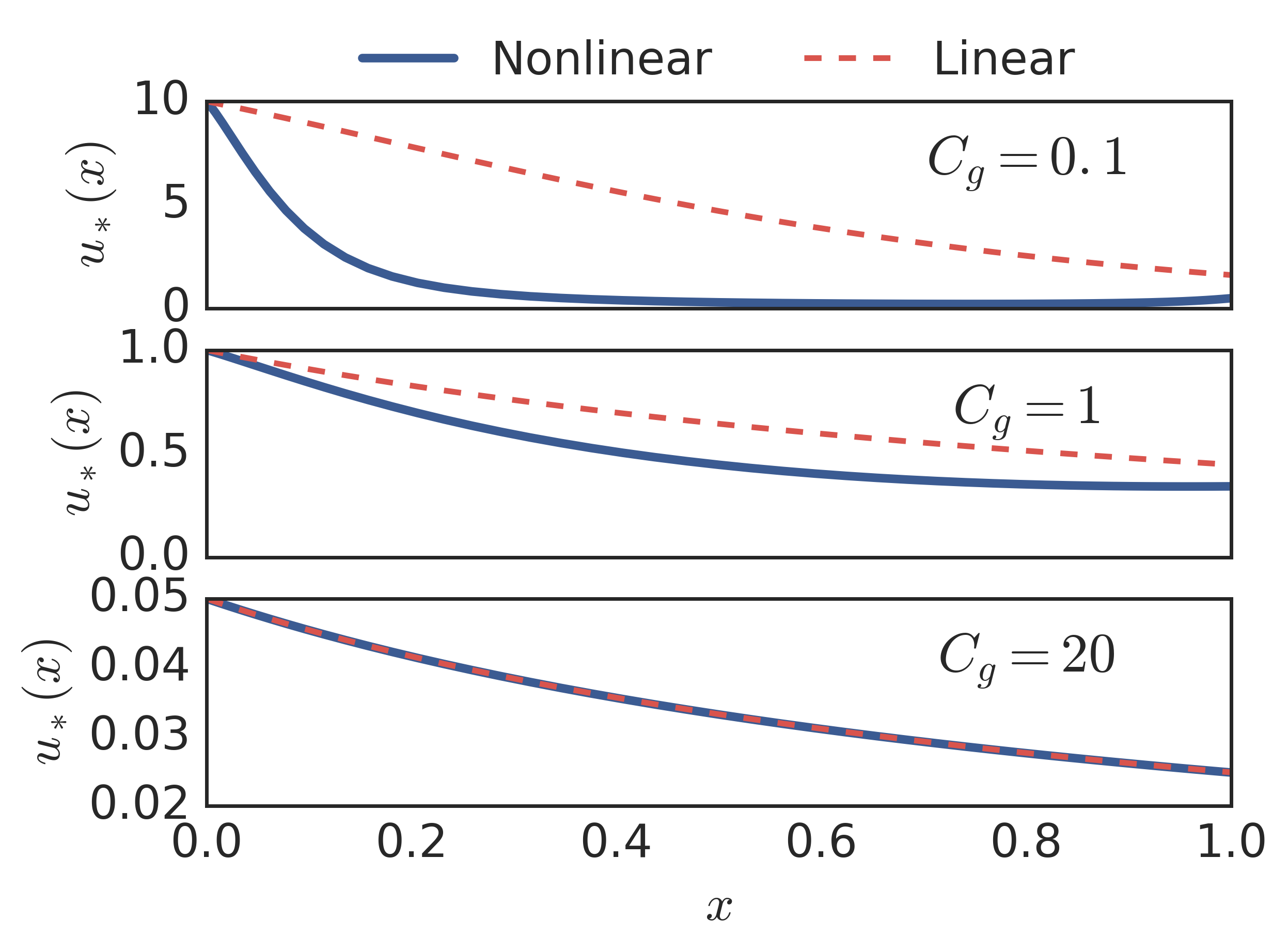
(a)

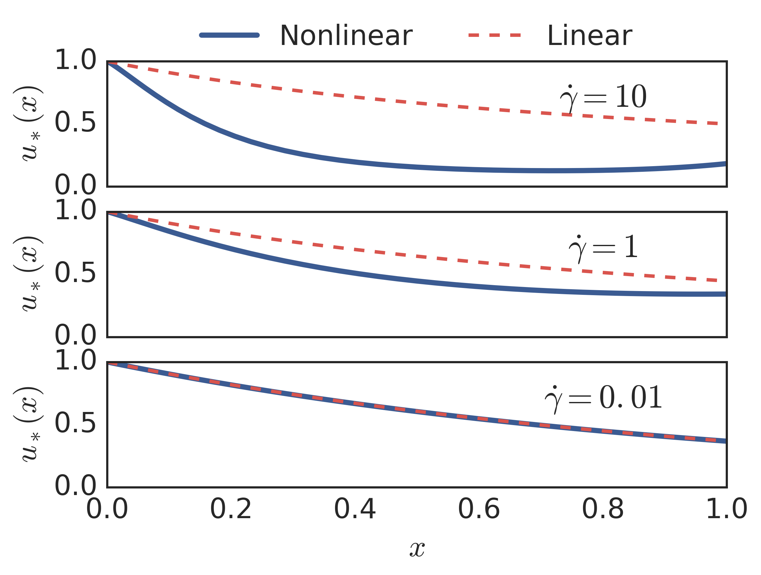
(b)

Figure 2: Results of some numerical simulations. Dashed red and solid blue lines correspond to the stationary of the linear Sinko-Streifer and the nonlinear microbial flocculation equations, respectively. a) Steady state solutions for increasing growth rate b) Steady state solutions for decreasing shear rate

Stationary solutions of the linear and nonlinear case for several different values of $C_{g}$ are depicted in Figure 2a. It is interesting to note that for increasing values of $C_{g}$ the growth dominates and thus stationary solution of the nonlinear case approaches the stationary solutions of the linear case. Analogously, as one could expect, results in Figure 2b indicate that as $\dot{\gamma}\to 0$ the stationary solutions of the microbial flocculation model converge to that of essentially linear Sinko-Streifer model.

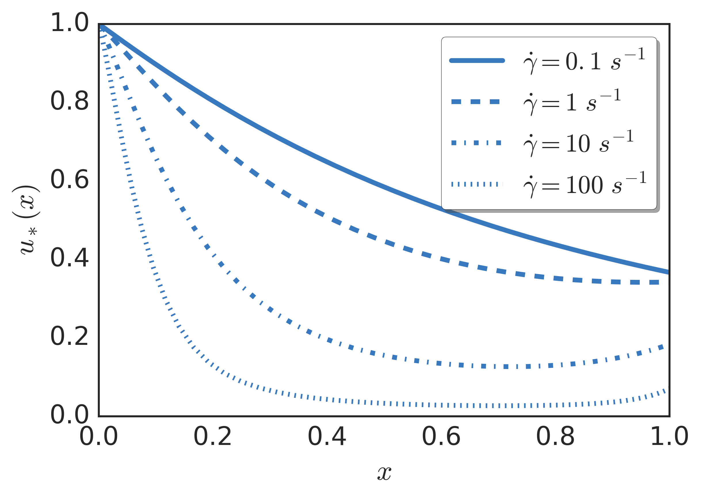
(a)

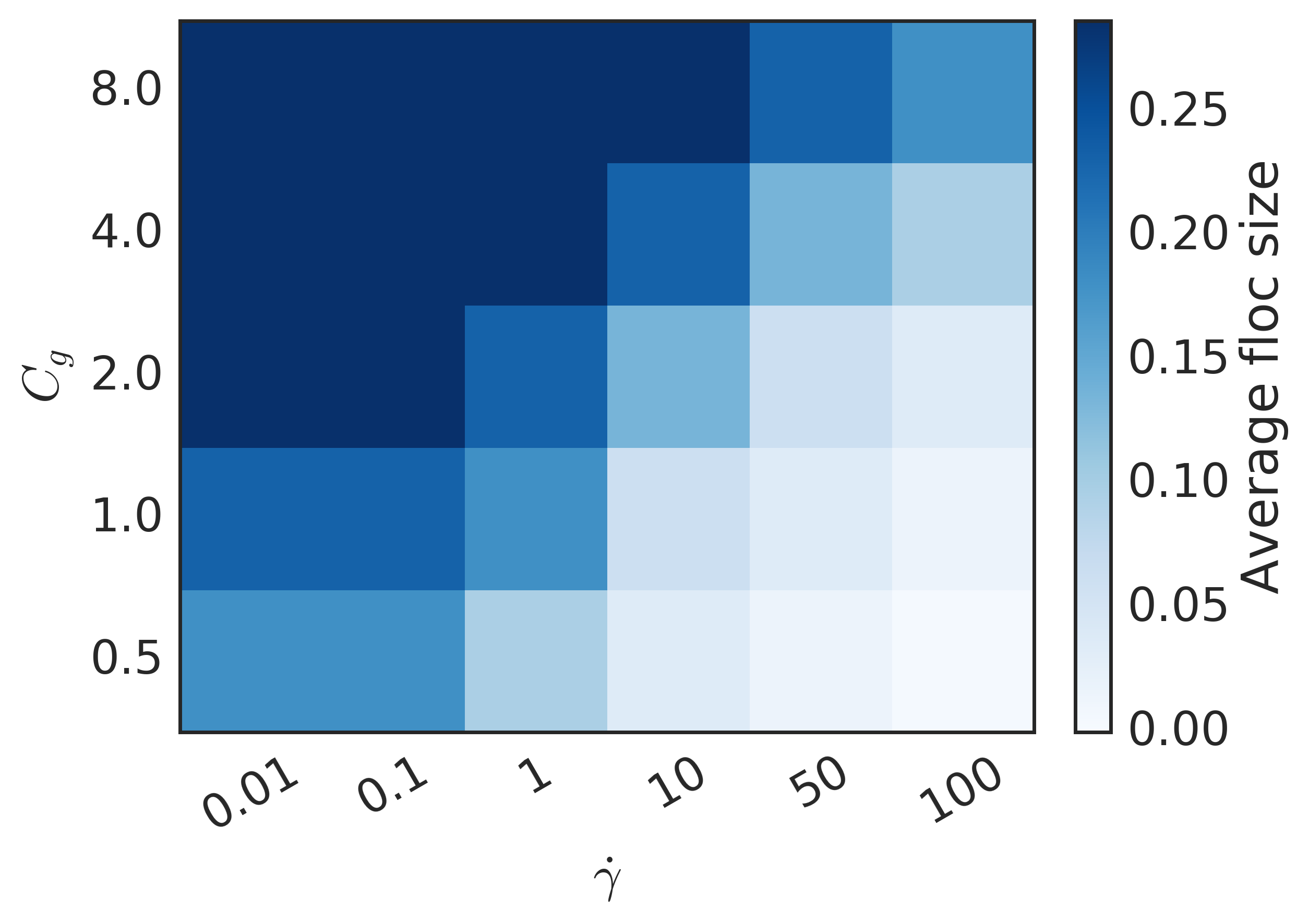
(b)

Figure 3: Effect of the shear rate on the average floc size and the renewal rate. a) Increasing the shear rate results in stationary distributions with smaller average floc size. b) For each given growth rate of a microbial floc, increasing the shear rate decreases the average floc size.

Thorough control of floc formation is crucial for proper operation of bioreactors used in fermentation industry and waste water treatment. For efficient removal of suspended particles, it is usually desirable to have larger and denser flocs that settle faster under gravitational forces. Therefore, in Figures 3a and 3b, we investigated the effects of the shear rate on the average floc size. One can observe in Figure 3a that increasing the shear rate results in increased fragmentation of the flocs and thus drives the stationary distribution into the smaller size range, which is also consistent with the results of [18]. Moreover, results in Figure 3b indicate that for each given growth rate of a microbial floc one can adjust the shear rate to yield an optimal average floc size.

As it is stated in Theorem 2.1, for the existence of a positive stationary solution the renewal rate has to be modified according to equation (9). Consequently, in Figure 4a, for different growth and shear rates we computed the renewal rate $C_{q}$ based on the equation (21). Computed renewal rates lie on a smooth three-dimensional surface. Moreover, the results indicate that the renewal rate is directly proportional to both growth and shear rates.

The numerical algorithm described in this chapter can be easily modified to find steady states of the boundary value problem in (15). In this general case, the results of Section 2 do not guarantee the existence of a positive steady state. However, Figure 4b depicts that positive steady states exist for the points not lying on the surface illustrated in Figure 4a. This in turn suggests well-posedness of the boundary value problem given in (15) for sufficiently smooth model rates. Therefore, as the future plan, we wish to further investigate well-posedness of this boundary value problem.

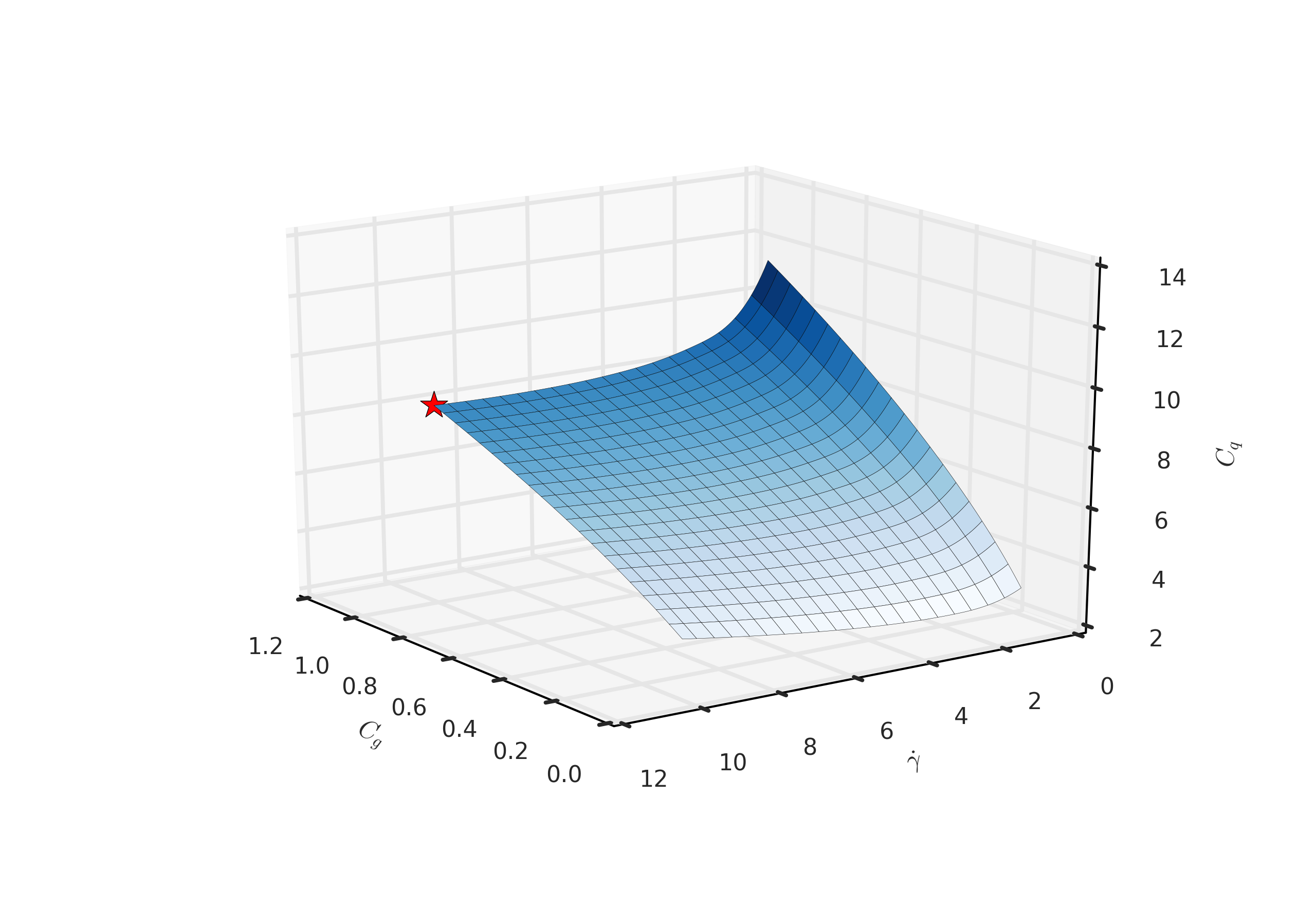
(a)

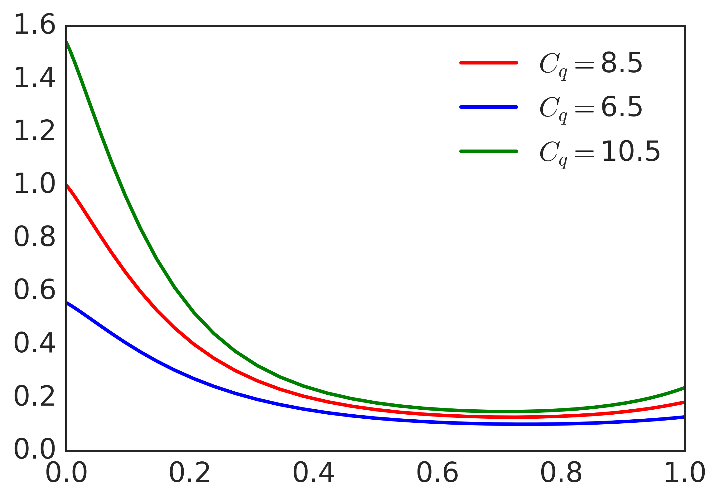
(b)

Figure 4: Effect of growth and shear rates on the renewal rate, $C_{q}$. a) Renewal rates form a smooth surface. Marked red star corresponds to the point $C_{g}=1$, $\dot{\gamma}=1$ and $C_{q}=8.5$ b) Steady states for marked red star and some points below and above the marked point.

5 Concluding remarks

Our primary motivation in this paper is to investigate the ultimate behavior of solutions of a generalized size-structured flocculation model. The model accounts for a broad range of biological phenomena (necessary for survival of a community of microorganism in a suspension) including growth, aggregation, fragmentation, removal due to predation, and gravitational sedimentation. Moreover, the number of cells that erode from a floc and enter the single cell population is modeled with McKendrick-von Foerster type renewal boundary equation. Although it has been shown that the model has a unique positive solution, to the best of our knowledge, the large time behavior of those solutions has not been studied. Therefore, in this paper we showed that under relatively weak restrictions the flocculation model possesses a non-trivial stationary solution (in addition to the trivial stationary solution).

We developed a numerical scheme based on spectral collocation method to approximate these nontrivial stationary solutions. Our numerical exploration of the stationary solutions of the microbial flocculation model indicate that for sufficiently large growth rates the stationary solutions converge to stationary solutions of the linear Sinko-Streifer model (2). Therefore, as future research, we plan to study this behavior analytically.

Furthermore, in Section 4, we numerically investigated physically relevant parameter ranges. In particular, we studied the effects of the shear rate on the average floc size. Our results (consistent with the result in the literature [18, 42, 40]) indicate that increasing the shear rate of the stirring tank results in increased fragmentation, and thus decreasing the steady-state average floc size.

References

- Ackleh, [1997] Ackleh, A. S. (1997). Parameter estimation in a structured algal coagulation-fragmentation model. Nonlinear Analysis, 28(5):837–854.
- Ackleh and Fitzpatrick, [1997] Ackleh, A. S. and Fitzpatrick, B. G. (1997). Modeling aggregation and growth processes in an algal population model: analysis and computations. J. Math. Biol., 35(4):480–502.
- Aldous, [1999] Aldous, D. J. (1999). Deterministic and Stochastic Models for Coalescence (Aggregation, Coagulation): A Review of the Mean-Field Theory for Probabilists. Bernoulli, 5(1):3–48.
- Banasiak, [2011] Banasiak, J. (2011). Blow-up of solutions to some coagulation and fragmentation equations with growth. Discrete and Continuous Dynamical Systems, pages 126–134.
- Banasiak and Lamb, [2009] Banasiak, J. and Lamb, W. (2009). Coagulation, fragmentation and growth processes in a size structured population. Discrete Contin. Dyn. Syst. - Ser. B, 11(3):563–585.
- Bortz, [2015] Bortz, D. M. (2015). Chapter 17: Modeling and simulation for nanomaterials in fluids: Nanoparticle self-assembly. In Tewary, V. and Zhang, Y., editors, Modeling, characterization, and production of nanomaterials: Electronics, Photonics and Energy Applications, volume 73 of Woodhead Publishing Series in Electronic and Optical Materials, pages 419–441. Woodhead Publishing Ltd., Cambridge, UK.
- Bortz et al., [2008] Bortz, D. M., Jackson, T. L., Taylor, K. A., Thompson, A. P., and Younger, J. G. (2008). Klebsiella pneumoniae Flocculation Dynamics. Bull. Math. Biol., 70(3):745–768.
- Byrne et al., [2011] Byrne, E., Dzul, S., Solomon, M., Younger, J., and Bortz, D. M. (2011). Postfragmentation density function for bacterial aggregates in laminar flow. Phys. Rev. E, 83(4).
- Calvez et al., [2012] Calvez, V., Doumic, M., and Gabriel, P. (2012). Self-similarity in a general aggregation–fragmentation problem. Application to fitness analysis. Journal de Mathématiques Pures et Appliquées, 98(1):1–27.
- Calvez et al., [2010] Calvez, V., Lenuzza, N., Doumic, M., Deslys, J.-P., Mouthon, F., and Perthame, B. (2010). Prion dynamics with size dependency–strain phenomena. J. Biol. Dyn., 4(1):28–42.
- Doumic-Jauffret and Gabriel, [2009] Doumic-Jauffret, M. and Gabriel, P. (2009). Eigenelements of a General Aggregation-Fragmentation Model. ArXiv09075467 Math.
- Dubovskii, [1994] Dubovskii, P. B. (1994). Mathematical Theory of Coagulation. Number 23 in Lecture Notes Series. Seoul National University, Research Institute of Mathematics, Global Analysis Research Center, Seoul National University, Seoul 151-742, Korea.
- Dubovskii and Stewart, [1996] Dubovskii, P. B. and Stewart, I. W. (1996). Existence, Uniqueness and Mass Conservation for the Coagulation-Fragmentation Equation. Mathematical Methods in the Applied Sciences, 19(7):571–591.
- Ducoste, [2002] Ducoste, J. (2002). A two-scale PBM for modeling turbulent flocculation in water treatment processes. Chemical Engineering Science, 57(12):2157–2168.
- Escobedo et al., [2002] Escobedo, M., Mischler, S., and Perthame, B. (2002). Gelation in Coagulation and Fragmentation Models. Communications in Mathematical Physics, 231(1):157–188.
- Farkas and Hagen, [2007] Farkas, J. Z. and Hagen, T. (2007). Stability and regularity results for a size-structured population model. J. Math. Anal. Appl., 328(1):119–136.
- Farkas and Hinow, [2012] Farkas, J. Z. and Hinow, P. (2012). Steady states in hierarchical structured populations with distributed states at birth. Discrete Contin. Dyn. Syst. - Ser. B, 17(8):2671–2689.
- Flesch et al., [1999] Flesch, J. C., Spicer, P. T., and Pratsinis, S. E. (1999). Laminar and turbulent shear-induced flocculation of fractal aggregates. AIChE Journal, 45:1114–1124.
- Fornberg, [1998] Fornberg, B. (1998). A Practical Guide to Pseudospectral Methods. Cambridge University Press.
- Fournier and Laurençot, [2005] Fournier, N. and Laurençot, P. (2005). Existence of self-similar solutions to Smoluchowski’s coagulation equation. Communications in Mathematical Physics, 256(3):589–609.
- Jewett and Serway, [2008] Jewett, J. W. and Serway, R. A. (2008). Physics for Scientists and Engineers with Modern Physics. Cengage Learning EMEA.
- Kightley et al., [2018] Kightley, E. P., Pearson, A., Evans, J. A., and Bortz, D. M. (2018). Fragmentation of biofilm-seeded bacterial aggregates in shear flow. European Journal of Applied Mathematics, (accepted).
- Laurençot and Walker, [2005] Laurençot, P. and Walker, C. (2005). Steady States for a Coagulation-Fragmentation Equation with Volume Scattering.
- Laurencot and Walker, [2005] Laurencot, P. and Walker, C. (2005). Steady States for a Coagulation-Fragmentation Equation with Volume Scattering. SIAM Journal on Mathematical Analysis. doi:10.1137/S0036141004444111.
- Li et al., [2004] Li, X.-y., Zhang, J.-j., and Lee, J. H. W. (2004). Modelling particle size distribution dynamics in marine waters. Water Research, 38(5):1305–1317.
- Makino et al., [1998] Makino, J., Fukushige, T., Funato, Y., and Kokubo, E. (1998). On the mass distribution of planetesimals in the early runaway stage. New Astronomy, 3(7):411–417.
- Matveev et al., [2015] Matveev, S. A., Smirnov, A. P., and Tyrtyshnikov, E. E. (2015). A fast numerical method for the Cauchy problem for the Smoluchowski equation. Journal of Computational Physics, 282:23–32.
- Menon and Pego, [2005] Menon, G. and Pego, R. L. (2005). Dynamical Scaling in Smoluchowski’s Coagulation Equations: Uniform Convergence. SIAM Journal on Mathematical Analysis, 36(5):1629.
- Menon and Pego, [2006] Menon, G. and Pego, R. L. (2006). Dynamical Scaling in Smoluchowski’s Coagulation Equations: Uniform Convergence. SIAM Review, 48(4):745.
- Mirzaev and Bortz, [2017] Mirzaev, I. and Bortz, D. M. (2017). A numerical framework for computing steady states of structured population models and their stability. Mathematical Biosciences and Engineering, 14(4):1–20.
- Mirzaev et al., [2016] Mirzaev, I., Byrne, E. C., and Bortz, D. M. (2016). An Inverse Problem for a Class of Conditional Probability Measure-Dependent Evolution Equations. Inverse Problems, 32(9):095005.
- Nicmanis and Hounslow, [1998] Nicmanis, M. and Hounslow, M. J. (1998). Finite-element methods for steady-state population balance equations. AIChE J., 44(10):2258–2272.
- Niwa, [1998] Niwa, H.-S. (1998). School Size Statistics of Fish. J. Theor. Biol., 195(3):351–361.
- Piani et al., [2014] Piani, L., Rizzardini, C. B., Papo, A., and Goi, D. (2014). Rheology Measurements for Online Monitoring of Solids in Activated Sludge Reactors of Municipal Wastewater Treatment Plant. ScientificWorldJournal, 2014.
- Pruppacher and Klett, [2012] Pruppacher, H. R. and Klett, J. D. (2012). Microphysics of Clouds and Precipitation: Reprinted 1980. Springer Science & Business Media.
- Prüss, [1983] Prüss, J. (1983). On the qualitative behaviour of populations with age-specific interactions. Computers & Mathematics with Applications, 9(3):327–339.
- Saffman and Turner, [1956] Saffman, P. G. and Turner, J. S. (1956). On the collision of drops in turbulent clouds. Journal of Fluid Mechanics, 1(01):16–30.
- Sinko and Streifer, [1967] Sinko, J. W. and Streifer, W. (1967). A New Model For Age-Size Structure of a Population. Ecology, 48(6):910–918.
- Spicer, [1995] Spicer, P. T. (1995). Shear-Induced Aggregation-Fragmentation: Mixing and Aggregate Morphology Effects. PhD thesis, University of Cincinnati.
- Spicer, [1997] Spicer, P. T. (1997). Shear-Induced Aggregation- Fragmentation : Mixing and Aggregate Morphology Effects by. PHD Thesis, page 283.
- Spicer and Pratsinis, [1996] Spicer, P. T. and Pratsinis, S. E. (1996). Coagulation and fragmentation: Universal steady-state particle-size distribution. AIChE journal, 42(6):1612–1620.
- Spicer et al., [1998] Spicer, P. T., Pratsinis, S. E., Raper, J., Amal, R., Bushell, G., and Meesters, G. (1998). Effect of shear schedule on particle size, density, and structure during flocculation in stirred tanks. Powder Technology, 97(1):26–34.
- Spicer et al., [1996] Spicer, P. T., Pratsinis, S. E., Trennepohl, M. D., and Meesters, G. H. M. (1996). Coagulation and Fragmentation: The Variation of Shear Rate and the Time Lag for Attainment of Steady State. Industrial & Engineering Chemistry Research, 35(9):3074–3080.
- Trefethen, [2000] Trefethen, L. (2000). Spectral Methods in MATLAB. Software, Environments and Tools. Society for Industrial and Applied Mathematics.
- van Smoluchowski, [1917] van Smoluchowski, M. (1917). Versuch einer mathematischen theorie der koagulation kinetic kolloider losungen. Zeitschrift f{ü}r physikalische Chemie, 92:129–168.
- Wattis, [2006] Wattis, J. A. D. (2006). An introduction to mathematical models of coagulation-fragmentation processes: A discrete deterministic mean-field approach.
- Ziff and Stell, [1980] Ziff, R. M. and Stell, G. (1980). Kinetics of polymer gelation. J. Chem. Phys., 73(7):3492–3499.