3 April 2018, revised 31 May 2018

Elastic Compton Scattering from ${}^{3}\text{He}$
and the Role of the Delta

Arman Margaryan^a Bruno Strandberg^b,c Harald W. Grießhammer^d,

Judith A. McGovern^e Daniel R. Phillips^f and Deepshikha Shukla^g

^aL/EFT Group, Department of Physics,
Duke University, Box 90305, Durham, NC 27708, USA
^bSchool of Physics and Astronomy, University of Glasgow,
Glasgow G12 8QQ, Scotland, UK
^cNikhef, Science Park 105, 1098 XG Amsterdam, Netherlands
^dInstitute for Nuclear Studies, Department of Physics,
The George Washington University, Washington DC 20052, USA
^eSchool of Physics and Astronomy, The University of Manchester,
Manchester M13 9PL, UK
^fDepartment of Physics and Astronomy and Institute of Nuclear and Particle Physics, Ohio University, Athens, OH 45701, USA
^gDepartment of Mathematics, Computer Science and Physics,
Rockford University, Rockford, IL 61108, USA

We report observables for elastic Compton scattering from ${}^{3}\text{He}$ in Chiral Effective Field Theory with an explicit $\Delta(1232)$ degree of freedom ($\chi$EFT) for energies between $50$ and $120\;\mathrm{MeV}$. The $\gamma\,$${}^{3}\text{He}$ amplitude is complete at N³LO, $\mathcal{O}(\mathrm{e}^{2}\delta^{3})$, and in general converges well order by order. It includes the dominant pion-loop and two-body currents, as well as the Delta excitation in the single-nucleon amplitude. Since the cross section is two to three times that for deuterium and the spin of polarised ${}^{3}\text{He}$ is predominantly carried by its constituent neutron, elastic Compton scattering promises information on both the scalar and spin polarisabilities of the neutron. We study in detail the sensitivities of $4$ observables to the neutron polarisabilities: the cross section, the beam asymmetry and two double asymmetries resulting from circularly polarised photons and a longitudinally or transversely polarised target. Including the Delta enhances those asymmetries from which neutron spin polarisabilities could be extracted. We also correct previous, erroneous results at N²LO, i.e. without an explicit Delta, and compare to the same observables on proton, neutron and deuterium targets. An interactive Mathematica notebook of our results is available from hgrie@gwu.edu.

Suggested Keywords: Compton scattering, Helium-3, Effective Field Theory, neutron polarisabilities, spin polarisabilities, $\Delta(1232)$ resonance

1 Introduction

Elastic Compton scattering from a Helium-3 target has been identified as a promising means to access neutron electromagnetic polarisabilities. In refs. [1, 2, 3, 4], Shukla et al. showed that the differential cross section in the energy range of $50$ to $120\;\mathrm{MeV}$ is sensitive to the electric and magnetic dipole polarisabilities of the neutron, $\alpha_{E1}^{(\mathrm{n})}$ and $\beta_{M1}^{(\mathrm{n})}$, and that scattering on polarised ${}^{3}\text{He}$ provides good sensitivity to the neutron spin polarisabilities. These calculations were carried out at ${\cal O}(Q^{3})$ in the Chiral Effective Field Theory expansion and led to proposals at MAMI and HI$\gamma$S to exploit this opportunity to extract neutron polarisabilities from elastic $\gamma\,$${}^{3}\text{He}$ scattering [5, 6, 7, 8, 9].

Here, we extend the calculation of refs. [1, 2, 3] by one order in the chiral counting by incorporating the leading effects of the $\Delta(1232)$. As discussed in an erratum published simultaneously with this paper [4], these first results were obtained from a computer code which contained mistakes, and we take the opportunity to correct some of the results here as well.

$\chi$EFT is the low-energy Effective Field Theory of QCD; see, e.g., refs. [10, 11, 12] for reviews of the mesonic and one-nucleon sector, and refs. [13, 14, 15] for summaries of the few-nucleon sector. It respects the spontaneously and dynamically broken $\mathrm{SU}(2)_{L}\times\mathrm{SU}(2)_{R}$ symmetry of QCD and has nucleons and pions as explicit degrees of freedom. In this work, we consider a variant which also includes the Delta [16, 17, 18, 19]. Since $\chi$EFT provides a perturbative expansion of observables in a small, dimension-less parameter, one can calculate observables to a given order, which in turns provides a way to estimate the residual theoretical uncertainties from the truncation [20, 21].

More details on the $\chi$EFT expansion are given in sect. 2.1; for now, we summarise our calculation as follows. We employ both the $\gamma N$ and $\gamma NN$ amplitudes of refs. [22, 10, 23] and supplement those with the $\Delta$-pole and $\pi\Delta$ loop graphs [24, 25, 26, 27]. The different pieces of the photonuclear operator are organised in a perturbative expansion which is complete to N³LO [${\cal O}(e^{2}\delta^{3})$]. Hence, it includes not only the Thomson term for the protons, as well as magnetic moment couplings and dynamical single-nucleon effects such as virtual pion loops and the Delta excitation, but also significant contributions from the coupling of external photons to the charged pions that are exchanged between neutrons and protons (referred to hereafter as “two-nucleon/two-body currents”). The photonuclear operator is evaluated between ${}^{3}\text{He}$ wave functions, which are calculated from $NN$ and $3N$ potentials derived using the same perturbative $\chi$EFT expansion [28, 29, 30].

While $\gamma{}^{3}\text{He}$ experiments are only in the planning stages [5, 6, 7, 8, 9], the past two decades have seen significant progress in measurements of Compton scattering on the deuteron. However, deuteron data only provides access to the isoscalar polarisabilities; a ${}^{3}\text{He}$ target provides complementary information on neutron polarisabilities. A naïve model of the ${}^{3}\text{He}$ nucleus as two protons paired with total spin zero plus a neutron suggests that observables should depend on the combinations $2\alpha_{E1}^{(\mathrm{p})}+\alpha_{E1}^{(\mathrm{n})}$, $2\beta_{M1}^{(\mathrm{p})}+\beta_{M1}^{(\mathrm{n})}$, and that dependence on proton spin polarisabilities should be minimal. Such a picture is somewhat over-simplified; see sect. 5. Still, relative to the deuteron, ${}^{3}\text{He}$ data offers the promise of stronger signals and of cross-validation of the theory used to subtract binding effects and extract nucleon polarisabilities.

Most recently, Myers et al. [31, 32] measured the differential cross section on the deuteron at energies ranging from $65$ to $115\;\mathrm{MeV}$, doubling the world data for elastic $\gamma d$ scattering. In combination with the proton results quoted below, a fit using the $\chi$EFT $\gamma d$ amplitude at the same order, ${\cal O}(e^{2}\delta^{3})$, as the current work, yields

$$\begin{split}\alpha_{E1}^{(\mathrm{n})}&=11.55\pm 1.25\mathrm{(stat.)}\pm 0.2\mathrm{(Baldin)}\pm 0.8\mathrm{(theory)}\;\;,\\ \beta_{M1}^{(\mathrm{n})}&=3.65\mp 1.25\mathrm{(stat.)}\pm 0.2\mathrm{(Baldin)}\mp 0.8\mathrm{(theory)}\end{split}$$ (1.1)

for the electric and magnetic dipole polarisabilities of the neutron. The canonical units of $10^{-4}\leavevmode\nobreak\ \mathrm{fm}^{3}$ are employed. Here, the Baldin sum rule $\alpha_{E1}^{(\mathrm{n})}+\beta_{M1}^{(\mathrm{n})}=15.2\pm 0.4$ [33, 34] was used as a constraint, and the third error listed is an estimate of the theory uncertainty. Equation (1.1) is consistent with the extraction of neutron polarisabilities from quasi-free Compton scattering on the neutron in deuterium [35, 36, 37]. Further refinement of extractions from deuterium data is expected thanks to ongoing experiments at HI$\gamma$S [5, 7, 8, 38] and the ongoing extension of the $\chi$EFT calculation to $\mathcal{O}(e^{2}\delta^{4})$ [39]. A comprehensive review of experimental and $\chi$EFT work on Compton scattering from deuterium can be found in ref. [40], which also summarises work on the proton in $\chi$EFT.

Concurrently, refs. [41, 21] extracted the electric dipole polarisabilities of the proton using the data set of $\gamma p$ elastic differential cross section data compiled in ref. [40] and the $\mathcal{O}(e^{2}\delta^{4})$ $\chi$EFT $\gamma p$ amplitude:

$$\begin{split}\alpha_{E1}^{(\mathrm{p})}&=10.65\pm 0.35(\text{stat})\pm 0.2(\text{Baldin})\pm 0.3(\text{theory})\;,\\ \beta_{M1}^{(\mathrm{p})}&=\phantom{0}3.15\mp 0.35(\text{stat})\pm 0.2(\text{Baldin})\mp 0.3(\text{theory})\;\;.\end{split}$$ (1.2)

Here, the Baldin sum rule value $\alpha_{E1}^{(\mathrm{p})}+\beta_{M1}^{(\mathrm{p})}=13.8\pm 0.4$ was used. It is fully consistent with a more recent determination of $\alpha_{E1}^{(\mathrm{p})}+\beta_{M1}^{(\mathrm{p})}=14.0\pm 0.2$ [42]. Compared to the neutron values, the uncertainties are much smaller, for two reasons. The proton extraction used the $\chi$EFT $\gamma p$ amplitude at $\mathcal{O}(e^{2}\delta^{4})$, i.e. at one order higher than the deuteron extraction, leading to smaller theoretical uncertainties. The main difference is however that the deuteron data set is of lesser quality than that of the proton, contains fewer points, and is restricted to a much smaller energy range. This results in statistical uncertainties which are nearly four times those of the proton. Therefore, these extractions provide only a hint that the proton and neutron polarisabilities may be different. Reducing the experimental error bars is imperative to conclude whether short-range effects lead to small proton-neutron differences; such differences would have potentially important implications for the proton-neutron mass splitting, see, e.g., ref. [21] and references therein. We argue that Compton scattering on ${}^{3}\text{He}$ can serve to improve the neutron values.

In addition to the scalar polarisabilities, four spin polarisabilities $\gamma_{E1E1}$, $\gamma_{M1M1}$, $\gamma_{E1M2}$ and $\gamma_{M1E2}$ parametrise the response of the nucleon’s spin degrees of freedom to electromagnetic fields of particular multipolarities. Intuitively interpreted, the electromagnetic field of the spin degrees causes bi-refringence in the nucleon, just as in the classical Faraday-effect [43]. The type of experiment that will be most sensitive to the spin polarisabilities involves polarised photons and targets. A comprehensive exploration of such sensitivities for the proton was recently published by some of the current authors [44]. Some data exist, and in Ref. [45] it was used to fit a subset of the spin polarisabilities. The values obtained agree well within the respective uncertainties with $\chi$EFT predictions [21]. However, it was argued in Ref. [44] that much of the data is at energies that are too high for any extraction to be independent of the theoretical framework employed.

No experiments have yet probed the individual neutron spin polarisabilities, which are also predicted by $\chi$EFT at the same order [21]. They can be measured with a polarised deuteron target [46, 47, 48, 49], but that has not yet been attempted. Refs. [1, 2, 3] identified polarised ${}^{3}\text{He}$ as a promising candidate because the dominant ($\approx 95$%) wave function component in ${}^{3}\text{He}$ consists of two protons in a spin-singlet pair. The spin of the nucleus is then carried by the neutron and observables are about $20$ times more sensitive to neutron spin polarisabilities than to their proton counterparts. Indeed, we will confirm again in sects. 4.5 and 4.6 that $\chi$EFT predicts only small corrections to this expectation, which are slightly different for each observable and both energy- and angle-dependent. Even if Compton scattering from a free neutron were feasible, cross sections for coherent Compton scattering from ${}^{3}\text{He}$ are markedly larger than those for on a (quasi-)free neutron in this energy range. This is because in ${}^{3}\text{He}$, the neutron contributions interfere with the proton ones and with those from two-body currents; see sect. 5 for comparisons to proton, neutron and deuteron targets.

In this presentation, we therefore examine the influence of the Delta on the cross section and asymmetries, using the same photonuclear kernel as in the extraction of the scalar polarisabilities of the neutron from $\gamma$d data, eq. (1.1) [40, 31, 32]. The Delta degree of freedom plays a significant role in some of the spin polarisabilities, especially in $\gamma_{M1M1}$. In $\gamma d$ scattering, its inclusion markedly enhances the pertinent asymmetries [47, 48, 49]. It is therefore important to examine its impact on the ${}^{3}\text{He}$ asymmetries.

All observables presented are available via a Mathematica notebook from hgrie@gwu.edu. It contains results for cross sections, rates and asymmetries from $50$ to about $120$ MeV in the lab frame, and allows the scalar and spin polarisabilities to be varied, including variations constrained by sum rules.

This article is organised as follows. In sect. 2, we summarise the ${\cal O}(e^{2}\delta^{3})$ amplitude that constitutes the Compton-scattering operator in our calculation and sketch details of computing matrix elements of that operator between ${}^{3}\text{He}$ wave functions. Section 3 then defines the different observables, before sect. 4 presents the results of our study. Section 5 offers a summary and comparisons of $\chi$EFT predictions for Compton scattering on the proton, neutron, deuteron, and ${}^{3}\text{He}$.

2 ${}^{3}\text{He}$ Compton Scattering in $\chi$EFT with the Delta

2.1 Chiral Effective Field Theory

Compton scattering on nucleons and light nuclei in $\chi$EFT has been reviewed in refs. [40, 41], to which we refer the reader for notation, relevant parts of the chiral Lagrangian, and full references to the literature. Here, we first briefly summarise the power counting; then we sketch the content of the $\mathcal{O}(e^{2}\delta^{3})$ amplitude for Compton scattering on ${}^{3}\text{He}$, which at this order only consists of one- and two-nucleon contributions to a photonuclear kernel evaluated between nuclear wave functions.

In $\chi$EFT with a dynamical Delta, Compton scattering exhibits three low-momentum scales: the pion mass $m_{\pi}$, the Delta-nucleon mass splitting $\Delta_{\scriptscriptstyle M}\approx 300\;\mathrm{MeV}$, and the photon energy $\omega$. Each provides a small, dimensionless expansion parameter when it is measured in units of the “high” scale $\Lambda_{\chi}$ at which the theory breaks down because new degrees of freedom enter.

While the two ratios $\frac{m_{\pi}}{\Lambda_{\chi}}$ and $\frac{\Delta_{\scriptscriptstyle M}}{\Lambda_{\chi}}$ have very different chiral behaviour, we follow Pascalutsa and Phillips [19] and take a common breakdown scale $\Lambda_{\chi}\approx 650\;\mathrm{MeV}$, which is consistent with the masses of the $\omega$ and $\rho$ as the next-lightest exchange mesons, and then exploit a numerical coincidence for the physical pion masses to define a single expansion parameter:

$$\delta\equiv\frac{\Delta_{M}}{\Lambda_{\chi}}\approx\left(\frac{m_{\pi}}{\Lambda_{\chi}}\right)^{1/2}\approx 0.4\ll 1\;\;.$$ (2.1)

We also count $M_{\mathrm{N}}\sim\Lambda_{\chi}$. Since $\delta$ is not very small, order-by-order convergence must be verified carefully; see our discussion for each observable in sect. 4.

The treatment of the scale $\omega$ depends on the experiment [40, 41]. In this paper, we concentrate on energies for which $\omega\lesssim m_{\pi}\sim\delta^{2}\Lambda_{\chi}\ll\Delta_{M}$ counts like a chiral scale and pion-cloud physics therefore dominates. As reviewed below, pion-cloud effects enter at $\mathcal{O}(e^{2}\delta^{2})$ [N²LO], while the Delta appears at $\mathcal{O}(e^{2}\delta^{3})$ [N³LO]. Including it is simply equivalent to adding one order. We note that the version of $\chi$EFT without a dynamical Delta (often called Heavy Baryon Chiral Perturbation Theory) is limited to momenta well below the resonance. We denote its expansion parameter by $Q$, and its N²LO is identical to ours, $\mathcal{O}(Q^{3})\equiv\mathcal{O}(e^{2}\delta^{2})$; see ref. [40, sect. 4.2.7] for more details. The counting changes at both higher photon energies, where $\omega\sim\Delta_{M}$, and also at lower energies, where $\omega\sim m_{\pi}^{2}/M_{\mathrm{N}}$ is comparable to the typical nuclear binding momentum. The latter limit is more relevant to the current paper, since, as we will see in sect. 2.4.2, it sets a lower limit on the energy for which our calculations may be considered reliable. In particular, calculations consistent with the low-energy counting are required to have the correct nuclear Thomson limit; the current calculation would overshoot considerably as $\omega\to 0$. We will address both extensions to higher and lower energies in future publications [50].

Our focus is therefore on energies in the overlap of the single-nucleon regime (i) of refs. [40, 41] and the few-nucleon regime (II) of ref. [40] : $50\;\mathrm{MeV}\lesssim\omega\lesssim 120\;\mathrm{MeV}$.

2.2 Compton Kernel: Single-Nucleon Contributions

Contributions to the single-nucleon amplitude up to $\mathcal{O}(e^{2}\delta^{3})$ or N³LO in the regime $50\;\mathrm{MeV}\lesssim\omega\lesssim 120\;\mathrm{MeV}$ are sketched in fig. 1:

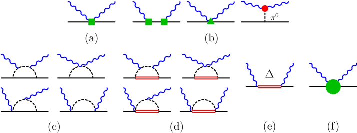
Figure 1: (Colour on-line) The single-nucleon contributions in $\chi$EFT up to $\mathcal{O}(e^{2}\delta^{3})$ for $50\;\mathrm{MeV}\lesssim\omega\lesssim 120\;\mathrm{MeV}$. The vertices are from: ${\cal L}_{\pi\mathrm{N}}^{(1)}$ (no symbol), ${\cal L}_{\pi\mathrm{N}}^{(2)}$ (green square), ${\cal L}_{\pi\mathrm{N}}^{(3)}$ (green triangle), ${\cal L}_{\pi\pi}^{(4)}$ (red disc) [10]; the green disc of graph (f) stands for variations of the polarisabilities, cf. eq. (4.3). Permuted and crossed diagrams are not displayed.

• LO [$\mathcal{O}(e^{2}\delta^{0}=Q^{2})$]: The single-nucleon (proton) Thomson term.

• N²LO [$\mathcal{O}(e^{2}\delta^{2}=Q^{3})$] non-structure/Born terms: photon couplings to the nucleon charge beyond LO, to its magnetic moment, or to the $t$-channel exchange of a $\pi^{0}$ meson. $\gamma\,$${}^{3}\text{He}$ scattering is sensitive to the latter, in contradistinction to $\gamma d$ scattering, where its expectation value is zero, as the deuteron is isoscalar.

• N²LO [$\mathcal{O}(e^{2}\delta^{2}=Q^{3})$] structure/non-Born terms: photon couplings to the pion cloud around the nucleon, the source of the LO contributions to the polarisabilities as first reported in refs. [22, 10].

• N³LO [$\mathcal{O}(e^{2}\delta^{3})$] structure/non-Born terms: photon couplings to the pion cloud around the Delta (d) or directly exciting the Delta (e), as calculated in refs. [51, 52]; these give NLO contributions to the polarisabilities. As detailed in ref. [40], we use a heavy-baryon propagator and a zero width, with $\Delta_{M}=293\;\mathrm{MeV}$, $g_{\pi\mathrm{N}\Delta}=1.425$. The non-relativistic version of the $N\Delta\gamma$ coupling is $b_{1}=5$ and tuned to give the same effective strength as the relativistic value of $g_{M}=2.9$ found by fitting to the proton data set up to the Delta resonance [40]. In practice, the $\pi\Delta$ loops produce almost-energy-independent contributions to $\alpha_{E1}$ and $\beta_{M1}$ for $\omega<200\;\mathrm{MeV}$.

• Short-distance/low-energy coefficients (LECs), which encode those contributions to the nucleon polarisabilities which stem from neither pion-cloud nor Delta effects; see eq. (4.3) for the precise form. These offsets to the polarisabilities are formally of higher order. For the proton, we fix these LECs to reproduce the $\mathcal{O}(e^{2}\delta^{2})$ values of the scalar polarisabilities. For the neutron, we exploit the freedom to vary the LECs in order to assess the sensitivity of cross sections and asymmetries to the neutron scalar polarisabilities. We refer to sect. 4.1 for the detailed procedure and values.

There is no contribution at NLO [$\mathcal{O}(e^{2}\delta^{1})$], and only Delta contributions at N³LO [$\mathcal{O}(e^{2}\delta^{3})$]. The difference between the previous $\mathcal{O}(e^{2}\delta^{2})$ [1, 2, 3] and our new $\mathcal{O}(e^{2}\delta^{3})$ calculation is hence the inclusion of Delta effects. Covariant kinematics for the fermion propagators, a nonzero Delta width, vertex corrections, etc. are just some examples of corrections which are of higher order than the last one we retain, N³LO [$\mathcal{O}(e^{2}\delta^{3})$]; they are parametrically small.

2.3 Compton Kernel: Two-Nucleon Contributions

The leading two-body currents in $\chi$EFT occur at $\mathcal{O}(e^{2}\delta^{2})$ and do not involve Delta excitations. They are the two-body analogue of the $\pi N$ loop graphs depicted in fig. 1 and thus denoted as $\mathcal{O}(Q^{3})$ in $\chi$EFT without dynamical Delta. They were first computed in ref. [23], where full expressions can be found. We depict them in fig. 2 below.

We note that the $\mathcal{O}(e^{2}\delta^{2})$ diagrams only contribute for $np$ pairs, i.e. they all contain an isospin factor of $\tau^{(1)}\cdot\tau^{(2)}-\tau^{(1)}_{z}\tau^{(2)}_{z}$. However, one distinction between ${}^{3}\text{He}$ and the deuteron is that in the tri-nucleon case both isospin zero and one pairs are present.

No corrections enter at the next order, $\mathcal{O}(e^{2}\delta^{3})$. Boost corrections and corrections with a nucleon propagating between the pion-exchange and a photon-nucleon interaction only enter at $\mathcal{O}(e^{2}\delta^{4})$ [23, 53, 40], and those with an intermediate Delta at $\mathcal{O}(e^{2}\delta^{5})$ [40]. Note that the pieces of the pion-exchange currents that are $1/M$ suppressed and must be derived consistently with the $NN$ potential [54, 55, 56] only enter at orders higher than we consider here; see discussion in sect. 2.4.2.

Figure 2: (Colour on-line) $\mathcal{O}(e^{2}\delta^{2})$ contributions to the (irreducible) $\gamma NN\rightarrow\gamma NN$ amplitude (no additional contributions at $\mathcal{O}(e^{2}\delta^{3})$). Notation as in fig. 1. Permuted and crossed diagrams not displayed.

2.4 From the Compton Kernel to Compton Amplitudes

Here, we provide a brief description of the computation of the integrals for ${}^{3}\text{He}$ matrix elements of the Compton operators in the centre-of-mass frame; full details can be found in refs. [3, 1].

2.4.1 Formulae for Matrix Elements

We seek a ${}^{3}\text{He}$-Compton amplitude which depends on the spin projections $M_{i/f}$ of the incoming and outgoing ${}^{3}\text{He}$ nucleus onto a common $z$ axis (which we define below to be the beam direction) and on the helicities $\lambda_{i/f}$ of the incident and outgoing photon. Using permutations and symmetries, this amplitude can be written as

$$A_{M_{i}\lambda_{i}}^{M_{f}\lambda_{f}}:=\langle M_{f},\lambda_{f}|T|M_{i},\lambda_{i}\rangle=3\,\langle M_{f}|\left(\frac{1}{2}\left[{\hat{O}}_{\lambda_{f}\lambda_{i}}^{1B}(1)+{\hat{O}}_{\lambda_{f}\lambda_{i}}^{1B}(2)\right]+{\hat{O}}_{\lambda_{f}\lambda_{i}}^{2B}(1,2)\right)|M_{i}\rangle\;,$$ (2.2)

where nucleons are numbered and $|M\rangle$ is an anti-symmetrised state of ${}^{3}\text{He}$. Since we are concerned with the ${}^{3}\text{He}$ nucleus, we also take this state to have isospin quantum numbers $T=M_{T}=1/2$. The operator ${\hat{O}}_{\lambda_{f}\lambda_{i}}^{1B}(a)$ with $a=1,\dots,3$ represents the one-body amplitude of sect. 2.2, where external photons of incoming (outgoing) helicity $\lambda_{i}$ ($\lambda_{f}$) interact with nucleon “$a$”. ${\hat{O}}_{\lambda_{f}\lambda_{i}}^{2B}(a,b)$ represents the corresponding two-body current of sect. 2.3, where the interaction is with the nucleon pair “$(a,b)$”. Thus in eq. (2.2), nucleon “$3$” serves as a spectator to the $\gamma NN\rightarrow\gamma NN$ scattering process. Three-nucleon currents (i.e. contributions of instantaneous interactions between three nucleons and at least one photon) do not enter before chiral order $e^{2}\delta^{6}$.

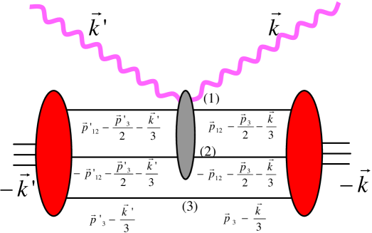
Figure 3: (Colour on-line) Kinematics of the calculation in the $\gamma$${}^{3}\text{He}$ centre-of-mass frame. The vectors $\vec{k}$ ($-\vec{k}$) and $\vec{k}^{\prime}$ ($-\vec{k}^{\prime}$) are the three-momenta of the incoming and outgoing photon (${}^{3}\text{He}$). The nucleon loop momenta $\vec{p}_{i}$, $\vec{p}_{ij}$ and primed versions are defined and numbered as in the text.

We use the approach of Kotlyar et al. [57] to calculate matrix elements between three-nucleon basis states. The loop momenta $\vec{p}_{12}$ and $\vec{p}_{3}$ are the Jacobi momenta of the pair “$(1,2)$” and the spectator nucleon “$3$” respectively; see fig. 3 for kinematics. By introducing a complete set of states, we can write the matrix element as

$$\begin{split}A_{M_{i}\lambda_{i}}^{M_{f}\lambda_{f}}=&3\int d^{3}p_{12}^{\prime}\int d^{3}p_{3}^{\prime}\int d^{3}p_{12}\int d^{3}p_{3}\sum\limits_{\alpha,\alpha^{\prime},m_{12},m_{12}^{\prime}}\varphi(p_{12}^{\prime},p_{3}^{\prime},\alpha^{\prime})\varphi(p_{12},p_{3},\alpha)\\ &\times\;{\mathcal{Y}}_{l_{12}^{\prime},s_{12}^{\prime},j_{12}^{\prime},m_{12}^{\prime}}^{*}(\hat{p}_{12}^{\prime})\,{\mathcal{Y}}_{l_{3}^{\prime},{1\over 2},j_{3}^{\prime},M_{f}-m_{12}^{\prime}}^{*}(\hat{p}_{3}^{\prime})\,{\mathcal{Y}}_{l_{12},s_{12},j_{12},m_{12}}(\hat{p}_{12})\,{\mathcal{Y}}_{l_{3},{1\over 2},j_{3},M_{i}-m_{12}}(\hat{p}_{3})\\ &\times\;\langle{\vec{p}}_{12}^{\,\prime}\vec{p}_{3}^{\,\prime};\alpha_{T}^{\prime}|{\hat{O}}_{\lambda_{f}\lambda_{i}}(1,2)|\vec{p}_{12}\vec{p}_{3};\alpha_{T}\rangle\;\delta^{(3)}(\vec{p}_{3}^{\,\prime}-\vec{p}_{3}-\vec{q}/3)\;\;,\end{split}$$ (2.3)

where $\hat{O}_{\lambda_{f}\lambda_{i}}(1,2)\equiv\frac{1}{2}({\hat{O}}_{\lambda_{f}\lambda_{i}}^{1B}(1)+{\hat{O}}_{\lambda_{f}\lambda_{i}}^{1B}(2)\big{)}+{\hat{O}}_{\lambda_{f}\lambda_{i}}^{2B}(1,2)$ accounts for both one- and two-nucleon currents. Note that the helicity dependence is entirely carried by this operator. The total angular momentum of the nucleus $J$ is a result of coupling between $j_{12}$ and $j_{3}$, the total angular momentum of the “$(1,2)$” subsystem, and the spectator nucleon “$3$”, respectively. The orbital angular momentum $l_{12}$ and the spin $s_{12}$ of “$(1,2)$” combine to give $j_{12}$. Similarly, $l_{3}$ and $s_{3}={1\over 2}$ combine to give $j_{3}$. Hence, in eq. (2.3), we defined

$${\mathcal{Y}}_{l,s,j,m}(\hat{p})=\sum\limits_{m_{s}}(l,m-m_{s},s,m_{s}|j,m)\,Y_{l,m-m_{s}}(\hat{p})|sm_{s}\rangle$$ (2.4)

and

$$\varphi(p_{12},p_{3},\alpha)=(j_{12},m_{12},j_{3},M_{i}-m_{12}|\frac{1}{2},M_{i})\left(t_{12},mt_{12},{1\over 2},mt_{3}\right|\left.{1\over 2},{1\over 2}\right)\langle p_{12}p_{3}\alpha|\Psi\rangle\;\;,$$ (2.5)

where the component $\langle p_{12}p_{3}\alpha|\Psi\rangle$ of the ${}^{3}\text{He}$ wave function is parametrised by the quantum numbers $\alpha=|(l_{12}s_{12})j_{12}(l_{3}\frac{1}{2})j_{3}(j_{12}j_{3})JM_{J}\rangle\;|\alpha_{T}\rangle$. Similarly, the isospin quantum numbers are $\alpha_{T}=|(t_{12}\frac{1}{2})TM_{T}\rangle$, where the isospin of the two-nucleon subsystem is $t_{12}$ (projection $mt_{12}$) and combines with the isospin of the spectator nucleon to give the total isospin and its projection of the ${}^{3}\text{He}$ nucleus. The Pauli principle guarantees that $l_{12}+s_{12}+t_{12}$ is odd.

The $\delta$ function can be used to perform the integral over $\hat{p}_{3}^{\prime}$, and so eq. (2.3) can be recast as

$$\begin{split}A_{M_{i}\lambda_{i}}^{M_{f}\lambda_{f}}=3&\sum\limits_{j_{12}^{\prime},j_{12},m_{12}^{\prime},m_{12},s_{12}^{\prime},s_{12},l_{12}^{\prime},l_{12},j_{3}^{\prime},j_{3},l_{3}^{\prime},l_{3},mt_{12}}\int p_{12}^{\prime 2}dp_{12}^{\prime}\int p_{12}^{2}dp_{12}\int p_{3}^{2}dp_{3}\\ &\varphi(p_{12},p_{3},\alpha)\,{\mathcal{I}}_{2}(p_{12},p_{12}^{\prime};l_{12},l_{12}^{\prime},s_{12},s_{12}^{\prime},j_{12},j_{12}^{\prime},m_{12},m_{12}^{\prime},mt_{12})\\ &\times\;\int dp_{3}^{\prime}\varphi(p_{12}^{\prime},p_{3}^{\prime},\alpha^{\prime})\,{\mathcal{I}}_{3}(p_{3},p_{3}^{\prime};l_{3},l_{3}^{\prime},j_{3},j_{3}^{\prime},m_{12},m_{12}^{\prime},M_{i},M_{f})\;\;.\end{split}$$ (2.6)

In this expression, the integral

$$\begin{split}&{\mathcal{I}}_{2}(p_{12},p_{12}^{\prime};l_{12},l_{12}^{\prime},s_{12},s_{12}^{\prime},j_{12},j_{12}^{\prime},m_{12},m_{12}^{\prime},mt_{12})=\\ &\hskip 5.0pt\int d{\hat{p}_{12}^{\prime}}\int d{\hat{p}_{12}}\,{\mathcal{Y}}_{l_{12}^{\prime},s_{12}^{\prime},j_{12}^{\prime},m_{12}^{\prime}}^{*}(\hat{p}_{12}^{\prime})\langle\vec{p}_{12}^{\,\prime};t_{12}^{\prime}mt_{12}|{\hat{O}}(1,2)|\vec{p}_{12};t_{12}mt_{12}\rangle\,{\mathcal{Y}}_{l_{12},s_{12},j_{12},m_{12}}(\hat{p}_{12})\end{split}$$ (2.7)

is computed numerically, as is

$$\begin{split}&{\mathcal{I}}_{3}(p_{3},p_{3}^{\prime};l_{3},l_{3}^{\prime},j_{3},j_{3}^{\prime},m_{12},m_{12}^{\prime},M_{i},M_{f})=\\ &\qquad\int d{\hat{p}_{3}}\,{\mathcal{Y}}_{l_{3}^{\prime},{1\over 2},j_{3}^{\prime},M_{f}-m_{12}^{\prime}}^{*}\left(\widehat{p_{3}+{q\over 3}}\right)\delta\left(p_{3}^{\prime}-\left|\vec{p_{3}}+\vec{{q\over 3}}\right|\right){\mathcal{Y}}_{l_{3},{1\over 2},j_{3},M_{i}-m_{12}}(\hat{p}_{3})\;\;.\end{split}$$ (2.8)

It turns out that a rather small number of partial waves is sufficient to achieve convergence. We test this by comparing to results with one more unit of $j_{12}$. The slowest convergence is at the extremes of energies and momentum transfer ($\omega_{\mathrm{cm}}\approx 120\;\mathrm{MeV}$, $\theta_{\mathrm{cm}}\gtrsim 165^{\circ}$). When one includes all partial waves with $j_{12}\leq 2$, the one-nucleon matrix elements are converged to within $0.5\%$ there, and better at lower energies and less-backward angles. The large and medium-sized two-nucleon matrix elements are converged to better than $0.7\%$ for $j_{12}\leq 1$, and better than that for lower $\omega$ and $\theta$. Higher numerical accuracy is only limited by computational cost: two-nucleon runs with $j_{12}\leq 2$ take about $10$ times longer. Radial and angular integrations are converged at the level of a few per-mille. With these parameters, at $\omega_{\mathrm{cm}}\approx 120\;\mathrm{MeV}$, $\theta_{\mathrm{cm}}\gtrsim 165^{\circ}$ the cross section is numerically converged at about $1.2\%$ or $0.35$ nb/sr. At lower energies and smaller angles (and hence smaller momentum transfers), convergence is substantially better. Results for the other observables are similar. Increased numerical accuracy is not really useful here, since the dominant uncertainty comes instead from the truncation of the $\chi$EFT expansion at $\mathcal{O}(e^{2}\delta^{3})$, translating roughly into a truncation error of $\delta^{4}\approx\pm 3\%$ of the LO result (see sect. 2.4.3).

2.4.2 Choice of Wave Functions

Following Weinberg’s “hybrid approach” [28], we finally convolve the $\chi$EFT photonuclear kernels with wave functions which are obtained from three choices for the nuclear interaction: the chiral Idaho N³LO interaction for the $NN$ system at cutoff $500\;\mathrm{MeV}$ [58] with the $\mathcal{O}(Q^{3})$ $\chi$EFT $3N$ interaction of variants “b” (our “standard”) and “a” as described in refs. [59, 60], and the AV18 $NN$ model interaction [61], supplemented by the Urbana-IX $3N$ interaction (3NI) [62]. (Unlike refs. [1, 2, 3], we do not consider wave functions found without $3N$ interactions.) All choices capture the correct long-distance physics of one-pion exchange and reproduce the $NN$ scattering data to a degree that is superior to the accuracy aimed for in this article. They also all reproduce the experimental value of the triton and ${}^{3}\text{He}$ binding energies. The two $\chi$EFT variants are parametrised differently and lead to different spectra in other light nuclei. All wave functions are fully anti-symmetrised and obtained from Faddeev calculations in momentum space [63, 64].

The chiral wave functions claim a higher accuracy than that of our Compton kernels. For the purposes of this article, it is not necessary to enter the ongoing debate about correct implementations of the chiral power counting or the range of cutoff variations, etc.; see ref. [65] for a concise summary. Similarly, even though the Compton Ward identities are violated because the one-pion-exchange $NN$ potentials are regulated, any inconsistencies between currents, wave functions and nuclear potentials will be compensated by operators which enter at higher orders in $\chi$EFT than the last order we fully retain, namely $\mathcal{O}(e^{2}\delta^{3})$ or N³LO. In addition, the potentials do not include explicit Delta contributions while the kernel does. However, it is easy to see that, for real Compton scattering around $120\;\mathrm{MeV}$, a Delta excited directly by the incoming photon is more important than one that occurs virtually between exchanges of virtual pions. For our purposes such Delta excitations in the $NN$ potential are well approximated by the $\pi N$ seagull LECs that enter the N³LO interaction.

We therefore take the difference between results with the three wave functions as indicative of the present residual theoretical uncertainties. These do not affect the conclusions of our sensitivity studies, but it is undoubtedly true that better extractions of polarisabilities from ${}^{3}\text{He}$ data will need a reduced wave function spread.

In particular, we expect that including terms in the amplitude which restore the Thomson limit should significantly reduce the wave-function and interaction dependence even at nonzero energies. For the deuteron, this was seen at energies as high as $\omega\approx 120\;\mathrm{MeV}$ [26, 27, 40, 48, 49]. It is also likely to decrease the cross section at the low-energy end of our region of interest. As detailed in refs. [23, 53] and [40, sect. 5.2], the coherent-propagation process necessary to restore the Thomson limit becomes important for photon energies lower than the inverse target size. For ${}^{3}\text{He}$, that scale is $\gamma_{3}\sim\sqrt{2M_{\mathrm{N}}\;B({}^{3}\text{He})/3}\lesssim 70\;\mathrm{MeV}$ [66]. Refs. [26, 27, 40] discuss in detail how the power counting for low energies, $\omega\sim m_{\pi}^{2}/M$, leads to the restoration of the Thomson limit by inclusion of coherent propagation of the ${}^{3}\text{He}$ system in the intermediate state between absorption and emission of photons.

However, the present formulation of ${}^{3}\text{He}$ Compton scattering is not applicable in the Thomson-limit region, since it organises contributions under the assumption $\omega\sim m_{\pi}\gtrsim\gamma_{3}$. If used for $\omega\ll m_{\pi}$, where it does not apply, it would not yield the Thomson limit for ${}^{3}\text{He}$ but would be several times too large. Indeed, at the energies we study here, $50\;\mathrm{MeV}\lesssim\omega\lesssim 120\;\mathrm{MeV}$, the power counting predicts that incoherent propagation of the intermediate three-nucleon system dominates. This is supported by the deuteron case, where including the effects that restore the nuclear Thomson limit leads to a reduction of $10-20\%$ at $\omega=50$ MeV [26, 27]. For ${}^{3}\text{He}$, it is plausible that the corrections by coherent-nuclear effects may suppress the cross section at the low end of our energy range somewhat more: the mismatch between the Thomson-limit and the $\omega=0$ amplitude in our calculation is larger than for the deuteron, and ${}^{3}\text{He}$ has a larger binding energy, so coherent propagation of the three-nucleon system may be important up to higher energies than in the two-nucleon case. While work in this direction is in progress [50], the present approach suffices for reasonable rate estimates at $\omega\lesssim 80\;\mathrm{MeV}$.

2.4.3 A Note on Estimates of Theory Uncertainties

Since the Compton amplitudes are complete at N³LO [$\mathcal{O}(e^{2}\delta^{3})$], they carry an a-priori uncertainty estimate of roughly $\delta^{4}\approx(0.4)^{4}\approx\pm 3\%$ of the LO result, or twice that for observables since they involve amplitude-squares. This translates to $\pm 6\%$ for generic cross sections and beam asymmetries because they are nonzero at LO. (At lower energies, the restoration of the Thomson limit may lead to an additional reduction of the cross section, as discussed above.) The first nonzero contributions to the double asymmetries enter at N²LO, so their a-priori accuracy is estimated as $\pm 2\times\delta^{2}\approx\pm 30\%$.

Here, we do not explore convergence with a statistically rigorous interpretation. We nonetheless briefly mention that two post-facto criteria (order-by-order convergence and residual wave function dependence) shown in sect. 4 are roughly commensurate with these estimates. An exception may be at the highest energies $\omega\approx 120\;\mathrm{MeV}$, where the convergence pattern discussed in sect. 4 indicates that N⁴LO corrections might amount to changes by roughly $\pm 20\%$ of the magnitude of the cross section.

Reassuringly, we see that the sensitivities of observables to variations of polarisabilities are typically much less affected by convergence issues than are their overall magnitudes. We therefore judge that our sensitivity investigations are sufficiently reliable to be useful for current planning of experiments. We reiterate that our goal here is an exploratory study of magnitudes and sensitivities of observables to the nucleon polarisabilities. Once data are available, a polarisability extraction will of course need to address residual theoretical uncertainties with more diligence, as was already done for the proton and deuteron in refs. [40, 41, 31, 32, 21].

3 A Catalogue of ${}^{3}\text{He}$ Compton-Scattering Observables

3.1 Observables for Polarised Cross Sections

This presentation follows reviews on polarised scattering by Arenhövel and Sanzone [67, 68], by Paetz [69], and the presentation of Babusci et al. [70] which addresses Compton scattering from a spin-$\frac{1}{2}$ target.

We start by summarising the kinematics and coordinate system; see fig. 4. Unless specified otherwise, we work in the laboratory frame. The incoming photon momentum, $\vec{k}$, defines the $z$-axis. The scattered photon momentum, $\vec{k}^{\prime}$, lies in the $xz$-plane. The energies of the two photons are $|\vec{k}|=\omega_{\mathrm{lab}}$ and $|\vec{k}^{\prime}|=\omega_{\mathrm{lab}}^{\prime}$, and the scattering angle $\theta$ is the angle between the two momenta. The $y$-axis is chosen to form a right-handed triplet with $\vec{k}$ and $\vec{k}^{\prime}$, so that finally

$$\vec{k}\times\vec{k}^{\prime}=\omega_{\mathrm{lab}}\,\omega_{\mathrm{lab}}^{\prime}\sin\theta\;\vec{e}_{y}\;\;,\;\;\vec{k}\cdot\vec{k}^{\prime}=\omega_{\mathrm{lab}}\,\omega_{\mathrm{lab}}^{\prime}\cos\theta\;\;,\;\;\omega_{\mathrm{lab}}^{\prime}=\frac{\omega_{\mathrm{lab}}}{1+\omega_{\mathrm{lab}}(1-\cos\theta)/M_{\text{${}^{3}\text{He}$}}}\;\;.$$ (3.1)

The linear-polarisation angle $0\leq\varphi_{\text{lin}}<\pi$ of the photon is the angle from the scattering plane to the linear photon polarisation plane, i.e. $\vec{\epsilon}_{\text{lin}}=\vec{e}_{x}\cos\varphi_{\text{lin}}+\vec{e}_{y}\sin\varphi_{\text{lin}}$. The ${}^{3}\text{He}$ polarisation vector is $P^{(\text{${}^{3}\text{He}$})}\,\vec{n}$, where $P^{(\text{${}^{3}\text{He}$})}\in[0;1]$ is the degree of (vector-)polarisation and its direction is $\vec{n}=(\sin\vartheta_{\vec{n}}\cos\varphi_{\vec{n}},\sin\vartheta_{\vec{n}}\sin\varphi_{\vec{n}},\cos\vartheta_{\vec{n}})$ with angle $\vartheta_{\vec{n}}\in[0;\pi]$ from the $z$-axis to $\vec{n}$ and angle $\varphi_{\vec{n}}\in[0;2\pi)$ from the $x$-axis to the projection of $\vec{n}$ onto the $xy$-plane.

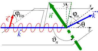
Figure 4: (Colour on-line) Kinematics of ${}^{3}\text{He}$ Compton scattering.

The cross section for Compton scattering of a polarised photon beam with density matrix $\rho^{(\gamma)}$ from a polarised target of spin $S$ with density matrix $\rho^{(S)}$, without detection of the final state polarisations, is found from the Compton tensor $T$ of eq. (2.2) via

$$\frac{\mathrm{d}\sigma}{\mathrm{d}\Omega}=\Phi^{2}\;\mathrm{tr}[T\rho^{(S)}\rho^{(\gamma)}T^{\dagger}]\;\;,$$ (3.2)

where the trace is taken over the polarisation states and $\Phi$ is the frame-dependent flux factor. In the lab frame [40, sect. 2.3]:

$$\Phi_{\mathrm{lab}}=\frac{\omega_{\mathrm{lab}}^{\prime}}{4\pi\omega_{\mathrm{lab}}}\;\;.$$ (3.3)

Two popular bases exist for each density matrix. In the helicity basis, the photon polarisation is described by

$$\left(\rho^{(\gamma)}\right)_{\lambda^{\prime}\lambda}:=\langle\lambda^{\prime}|\rho^{(\gamma)}|\lambda\rangle=\frac{1}{2}\left[\delta_{\lambda^{\prime}\lambda}\left(1+\lambda\;P^{(\gamma)}_{\text{circ}}\right)-\delta_{\lambda^{\prime},-\lambda}\;P^{(\gamma)}_{\text{lin}}\;\mathrm{e}^{+2\lambda\mathrm{i}\varphi_{\text{lin}}}\right]\;\;.$$ (3.4)

Here, positive/negative helicities $\lambda,\lambda^{\prime}=\pm 1$ are defined by $\vec{e}_{\pm}=-\mathrm{i}(\vec{e}_{y}\mp\mathrm{i}\vec{e}_{x})/\sqrt{2}$. $P^{(\gamma)}_{\text{circ}}\in[-1;1]$ is the degree of right-circular polarisation, i.e. the difference between right- and left-circular polarisation, with $P^{(\gamma)}_{\text{circ}}=+1/-1$ describing a fully right-/left-circularly polarised photon. The degree of linear polarisation is $P^{(\gamma)}_{\text{lin}}\in[0;1]$.

In the Cartesian basis, the Stokes parameters $\xi_{i}$ parametrise the $x$ and $y$ components of the density matrix of the incident photon. With $i,j\in\{x;y\}$:

$$\left(\rho^{(\gamma)}\right)_{ij}=\frac{1}{2}\begin{pmatrix}1+\xi_{3}&\xi_{1}-\mathrm{i}\xi_{2}\\ \xi_{1}+\mathrm{i}\xi_{2}&1-\xi_{3}\end{pmatrix}_{ij}\;\;.$$ (3.5)

The degree of right-circular polarisation is then $P^{(\gamma)}_{\text{circ}}=\xi_{2}$, and that of linear polarisation is $P^{(\gamma)}_{\text{lin}}=\sqrt{\xi_{1}^{2}+\xi_{3}^{2}}$, with angle $\cos[2\varphi_{\text{lin}}]=\xi_{3}/\sqrt{\xi_{1}^{2}+\xi_{3}^{2}}$ and $\sin[2\varphi_{\text{lin}}]=\xi_{1}/\sqrt{\xi_{1}^{2}+\xi_{3}^{2}}$, so that $\xi_{i}\in[-1;1]$. The combination $\xi_{3}=\pm 1$, $\xi_{1}=0$ describes a beam which is linearly polarised in/perpendicular to the scattering plane, and $\xi_{1}=\pm 1$ with $\xi_{3}=0$ a beam which is linearly polarised at angle $\varphi_{\text{lin}}=\pm\pi/4$ relative to the scattering plane.

The multipole-decomposition of the density matrix of a polarised spin-$S$ target is [68]:

$$\rho^{(S)}_{m^{\prime}m}:=\langle m^{\prime}|\rho^{(S)}|m\rangle=\frac{(-)^{S-m}}{\sqrt{2S+1}}\sum\limits_{J=0}^{2S}\sqrt{2J+1}\;P^{S}_{J}\sum\limits_{M=-J}^{J}\left(\begin{matrix}S&S&J\\ m&-m^{\prime}&-M\end{matrix}\right)\mathrm{e}^{\mathrm{i}M\varphi_{\vec{n}}}\;d^{J}_{M0}(\vartheta_{\vec{n}})\;\;,$$ (3.6)

where $P^{S}_{0}\equiv 1$ and $P^{\frac{1}{2}}_{1}=P^{(\text{${}^{3}\text{He}$})}$. The conventions for $3j$-symbols and reduced Wigner-$d$ matrices are those of Rose [71], also listed in the Review of Particle Physics [72].

Another variant for spin-$\frac{1}{2}$ particles in the same basis uses Pauli spin matrices $\vec{\sigma}$:

$$\rho^{(\frac{1}{2})}=\frac{1}{2}\bigl{(}1+P^{(\text{${}^{3}\text{He}$})}\;\vec{\sigma}\cdot\vec{n}\bigr{)}\;\;.$$ (3.7)

These variants also lead to different parametrisations of the differential cross section with definite beam and target polarisations (and no detection of the final-state polarisations), after parity invariance has been taken into account. In our analysis, both variants will be used side-by-side:

$$\frac{\mathrm{d}\sigma}{\mathrm{d}\Omega}= \displaystyle\left.\frac{\mathrm{d}\sigma}{\mathrm{d}\Omega}\right|_{\text{unpol}}\;\bigg{[}\;1 +\;\Sigma^{\text{lin}}(\omega,\theta)\;P^{(\gamma)}_{\text{lin}}\;\cos 2\varphi_{\text{lin}}\;+\;T_{11}(\omega,\theta)\;P^{(\text{${}^{3}\text{He}$})}\;d^{1}_{10}(\vartheta_{\vec{n}})\;\sin[\varphi_{\vec{n}}]$$

$$+\sum\limits_{M=0,1}\;T_{1M}^{\text{circ}}(\omega,\theta)\;P^{(\text{${}^{3}\text{He}$})}\;P^{(\gamma)}_{\text{circ}}\;d^{1}_{M0}(\vartheta_{\vec{n}})\;\cos[M\varphi_{\vec{n}}]$$

$$+\sum\limits_{-1\leq M\leq 1}\;T_{1M}^{\text{lin}}(\omega,\theta)\;P^{(\text{${}^{3}\text{He}$})}\;P^{(\gamma)}_{\text{lin}}\;d^{1}_{M0}(\vartheta_{\vec{n}})\;\sin[M\varphi_{\vec{n}}-2\varphi_{\text{lin}}]\bigg{]}$$

$$= \displaystyle\left.\frac{\mathrm{d}\sigma}{\mathrm{d}\Omega}\right|_{\text{unpol}}\;\bigg{[}\;1 +\;\xi_{3}\;\Sigma_{3}(\omega,\theta)\;+\;P^{(\text{${}^{3}\text{He}$})}\,n_{y}\;\Sigma_{y}(\omega,\theta)\,$$

$$+\;P^{(\text{${}^{3}\text{He}$})}\,\xi_{1}\Big{(}n_{x}\;\Sigma_{1x}(\omega,\theta)+n_{z}\;\Sigma_{1z}(\omega,\theta)\Big{)}$$

$$+\;P^{(\text{${}^{3}\text{He}$})}\,\xi_{2}\Big{(}n_{x}\;\Sigma_{2x}(\omega,\theta)+n_{z}\;\Sigma_{2z}(\omega,\theta)\Big{)}\;+\;P^{(\text{${}^{3}\text{He}$})}\,\xi_{3}\;n_{y}\;\Sigma_{3y}(\omega,\theta)\bigg{]}\,.$$

The first one, eq. (3.1), is based on the general multipole decomposition, and was adapted to deuteron Compton scattering in refs. [48, 49]. Its independent observables $T_{JM}^{X}$ carry the target multipolarity $(J,M)$ as subscript and the beam polarisation $X\in\{\mbox{none, circ, lin}\}$ as superscript, and naturally extend to arbitrary-spin targets.

The second one, eq. (3.1), by Babusci et al. [70], uses a Cartesian basis and the components $n_{i}$ of the polarisation vector $\vec{n}$. It uses the indices of the Stokes parameter $\xi_{i}$ and the target polarisation direction $n_{\alpha}$ as the labels of the asymmetries $\Sigma_{i\alpha}$. This form is more convenient to translate rate-difference experiments since typically only one of the parameters $\xi_{i}$ is nonzero.

In either case, the cross section for Compton processes on spin-$\frac{1}{2}$ targets without detecting final-state polarisations is fully parametrised by $8$ linearly independent functions listed below. Here, $\mathrm{d}\sigma$ is shorthand for ${\mathrm{d}\sigma}/{\mathrm{d}\Omega}$; superscripts refer to photon polarisations (“$\parallel$” for polarisation in the scattering plane, “$\perp$” for perpendicular to it); subscripts to target polarisations; and the absence of either means unpolarised. The observables are:

• $1$ differential cross section $\displaystyle\left.\frac{\mathrm{d}\sigma}{\mathrm{d}\Omega}\right|_{\text{unpol}}$ of unpolarised photons on an unpolarised target.

• $1$ beam asymmetry of a linearly polarised beam on an unpolarised target:

  $$\Sigma^{\text{lin}}=\Sigma_{3}=\frac{\mathrm{d}\sigma^{||}-\mathrm{d}\sigma^{\perp}}{\mathrm{d}\sigma^{||}+\mathrm{d}\sigma^{\perp}}\,.$$ (3.10)

• $1$ vector target asymmetry for a target polarised out of the scattering plane along the $\pm y$ direction and an unpolarised beam:

  $$T_{11}=-\sqrt{2}\;\Sigma_{y}=-\sqrt{2}\;\frac{\mathrm{d}\sigma_{y}-\mathrm{d}\sigma_{-y}}{\mathrm{d}\sigma_{y}+\mathrm{d}\sigma_{-y}}\;\;.$$ (3.11)

• $2$ double asymmetries of right-/left-circularly-polarised photons on a target polarised along the $\pm x$ or $\pm z$ directions:

  $$T^{\text{circ}}_{11}=-\sqrt{2}\;\Sigma_{2x}=-\sqrt{2}\;\frac{\mathrm{d}\sigma^{R}_{x}-\mathrm{d}\sigma^{L}_{x}}{\mathrm{d}\sigma^{R}_{x}+\mathrm{d}\sigma^{L}_{x}}\;\;,\;\;T^{\text{circ}}_{10}=\Sigma_{2z}=\frac{\mathrm{d}\sigma^{R}_{z}-\mathrm{d}\sigma^{L}_{z}}{\mathrm{d}\sigma^{R}_{z}+\mathrm{d}\sigma^{L}_{z}}\;\;.$$ (3.12)

• $3$ double asymmetries of linearly-polarised photons on a vector-polarised target:

  $$\begin{split}T^{\text{lin}}_{1\pm 1}=&(\pm\Sigma_{1x}-\Sigma_{3y})/\sqrt{2}\\ &\mbox{ with }\Sigma_{1x}=\frac{\mathrm{d}\sigma^{\pi/4}_{x}-\mathrm{d}\sigma^{-\pi/4}_{x}}{\mathrm{d}\sigma^{\pi/4}_{x}+\mathrm{d}\sigma^{-\pi/4}_{x}}\;\;,\;\;\Sigma_{3y}=\frac{(\mathrm{d}\sigma^{||}_{y}-\mathrm{d}\sigma^{\perp}_{y})-(\mathrm{d}\sigma^{||}_{-y}-\mathrm{d}\sigma^{\perp}_{-y})}{\mathrm{d}\sigma^{||}_{y}+\mathrm{d}\sigma^{\perp}_{y}+\mathrm{d}\sigma^{||}_{-y}+\mathrm{d}\sigma^{\perp}_{-y}}\;\;,\\ T^{\text{lin}}_{10}=&-\Sigma_{1z}=-\frac{\mathrm{d}\sigma^{\pi/4}_{z}-\mathrm{d}\sigma^{-\pi/4}_{z}}{\mathrm{d}\sigma^{\pi/4}_{z}+\mathrm{d}\sigma^{-\pi/4}_{z}}\;\;.\end{split}$$ (3.13)

The decompositions of eqs. (3.1) and (3.1) hold in any frame, but the functions are frame-dependent.

The differences of the rates, $\Delta_{\alpha}$, for the different orientations associated with each asymmetry are important to facilitate run-time estimates. These are the numerators in eqs. (3.10) to (3.13) and can most conveniently be expressed in the Babusci basis:

$$\Delta_{\alpha}=g\;\Sigma_{\alpha}\;\left.\frac{\mathrm{d}\sigma}{\mathrm{d}\Omega}\right|_{\text{unpol}}\;\;,$$ (3.14)

with $g=4$ for $\Delta_{3y}$ and $g=2$ for all other asymmetries [44].

Finally, we provide the translations to the notations used by Hildebrandt et al. [26, 73] and Shukla et al. [1, 2, 3]. The asymmetries are

$$\begin{split}\Sigma_{2x}&=-\frac{T^{\text{circ}}_{11}}{\sqrt{2}}=\Sigma_{x}^{\text{\cite[cite]{[\@@bibref{Number}{Hildebrandt:2005ix, Hildebrandt:2003md,ShuklaPhD, Choudhury:2007bh,Shukla:2008zc}{}{}]}}}\;\;,\\ \Sigma_{2z}&=T^{\text{circ}}_{10}=\Sigma_{z}^{\text{\cite[cite]{[\@@bibref{Number}{Hildebrandt:2005ix, Hildebrandt:2003md,ShuklaPhD, Choudhury:2007bh,Shukla:2008zc}{}{}]}}}\;\;,\end{split}$$ (3.15)

and the corresponding rates are

$$\begin{split}\Delta_{2x}=2\Sigma_{2x}\left.\frac{\mathrm{d}\sigma}{\mathrm{d}\Omega}\right|_{\text{unpol}}&=-\sqrt{2}\;T^{\text{circ}}_{11}\left.\frac{\mathrm{d}\sigma}{\mathrm{d}\Omega}\right|_{\text{unpol}}=2\;\mathcal{D}_{x}^{\text{\cite[cite]{[\@@bibref{Number}{Hildebrandt:2005ix, Hildebrandt:2003md}{}{}]}}}=\Delta_{x}^{\text{\cite[cite]{[\@@bibref{Number}{ShuklaPhD, Choudhury:2007bh,Shukla:2008zc}{}{}]}}}\;\;,\\ \Delta_{2z}=2\Sigma_{2z}\left.\frac{\mathrm{d}\sigma}{\mathrm{d}\Omega}\right|_{\text{unpol}}&=2T^{\text{circ}}_{10}\left.\frac{\mathrm{d}\sigma}{\mathrm{d}\Omega}\right|_{\text{unpol}}=2\;\mathcal{D}_{z}^{\text{\cite[cite]{[\@@bibref{Number}{Hildebrandt:2005ix, Hildebrandt:2003md}{}{}]}}}=\Delta_{z}^{\text{\cite[cite]{[\@@bibref{Number}{ShuklaPhD, Choudhury:2007bh,Shukla:2008zc}{}{}]}}}\;\;.\end{split}$$ (3.16)

3.2 Translating Amplitudes into Observables

The Compton matrix elements of sect. 2.4.1 are provided in the basis of spin projections and photon helicities (dependencies on $\omega,\theta$ and other parameters are dropped for brevity in this section). For ease of presentation, we abbreviate the sum over all polarisations of the squared amplitude:

$$|\mathcal{A}|^{2}\equiv\sum\limits_{M_{i},\lambda_{i}}|A_{M_{i}\lambda_{i}}|^{2}\equiv\sum\limits_{M_{f},\lambda_{f};M_{i},\lambda_{i}}|A^{M_{f}\lambda_{f}}_{M_{i}\lambda_{i}}|^{2}\;\;.$$ (3.17)

Note that we also suppress the indices and summations for straightforward final-state-polarisation sums, as indicated in the second half of Eq. (3.17).

By inserting the density matrices of eqs. (3.4) and (3.6) into eq. (3.2), one obtains the cross section in terms of the amplitudes, as a function of the photon polarisations $P^{(\gamma)}_{\text{circ}}$ and $P^{(\gamma)}_{\text{lin}}$ with polarisation angle $\varphi_{\text{lin}}$ and ${}^{3}\text{He}$ polarisation $P^{(\text{${}^{3}\text{He}$})}$ with orientation $(\vartheta_{\vec{n}},\varphi_{\vec{n}})$. The functional dependence of the result on these parameters is easily matched to the parametrisation in eq. (3.1). For the unpolarised part, the result is:

$$\left.\frac{\mathrm{d}\sigma}{\mathrm{d}\Omega}\right|_{\text{unpol}}=\frac{\Phi^{2}}{4}|\mathcal{A}|^{2}\;.$$ (3.18)

The factor $\frac{1}{4}$ is familiar from averaging over initial spins and helicities. The asymmetries

$$\Sigma^{\text{lin}}\;|\mathcal{A}|^{2} =-\sum\limits_{M_{i},\lambda_{i}}A_{M_{i}\lambda_{i}}A^{*}_{M_{i},-\lambda_{i}}\;,$$ (3.19)

$$T_{11}\;|\mathcal{A}|^{2} =2\sqrt{6}\;\mathrm{i}\sum\limits_{M_{i},M_{i}^{\prime},\lambda_{i}}(-)^{\frac{1}{2}-M_{i}}\left(\begin{matrix}\frac{1}{2}&\frac{1}{2}&1\\ M_{i}&-M_{i}^{\prime}&-1\end{matrix}\right)A_{M_{i}^{\prime}\lambda_{i}}A^{*}_{M_{i}\lambda_{i}}\;,$$ (3.20)

$$T_{1M}^{\text{circ}}\;|\mathcal{A}|^{2} =(2-\delta_{M0})\;\sqrt{6}\;\sum\limits_{M_{i},M_{i}^{\prime},\lambda_{i}}(-)^{\frac{1}{2}-M_{i}}\;\lambda_{i}\left(\begin{matrix}\frac{1}{2}&\frac{1}{2}&1\\ M_{i}&-M_{i}^{\prime}&-M\end{matrix}\right)A_{M_{i}^{\prime}\lambda_{i}}A^{*}_{M_{i}\lambda_{i}}\;,$$ (3.21)

$$T_{1M}^{\text{lin}}\;|\mathcal{A}|^{2} =-\sqrt{6}\;\mathrm{i}\sum\limits_{M_{i},M_{i}^{\prime},\lambda_{i}}(-)^{\frac{1}{2}-M_{i}}\;\lambda_{i}^{M+1}\left(\begin{matrix}\frac{1}{2}&\frac{1}{2}&1\\ M_{i}&-M_{i}^{\prime}&-\lambda_{i}M\end{matrix}\right)A_{M_{i}^{\prime}\lambda_{i}}A^{*}_{M_{i},-\lambda_{i}}\;,$$ (3.22)

can be translated into the Babusci basis using eqs. (3.10) to (3.13).

Since the amplitudes are real below the first inelasticity and $M_{i},M_{i}^{\prime}\in\{\pm\frac{1}{2}\}$, the occurrence of the imaginary unit in four of the observables in eqs. (3.19) to (3.22) indicates that they are zero there, i.e. below the first inelasticity,

$$T_{11}\equiv 0\;\;,\;\;T_{1(0,\pm 1)}^{\text{lin}}\equiv 0\;\;.$$ (3.23)

This is equivalent to the statement that $\Sigma_{y}$, $\Sigma_{1x/z}$ and $\Sigma_{3y}$ are zero in this kinematic region. For ${}^{3}\text{He}$, the first strong inelasticity starts with the knock-out reaction $\gamma\,{}^{3}\text{He}\to\gamma pd$. However, in the regime we are concerned with, nuclear dissociation processes are relatively small and our approach does not include them. In contradistinction, the first appreciable strong-interaction inelasticity on the proton starts at the one-pion production threshold. Hence, in what follows, we study the four observables for which our approach yields non-zero results below the pion-production threshold: the differential cross section, $\Sigma^{\text{lin}}=\Sigma_{3}$, $T_{11}^{\text{circ}}=-\sqrt{2}\;\Sigma_{2x}$, and $T_{10}^{\text{circ}}=\Sigma_{2z}$.

4 Results With Explicit Delta

4.1 Central Values and Variations of the Nucleon Polarisabilities

In this section, we present the results of our calculations, including the sensitivity of several of the observables defined in the previous section to neutron scalar and spin polarisabilities.

Unless otherwise stated, we use the $\mathcal{O}(e^{2}\delta^{3})$ amplitude described above, with the ${}^{3}\text{He}$ wave function in $\chi$EFT calculated using the Idaho potential at N³LO and the “b” version of the 3NI provided by A. Nogga [63, 64]. We will, however, show some results with the $\mathcal{O}(e^{2}\delta^{2})$ amplitude in order to exhibit the impact of adding explicit Deltas to the calculation. At both $\mathcal{O}(e^{2}\delta^{2})$ and $\mathcal{O}(e^{2}\delta^{3})$ we set the proton and neutron scalar polarisabilities to the central values of eqs. (1.2) and (1.1), respectively. Differences between the orders are thus guaranteed not to be contaminated by spurious dependencies on the well-established Baldin sum rules. Indeed, the sensitivity of observables to varying polarisabilities is nearly unaffected by the exact choice of their central values. However, for the central values of the spin polarisabilities for both proton and neutron, we use the values that are predicted by $\chi$EFT at the two orders under consideration [40, 21]:

$$\mathcal{O}(e^{2}\delta^{2})\mbox{ (no Delta):} \hskip 5.0pt\gamma_{E1E1}=5\gamma_{M1M1}=-5\gamma_{E1M2}=-5\gamma_{M1E2}=-5.6\;\;,$$ (4.1)

$$\mathcal{O}(e^{2}\delta^{3})\mbox{ (with Delta):} \hskip 5.0pt\gamma_{E1E1}=-5.1\;,\;\gamma_{M1M1}=3.1\;,\;\gamma_{E1M2}=\gamma_{M1E2}=0.9\;\;.$$ (4.2)

Therefore, the amplitudes at these two orders differ by terms at $\mathcal{O}(\omega^{3})$. At the next $\chi$EFT order, $\mathcal{O}(e^{2}\delta^{4})$, proton and neutron spin-polarisability values differ. Results, including theory uncertainties, can be found in ref. [21]. The corrections to the $\mathcal{O}(e^{2}\delta^{3})$ values are less than $2$ canonical units.

As discussed around eq. (1.2), the scalar polarisabilities of the proton are known to much better accuracy than the neutron ones. Furthermore, given the current state of few-body theory, more accurate values of proton polarisabilities will come from proton data than from $\gamma{}^{3}$He scattering. Therefore, for our current study of ${}^{3}\text{He}$, we only consider variations of the six neutron scalar and spin polarisabilities about the baseline values of eqs. (1.1) and (4.2), and explore the pattern of sensitivities to such variations across different observables. As in the study of deuteron asymmetries in refs. [47, 48, 49], we choose a variation of the polarisabilities by $\pm 2$ canonical units. This is roughly at the level of the combined statistical, theoretical and Baldin sum rule induced uncertainties of the scalar polarisabilities of the neutron, and also is about the combined uncertainty of the spin polarisabilities [44]. These changes are implemented by adding the following term,

$$\begin{split}{T}^{\mathrm{var}}(\omega,\,z=\cos\theta_{\mathrm{cm}})=&4\pi\,\omega^{2}\,\bigg{[}[\delta\alpha_{E1}+z\,\delta\beta_{M1}]\,(\vec{\epsilon}^{\,\prime\ast}\cdot\vec{\epsilon})-\delta\beta_{M1}\,(\vec{\epsilon}^{\,\prime\ast}\cdot\hat{k})\,(\vec{\epsilon}\cdot\hat{k}^{\prime})\\ &-\mathrm{i}\,[\delta\gamma_{E1E1}+z\,\delta\gamma_{M1M1}+\delta\gamma_{E1M2}+z\,\delta\gamma_{M1E2}]\,\omega\,\vec{\sigma}\cdot(\vec{\epsilon}^{\,\prime\ast}\times\vec{\epsilon})\\ &+\mathrm{i}\,[\delta\gamma_{M1E2}-\delta\gamma_{M1M1}]\,\omega\,\vec{\sigma}\cdot\left(\hat{k}^{\prime}\times\hat{k}\right)(\vec{\epsilon}^{\,\prime\ast}\cdot\vec{\epsilon})\\ &+\mathrm{i}\,\delta\gamma_{M1M1}\,\omega\,\vec{\sigma}\cdot\left[\left(\vec{\epsilon}^{\,\prime\ast}\times\hat{k}\right)(\vec{\epsilon}\cdot\hat{k}^{\prime})-\left(\vec{\epsilon}\times\hat{k}^{\prime}\right)(\vec{\epsilon}^{\,\prime\ast}\cdot\hat{k})\right]\\ &+\mathrm{i}\,\delta\gamma_{E1M2}\,\omega\,\vec{\sigma}\cdot\left[\left(\vec{\epsilon}^{\,\prime\ast}\times\hat{k}^{\prime}\right)(\vec{\epsilon}\cdot\hat{k}^{\prime})-\left(\vec{\epsilon}\times\hat{k}\right)(\vec{\epsilon}^{\,\prime\ast}\cdot\hat{k})\right]\bigg{]}\;\;,\end{split}$$ (4.3)

to the single-nucleon amplitude in the $\gamma$N cm frame. Note that changing $\alpha_{E1}^{(\mathrm{n})}-\beta_{M1}^{(\mathrm{n})}$ by $+2$ units while keeping $\alpha_{E1}^{(\mathrm{n})}+\beta_{M1}^{(\mathrm{n})}$ fixed translates to a concurrent variation of $\alpha_{E1}^{(\mathrm{n})}$ by $+1$ unit and $\beta_{M1}^{(\mathrm{n})}$ by $-1$ unit. Other variations are quite well determined by linear extrapolation from our results, since quadratic contributions of the polarisability variations $\delta(\alpha_{E1},\beta_{M1},\gamma_{i})$ are suppressed in the squared amplitudes.

The sensitivities could be visualised using the “heat maps” employed for proton observables in ref. [44]. However, there is no data for elastic Compton scattering on ${}^{3}\text{He}$ and theory is currently constrained to a smaller energy range, $50\;\mathrm{MeV}\lesssim\omega_{\mathrm{lab}}\lesssim 120\;\mathrm{MeV}$, where the rates and sensitivities vary much less than they do in the wider energy range of the proton study. For this exploratory study, we therefore decided to concentrate on results at two extreme energies: $\omega_{\mathrm{lab}}\approx 60\;\mathrm{MeV}$, where only effects from varying the scalar polarisabilities are seen, and $\omega_{\mathrm{lab}}\approx 120\;\mathrm{MeV}$, where spin polarisabilities are contributing appreciably as well. More detailed questions about sensitivities and constraints, such as on $\gamma_{0}$ and $\gamma_{\pi}$, are deferred to a future study in which we extend the present formalism above the pion-production threshold and one order further, i.e. to $\mathcal{O}(e^{2}\delta^{4})$ [50].

4.2 Corrections to Previous Presentations

The analytic formulae for Feynman diagrams in refs. [3, 1] are correct. However, the code that calculated observables for Compton scattering from ${}^{3}\text{He}$ contained the following errors in the implementation of the two-nucleon Compton operator that appears at $\mathcal{O}(Q^{3}=e^{2}\delta^{2})$ in the chiral expansion:

1. It failed to include the isospin dependence $(\tau^{(1)}\cdot\tau^{(2)}-\tau^{(1)}_{3}\tau^{(2)}_{3})/2$ of the two-nucleon operator; see ref. [3, eq. (59)]. This factor is $1$ for “deuteron”-like pairs and $-1$ for isospin-$1$ $np$ pairs. ($pp$ and $nn$ pairs do not contribute at this order.)

2. A factor of two was missed when coding the operator that produces transitions between pairs where the two-nucleon spin changes $s_{12}=0\leftrightarrow s_{12}=1$.

3. There was a mistake in the implementation of the $s_{12}=0\leftrightarrow s_{12}=1$ piece of the third diagram in fig. 2.

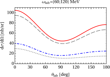
Figure 5: (Colour on-line) The lab-frame ${}^{3}\text{He}$ cross section at $\mathcal{O}(e^{2}\delta^{2})$ [N²LO, no explicit Delta] at $\omega_{\mathrm{lab}}=60\;\mathrm{MeV}$ after (solid red) and before (dashed gray) corrections; and at $\omega_{\mathrm{lab}}=120\;\mathrm{MeV}$ after (dot-dashed blue) and before (dotted gray) corrections. Here, and only here, we use the $\mathcal{O}(e^{2}\delta^{2})$ polarisability values for both protons and neutrons, $\alpha_{E1}^{(\mathrm{p})}=\alpha_{E1}^{(\mathrm{n})}=10\beta_{M1}^{(\mathrm{p})}=10\beta_{M1}^{(\mathrm{n})}=12.5$, in order to be consistent with the choice of refs. [1, 2, 3].

Of these, the first mistake had the largest consequences. The others only affected parts of the matrix element that involve small pieces of the ${}^{3}\text{He}$ wave function. But rectifying the isospin factor increases the prediction for the cross section markedly: by about $10\%$ at $\omega_{\mathrm{lab}}\approx 60\;\mathrm{MeV}$, and by as much as $40\%$ ($80\%$) at forward (backward) angles at $120\;\mathrm{MeV}$. Figure 5 compares the corrected and original lab cross sections at $60$ and $120\;\mathrm{MeV}$ at $\mathcal{O}(e^{2}\delta^{2})$ (without explicit Delta), using the same parameters as the original publications [3, 1]. Corrections for $\Sigma^{\text{lin}}=\Sigma_{3}$ are minimal; $T^{\text{circ}}_{11}=-\sqrt{2}\,\Sigma_{2x}$ and $T^{\text{circ}}_{10}=\Sigma_{2z}$ reduce by less than $5\%$ at $\omega_{\mathrm{lab}}\approx 60\;\mathrm{MeV}$ (rates increase by about $5\%$), and by less than $14\%$ at $\omega_{\mathrm{lab}}\approx 120\;\mathrm{MeV}$ (rates increase by $16\%$).

Previous investigations of deuteron Compton scattering [23, 26, 25, 27, 46, 47, 48, 49] use the same two-nucleon amplitudes, so it is important to stress that these issues only affect the ${}^{3}\text{He}$ calculation, and not that for the deuteron ($s_{12}=1$, $t_{12}=0$).

4.3 Differential Cross Section

We now turn our attention to the $\mathcal{O}(e^{2}\delta^{3})$ results for the elastic cross section. Figure 6 shows that there is a steady decrease of the cross section between $50\;\mathrm{MeV}$ and $120\;\mathrm{MeV}$ for all angles. Meanwhile, the forward-backward difference, which is about 20% at $50\;\mathrm{MeV}$, essentially disappears by $120\;\mathrm{MeV}$.

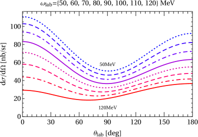
Figure 6: (Colour on-line) The ${}^{3}\text{He}$ cross section at $\mathcal{O}(e^{2}\delta^{3})$, for $\omega_{\mathrm{lab}}$ between $50\;\mathrm{MeV}$ (top-most line) and $120\;\mathrm{MeV}$ (bottom-most line) in $10\;\mathrm{MeV}$ steps.

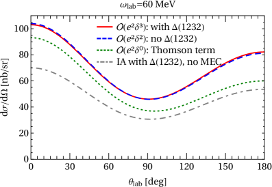
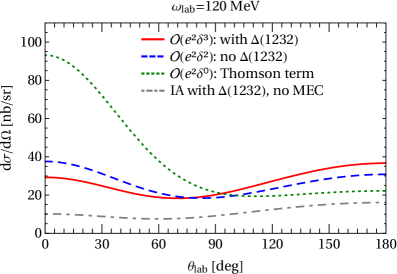
Figure 7: (Colour on-line) The ${}^{3}\text{He}$ cross section at orders $e^{2}\delta^{3}$ (with Delta; red solid), $e^{2}\delta^{2}=Q^{3}$ (blue dashed) and $e^{2}\delta^{0}=Q^{2}$ (single-nucleon-Thomson term only; green dotted) at $\omega_{\mathrm{lab}}=60\;\mathrm{MeV}$ (left) and $120\;\mathrm{MeV}$ (right). We also show an incomplete “Impulse Approximation” calculation that includes $\mathcal{O}(e^{2}\delta^{3})$ single-nucleon (with Delta) amplitudes but not two-body currents (gray dot-dashed). Note that here, and in subsequent order-by-order comparisons, at ${\cal O}(e^{2}\delta^{2})$ and ${\cal O}(e^{2}\delta^{3})$ the scalar polarisabilities are fixed to the same values, eqs. (1.1) and (1.2), but the spin polarisabilities differ; see eqs. (4.1) and (4.2).

Figure 7 shows that the order-by-order convergence is good over the range of applicability. The single-nucleon-Thomson term of fig. 1(a) constitutes LO [$\mathcal{O}(e^{2}\delta^{0})$] and indeed provides the bulk of the cross section. Only for extreme forward scattering at the highest energies, $\omega_{\mathrm{lab}}\gtrsim 110\;\mathrm{MeV}$, does the next nonzero correction, $\mathcal{O}(e^{2}\delta^{2})$, lead to a $60\%$ reduction. The order at which the Delta enters [N³LO, $\mathcal{O}(e^{2}\delta^{3})$] provides a parametrically small correction to N²LO [$\mathcal{O}(e^{2}\delta^{2})$] when the same values for the scalar polarisabilities are chosen. At low energies, the variants with [$\mathcal{O}(e^{2}\delta^{3})$] and without [$\mathcal{O}(e^{2}\delta^{2})$] explicit Delta are near-indistinguishable. The difference is about $25\%$ at the highest energy considered here, $\omega_{\mathrm{lab}}=120\;\mathrm{MeV}$. Note, though, that the angular dependence is substantially changed once the Delta is included: backward-angle scattering increases and forward-angle scattering decreases.

Such a strong signal from the $\Delta(1232)$ below the pion production threshold might at first be surprising. However, even though the effect of the Delta on the scalar polarisabilities is hidden by using their fitted values in both orders, eqs. (4.1) and (4.2) show that the value of $\gamma_{M1M1}$ differs at $\mathcal{O}(e^{2}\delta^{2})$ and $\mathcal{O}(e^{2}\delta^{3})$, i.e., without and with the Delta. More important, though, are the sizeable dispersive corrections to $\beta_{M1}$ induced by the $\Delta$. These cannot be absorbed into the static value of $\beta_{M1}$. At $\omega=120\;\mathrm{MeV}$, their impact on observables can be as large as that of $\beta_{M1}$ itself; see also the discussion and plots of “dynamic polarisabilities” in refs. [40, 44].

Figure 7 also includes the results of an “impulse approximation” (IA) calculation in which the two-body-current contribution is artificially set to zero. This calculation is not consistent with the $\chi$EFT power counting, since this effect is $\mathcal{O}(e^{2}\delta^{2})$. Comparing the IA result to the $\mathcal{O}(e^{2}\delta^{0})$ (i.e. single-nucleon-Thomson only) result shows that structure effects in the single-nucleon Compton amplitudes lead to significant suppression of the cross section, just as for proton Compton scattering (particularly obvious in fig. 3 of ref. [74]). However, in the full $\mathcal{O}(e^{2}\delta^{2})$ result at $60\;\mathrm{MeV}$, this suppression is more than compensated by two-body currents that increase the ${}^{3}\text{He}$ Compton cross section by roughly a factor of two over the IA result. Two-body currents play an even larger fractional role at higher energies. This confirms, yet again, the findings for Compton scattering on ${}^{3}\text{He}$ in refs. [2, 3, 1], and on the deuteron in ref. [23], that two-body currents must be included in any realistic description of few-nucleon Compton scattering.

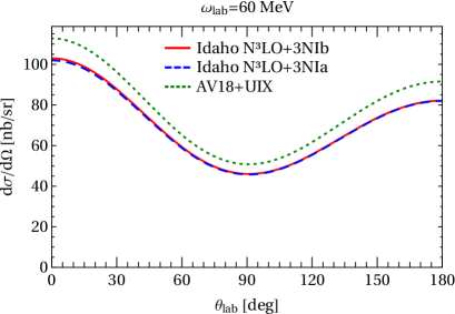
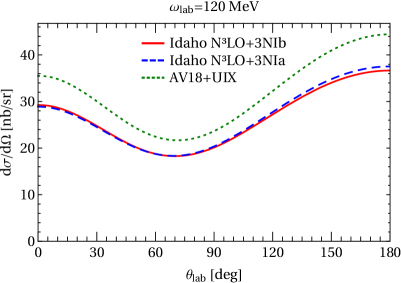
Figure 8: (Colour on-line) The ${}^{3}\text{He}$ cross section for different ${}^{3}\text{He}$ wave functions in the lab frame at $\omega_{\mathrm{lab}}=60\;\mathrm{MeV}$ (left) and $120\;\mathrm{MeV}$ (right): $\chi$EFT’s Idaho variant at N³LO with 3NI “b” (red solid); $\chi$EFT’s Idaho variant at N³LO with 3NI “a” (blue dashed); AV18 with Urbana-IX 3NI (green dotted). Notice the difference of scales.

In fig. 8, we compare the results for the three different ${}^{3}\text{He}$ wave functions discussed in sect. 2.4.2: $\chi$EFT (Idaho formulation) at N³LO with 3NI “b” or “a”, and AV18 with the Urbana-IX 3NI. The wave functions of the two $\chi$EFT variants yield near-identical results. As anticipated, there is a larger difference between these two and AV18 with the Urbana-IX 3NI: this wave function leads to cross sections which are about 10% larger at lower energies, and $\approx 20\%$ larger at $\omega_{\mathrm{lab}}=120\;\mathrm{MeV}$. The effect of these discrepancies is mitigated by the fact that the relative difference in the predicted cross section in fig. 8 is largely angle independent, whereas we see in fig. 9 that the sensitivities to the scalar polarisabilities have a rather strong angular dependence.

The difference induced by varying the scalar polarisabilities of the neutron by $\pm 2$ units at $\omega_{\mathrm{lab}}=60\;\mathrm{MeV}$ hardly exceeds the thickness of the line. At $\omega_{\mathrm{lab}}=120\;\mathrm{MeV}$, such a variation results in cross section variations of $\lesssim\pm 8\%$ or $\pm 1$nb/sr. Equivalent polarisability variations in the deuteron case lead to changes in the cross section that are smaller in absolute terms, but represent a larger fraction of the (much) smaller cross section for that process. At both energies, varying the spin polarisabilities by up to $\pm 100\%$ of their baseline values (or at least $\pm 2$ canonical units) produces variations which are at most as large as the line thickness.

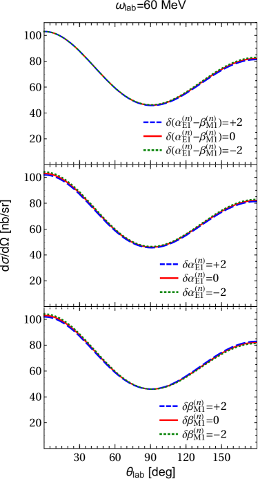
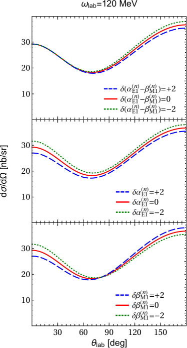
Figure 9: (Colour on-line) Sensitivity of the cross section to varying the scalar polarisabilities of the neutron $\alpha_{E1}^{(\mathrm{n})}-\beta_{M1}^{(\mathrm{n})}$ (top), $\alpha_{E1}^{(\mathrm{n})}$ (middle) and $\beta_{M1}^{(\mathrm{n})}$ (bottom) about their central values ( ) of eq. (1.1) by $+2$ (       ) and $-2$ ($\cdot$ $\cdot$ $\cdot$ $\cdot$ $\cdot$ $\cdot$ ) units, at $\omega_{\mathrm{lab}}=60\;\mathrm{MeV}$ (left) and $120\;\mathrm{MeV}$ (right). Even at $\omega_{\mathrm{lab}}=120\;\mathrm{MeV}$, changes in the spin polarisabilities produces variations which are at most as large as the thickness of the line. Notice the difference of the scales.

4.4 Beam Asymmetry

We start our discussion of the observables for polarised beams and/or targets with the beam asymmetry $\Sigma^{\mathrm{lin}}=\Sigma_{3}$; see eq. (3.10). As shown in the top row of fig. 10, its magnitude and shape do not change significantly between $\omega_{\mathrm{lab}}=50\;\mathrm{MeV}$ and $120\;\mathrm{MeV}$. The rate difference $\Delta_{3}$ declines steadily: at $\omega_{\mathrm{lab}}=120\;\mathrm{MeV}$ it is one third of its value at $50\;\mathrm{MeV}$. This is also by far the largest asymmetry, near-saturating the extreme value of $-1$ around $\theta_{\mathrm{lab}}=90^{\circ}$.

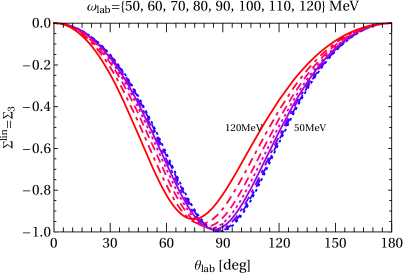
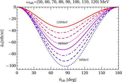
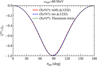
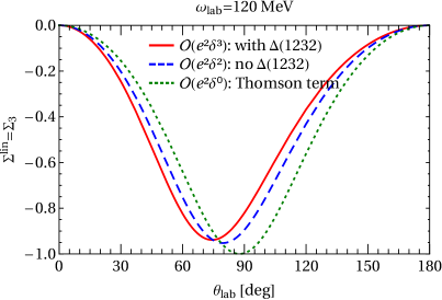
Figure 10: (Colour on-line) The beam asymmetry $\Sigma^{\mathrm{lin}}=\Sigma_{3}$ in the lab frame. Top: Energies between $\omega_{\mathrm{lab}}=50\;\mathrm{MeV}$ and $120\;\mathrm{MeV}$ in $10\;\mathrm{MeV}$ steps, for the asymmetry (left) and the corresponding rate difference (right). Bottom: order-by-order convergence at $\omega_{\mathrm{lab}}=60\;\mathrm{MeV}$ (left) and $120\;\mathrm{MeV}$ (right), with notation as in fig. 7.

As the second row of fig. 10 shows, these features follow from the fact that the beam asymmetry is dominated by the single-nucleon Thomson term. This is also why it is the only asymmetry that is nonzero for $\omega=0$: Compton scattering on a charged point-like particle leads to the $(\cos^{2}\theta-1)/(\cos^{2}\theta+1)$ shape at zero energy which is well-known from Classical Electrodynamics [75]. Even at the highest energies considered here, the nucleons’ magnetic moments and structure change the asymmetry by less than $10\%$, indicating that this observable converges rapidly in $\chi$EFT. All this makes it unsurprising that the wave function dependence is very small, and so we do not display it here.

Given the persistence of this point-like behaviour, it should come as no surprise that there is very little sensitivity to polarisabilities. In fig. 11 we show what variation of $\alpha_{E1}^{(\mathrm{n})}-\beta_{M1}^{(\mathrm{n})}$ and $\beta_{M1}^{(\mathrm{n})}$ do to $\Sigma^{\mathrm{lin}}=\Sigma_{3}$. Even where the effect is largest, at $120\;\mathrm{MeV}$, it is still slight. Varying the electric scalar polarisabilities or the spin ones impacts the beam symmetry even in extreme cases by hardly more than the thickness of the lines (cf. ref. [46] for analytic arguments for this behaviour in the deuteron case).

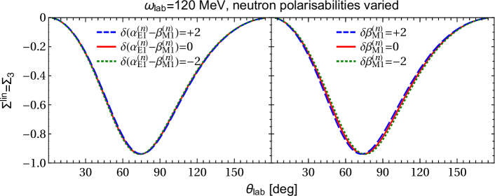
Figure 11: (Colour on-line) Sensitivity of $\Sigma^{\mathrm{lin}}=\Sigma_{3}$ to varying the scalar polarisabilities of the neutron $\alpha_{E1}^{(\mathrm{n})}-\beta_{M1}^{(\mathrm{n})}$ (left) and $\beta_{M1}^{(\mathrm{n})}$ (right) about their central values ( ) of eqs. (1.1) by $+2$ (       ) and $-2$ ($\cdot$ $\cdot$ $\cdot$ $\cdot$ $\cdot$ $\cdot$ ) units, at $\omega_{\mathrm{lab}}=120\;\mathrm{MeV}$. The effect of spin-polarisability variations is considerably exceeded by the thickness of the lines.

4.5 Circularly Polarised Beam on Transversely Polarised Target

Figure 12 shows results for the double asymmetry $T_{11}^{\mathrm{circ}}=-\sqrt{2}\;\Sigma_{2x}$ of eq. (3.12), which is formed by considering scattering of a circularly polarised beam on a target polarised in the $+x$ vs. $-x$ direction. Like the beam asymmetry, it is zero at $\theta=0^{\circ},180^{\circ}$; unlike $\Sigma^{\text{lin}}$, this asymmetry vanishes as $\omega_{\mathrm{lab}}\rightarrow 0$, and is consequently quite small (maximum value of $0.1$) at $\omega_{\mathrm{lab}}=50\;\mathrm{MeV}$. It grows faster than linearly with $\omega_{\mathrm{lab}}$, with a maximum value at $120\;\mathrm{MeV}$ of $0.5$. The corresponding rate difference $\Delta_{2x}$ increases more slowly, by about $50\%$ between $50\;\mathrm{MeV}$ and $120\;\mathrm{MeV}$, because the cross section decreases with energy. Nevertheless, the figure-of-merit for the asymmetry measurement is larger at higher energies—and so, of course, is the sensitivity of the asymmetry to spin polarisabilities. Even though the asymmetry is zero at LO [$\mathcal{O}(e^{2}\delta^{0})$, single-nucleon Thomson term], the $\chi$EFT result converges well (see third panel of fig. 12). The correction from including the Delta at $\mathcal{O}(e^{2}\delta^{3})$ is $25\%$ even at $\omega_{\mathrm{lab}}=120\;\mathrm{MeV}$, and less than $5\%$ at $\omega_{\mathrm{lab}}=60\;\mathrm{MeV}$. The wave function dependence—displayed at $120\;\mathrm{MeV}$ in the fourth panel of fig. 12—is about $\pm 10\%$ and essentially energy-independent. We observe that—as for the differential cross section and $\Sigma^{\mathrm{lin}}=\Sigma_{3}$—all wave functions predict the same shape.

Figure 13 shows the effect of varying the polarisabilities. The upper two panels of fig. 13 show that, even at $\omega_{\mathrm{lab}}=120\;\mathrm{MeV}$, there is little sensitivity to the scalar polarisabilities, especially if the Baldin sum rule constraint on $\alpha_{E1}^{(\mathrm{n})}+\beta_{M1}^{(\mathrm{n})}$ is imposed.

The largest sensitivity is to the spin polarisability $\gamma_{M1M1}^{(\mathrm{n})}$. Changing it by $\pm 2$ units affects $T_{11}^{\mathrm{circ}}$ by about $\pm 8\%$ of its peak value at $\theta_{\mathrm{lab}}\approx 90^{\circ}$ and $\omega_{\mathrm{lab}}=120\;\mathrm{MeV}$. Changes in the other spin polarisabilities produce noticeably smaller effects. Varying $\gamma_{E1M2}^{(\mathrm{n})}$ alters $T_{11}^{\mathrm{circ}}$ more at $\theta_{\mathrm{lab}}<90^{\circ}$; varying $\gamma_{E1E1}^{(\mathrm{n})}$ affects it at $\theta_{\mathrm{lab}}>90^{\circ}$; the sensitivity to $\gamma_{M1E2}^{(\mathrm{n})}$ vanishes at $90^{\circ}$. Therefore, a measurement around $\theta_{\mathrm{lab}}\approx 90^{\circ}$ provides a good opportunity to extract $\gamma_{M1M1}^{(\mathrm{n})}$ with little contamination from the other polarisabilities.

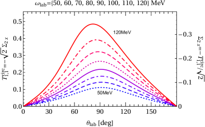
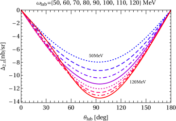
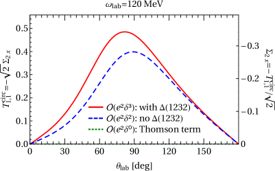
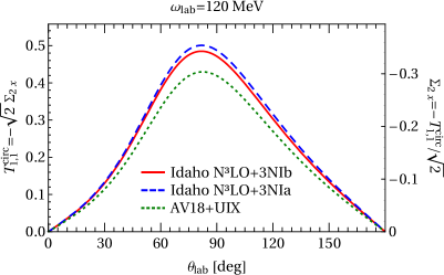
Figure 12: (Colour on-line) The double asymmetry $T_{11}^{\mathrm{circ}}=-\sqrt{2}\;\Sigma_{2x}$ in the lab frame. Top: Energies between $\omega_{\mathrm{lab}}=50\;\mathrm{MeV}$ and $120\;\mathrm{MeV}$ in $10\;\mathrm{MeV}$ steps, for the asymmetry (left) and rate difference (right). Bottom left: order-by-order convergence at $\omega_{\mathrm{lab}}=120\;\mathrm{MeV}$, with notation as in fig. 7; the LO result is identically zero. Bottom right: wave function dependence at $\omega_{\mathrm{lab}}=120\;\mathrm{MeV}$, with notation as in fig. 8.

For this observable, the multipole basis for the spin polarisabilities exhibits a predominant sensitivity to a single spin polarisability. Figure 15 of Shukla et al. [3] shows noticeable effects when two of the spin polarisabilities in the “Ragusa” basis, namely $\gamma_{4}=\gamma_{M1M1}$ and $\gamma_{1}=-\gamma_{E1E1}-\gamma_{E1M2}$, were varied by $\pm 100\%$. The substantial shifts on varying $\gamma_{1}$ largely reflected the fact that it is the largest to start with at ${\cal O}(e^{2}\delta^{2})$. In contrast, our work considers variations of $\pm 2$ units. Allowing for this, the results of ref. [3] and the current work are in fact consistent and serve to show that the multipole basis is more convenient for this observable. In that spirit, we also briefly comment—although we do not show explicit results—that when the forward- and backward-combinations $\gamma_{0/\pi}$ of the spin-polarisabilities are used as constraints, the signal is still strong, as is the one for the combination $\gamma_{M1M1}^{(\mathrm{n})}-\gamma_{M1E2}^{(\mathrm{n})}$ which also appears in the alternative multipole basis introduced in ref. [44].

Finally, we see that an explicit Delta increases both the magnitude of the asymmetry (fig. 12) and its sensitivity to the polarisabilities, compared to the $\mathcal{O}(e^{2}\delta^{2})$-result.

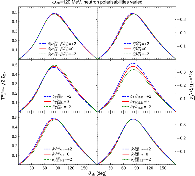
Figure 13: (Colour on-line) Sensitivity of $T_{11}^{\mathrm{circ}}=-\sqrt{2}\;\Sigma_{2x}$ to variations of the neutron polarisabilities $\alpha_{E1}^{(\mathrm{n})}-\beta_{M1}^{(\mathrm{n})}$ (top left), $\alpha_{E1}^{(\mathrm{n})}$ (top right), $\gamma_{E1E1}^{(\mathrm{n})}$ (centre left), $\gamma_{M1M1}^{(\mathrm{n})}$ (centre right), $\gamma_{E1M2}^{(\mathrm{n})}$ (bottom left), and $\gamma_{M1E2}^{(\mathrm{n})}$ (bottom right), about their central values by $\pm 2$ units, at $\omega_{\mathrm{lab}}=120\;\mathrm{MeV}$. Notation as in fig. 11.

4.6 Circularly Polarised Beam on Longitudinally Polarised Target

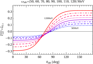
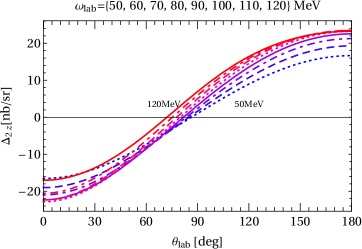
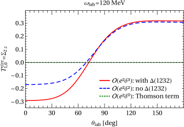
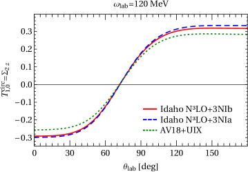
Figure 14: (Colour on-line) The double asymmetry $T_{10}^{\mathrm{circ}}=\Sigma_{2z}$ in the lab frame. Top: Energies between $\omega_{\mathrm{lab}}=50\;\mathrm{MeV}$ and $120\;\mathrm{MeV}$ in $10\;\mathrm{MeV}$ steps, for the asymmetry (left) and rate difference (right). Bottom left: order-by-order convergence at $\omega_{\mathrm{lab}}=120\;\mathrm{MeV}$, with notation as in fig. 7; the LO result is identically zero. Bottom right: wave function dependence at $\omega_{\mathrm{lab}}=120\;\mathrm{MeV}$, with notation as in fig. 8.

Finally, we turn to the double asymmetry $T_{10}^{\mathrm{circ}}=\Sigma_{2z}$ of a circularly polarised beam on a target which is polarised parallel vs. antiparallel to the beam direction; see eq. (3.12). Our predictions are shown in fig. 14. The asymmetry is again zero at LO [$\mathcal{O}(e^{2}\delta^{0})$, single-nucleon Thomson term], and is about the same size as $T_{11}^{\mathrm{circ}}$. It is also zero for $\omega=0$, but nonzero at $\theta=0^{\circ},180^{\circ}$. The upper two panels show that it increases by a factor of about $4$ between $\omega_{\mathrm{lab}}=50\;\mathrm{MeV}$ and $120\;\mathrm{MeV}$. However, the concomitant decrease of the cross section with energy now produces a rate difference that is essentially constant with photon energy. At $\omega_{\mathrm{lab}}=50\;\mathrm{MeV}$ the change from $\mathcal{O}(e^{2}\delta^{2})$ to $\mathcal{O}(e^{2}\delta^{3})$ is at most 5%; order-by-order results at $\omega_{\mathrm{lab}}=120\;\mathrm{MeV}$ are displayed in the third panel of fig. 14. The $\chi$EFT result converges well, showing a significant change from the $\mathcal{O}(e^{2}\delta^{2})$ result only at high energies and forward angles. The wave function dependence is small at all energies and angles; the fourth panel of fig. 14 is quite representative.

Figure 15 shows that variation of the scalar polarisabilities around the baseline values of eq. (1.1) has even less impact on $T_{10}^{\mathrm{circ}}$ than on $T_{11}^{\mathrm{circ}}$.

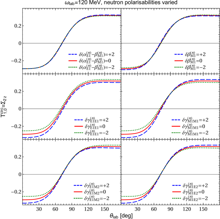
Figure 15: (Colour on-line) Sensitivity of $T_{10}^{\mathrm{circ}}=\Sigma_{2z}$ to varying the scalar and spin polarisabilities of the neutron about their central values by $\pm 2$ units, at $\omega_{\mathrm{lab}}=120\;\mathrm{MeV}$. Notation and panels as in fig. 13.

To maximise sensitivity to the spin polarisabilities, we again show results at $\omega_{\mathrm{lab}}=120\;\mathrm{MeV}$. This time there is no one multipole-basis spin polarisability that shows a unique signal: $\gamma_{E1E1}^{(\mathrm{n})}$ and $\gamma_{E1M2}^{(\mathrm{n})}$ are essentially degenerate with one another, as are $\gamma_{M1M1}^{(\mathrm{n})}$ and $\gamma_{M1E2}^{(\mathrm{n})}$. We briefly comment without showing figures that the results in the alternative multipole basis of the spin polarisabilities proposed in ref. [44] indeed show cleaner signals for the combinations $\gamma_{E1E1}^{(\mathrm{n})}-\gamma_{E1M2}^{(\mathrm{n})}$ and $\gamma_{M1M1}^{(\mathrm{n})}-\gamma_{M1E2}^{(\mathrm{n})}$. $\gamma_{E1E1}^{(\mathrm{n})}$ could possibly be extracted by measuring the point where $T_{10}^{\mathrm{circ}}$ is zero, as the effect of other spin polarisabilities is markedly smaller there. For $\omega_{\mathrm{lab}}=120\;\mathrm{MeV}$, the zero-crossing at $\theta_{\mathrm{lab}}\approx 84^{\circ}$ varies by $\pm 2.5^{\circ}$ for $\delta\gamma_{E1E1}^{(\mathrm{n})}=\pm 2$.

5 Summary, Observations and Outlook

We presented $\chi$EFT predictions with a dynamical Delta degree of freedom at N³LO [$\mathcal{O}(e^{2}\delta^{3})$] for Compton scattering from ${}^{3}\text{He}$ for photon lab energies between $50$ and $120\;\mathrm{MeV}$. We showed results for the differential cross section, for the beam asymmetry $\Sigma^{\mathrm{lin}}=\Sigma_{3}$, and for the two double asymmetries with circularly polarised photons and transversely or longitudinally polarised targets, $T_{11}^{\mathrm{circ}}=-\sqrt{2}\,\Sigma_{2x}$ and $T_{10}^{\mathrm{circ}}=\Sigma_{2z}$. These are the only observables that are non-zero below pion-production threshold in our formulation. We also corrected previous results in refs. [2, 3, 1] for these observables at N²LO [$\mathcal{O}(e^{2}\delta^{2}=Q^{3})$, without dynamical Delta] (see concurrent erratum [4]). As expected, the dynamical effects of the Delta do not enter at low energies, but they are visible in all observables at the upper end of the energy range. In particular, they markedly reduce the forward-backward asymmetry of the cross section and increase the magnitude of the double asymmetries and their sensitivity to spin polarisabilities, echoing similar findings for the deuteron [26, 27, 40, 48, 49].

We showed that the convergence of the chiral expansion in this energy range is quite good. The dependence of the results on the choice of ${}^{3}\text{He}$ wave function is not large, either, and can usually be distinguished from the effects of neutron polarisabilities by its different angular dependence. We found that $\alpha_{E1}^{(\mathrm{n})}-\beta_{M1}^{(\mathrm{n})}$ could be extracted from the cross section, and $T_{11}^{\mathrm{circ}}=-\sqrt{2}\;\Sigma_{2x}$ has a non-degenerate sensitivity to $\gamma_{M1M1}^{(\mathrm{n})}$ around $90^{\circ}$. $T_{10}^{\mathrm{circ}}=\Sigma_{2z}$ is sensitive to $\gamma_{E1E1}^{(\mathrm{n})}$ and $\gamma_{E1M2}^{(\mathrm{n})}$. $\Sigma^{\mathrm{lin}}=\Sigma_{3}$ is a useful cross-check on the accuracy of the $\chi$EFT amplitudes, but is dominated by the single-nucleon Thomson term to surprisingly high energies, and so measurements of this may not be especially useful for polarisability determinations.

Ultimately, the most accurate values of polarisabilities will be inferred from a data set that includes all four observables. For the spin polarisabilities, the upper end of our energy range will be crucial, as the sensitivities at $\omega_{\mathrm{lab}}\lesssim 100\;\mathrm{MeV}$ are so small that discriminating between different spin-polarisability values would be very challenging.

As in ref. [44], we argue that our results can be considered quite robust, i.e. that varying the single-nucleon amplitudes of complementary theoretical approaches like dispersion relations will lead to sensitivities which are hardly discernible from ours. We did not quantify residual theoretical uncertainties in detail, as this presentation is meant to provide an exploratory study of magnitudes and sensitivities of observables to the nucleon polarisabilities. Once data are available, a polarisability extraction will of course need to address residual theoretical uncertainties with more diligence, as was already done for the proton and deuteron in refs. [40, 41, 31, 32, 21].

Our exploration of different observables is therefore sufficient to assess experimental feasibilities, and we see it as part of an ongoing dialogue on the best kinematics and observables for future experiments to obtain information on neutron polarisabilities [5, 6, 8, 7]. To facilitate that dialogue, our results are available as an interactive Mathematica notebook from hgrie@gwu.edu, where cross sections, rates and asymmetries are explored when the scalar and spin polarisabilities are varied, including variations constrained by sum rules.

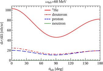
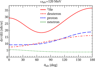
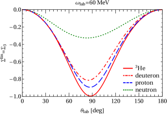
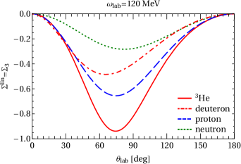
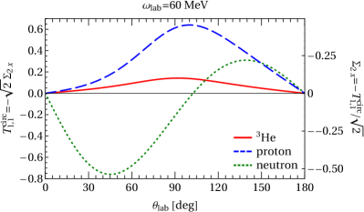
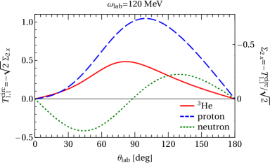
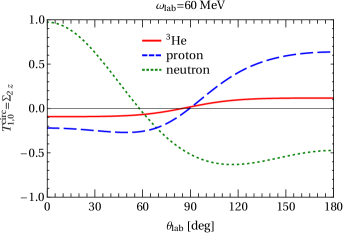
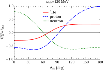
Figure 16: (Colour on-line) Observables at $\mathcal{O}(e^{2}\delta^{3})$ (i.e. with Delta) for $\omega_{\mathrm{lab}}=60\;\mathrm{MeV}$ (left column) and $120\;\mathrm{MeV}$ (right column) on $4$ targets: ${}^{3}\text{He}$ (red solid, this work); the deuteron (red dot-dashed, described in refs. [26, 27, 40]); the proton (blue dashed) and neutron (green dotted) (both from ref. [44]). Top two rows: cross section (top) and beam asymmetry $\Sigma^{\text{lin}}=\Sigma_{3}$ (second). Bottom two rows: The double asymmetries $T^{\text{circ}}_{11}=-\sqrt{2}\;\Sigma_{2x}$ (top) and $T^{\text{circ}}_{10}=\Sigma_{2z}$ (bottom) on the three spin-$\frac{1}{2}$ targets: proton, neutron and ${}^{3}\text{He}$. Notice the difference of the scales in rows 1 and 3.

To put ${}^{3}\text{He}$ Compton scattering in context, we compare predictions of observables with those for the proton, neutron and deuteron in fig. 16. Clearly, measurements on each target are sensitive to different combinations of nucleon polarisabilities: the proton and neutron only to their respective polarisabilities; the deuteron only to the isoscalar components $\alpha_{E1}^{(\mathrm{p})}+\alpha_{E1}^{(\mathrm{n})}$ etc.; and ${}^{3}\text{He}$ roughly to $2\alpha_{E1}^{(\mathrm{p})}+\alpha_{E1}^{(\mathrm{n})}$, $2\beta_{M1}^{(\mathrm{p})}+\beta_{M1}^{(\mathrm{n})}$ and to the spin polarisabilities of the neutron but not of the proton (see discussion below). Each target thus offers complementary linear combinations. Here we focus on comparisons of the magnitudes of observables, important for planning experiments.

For the cross section at $\omega_{\mathrm{lab}}=60\;\mathrm{MeV}$, the ratio between the ${}^{3}\text{He}$ and the proton varies between $4$ and $5$; but at $120\;\mathrm{MeV}$, it drops to $3$ at forward and $1.5$ at backward angles. The ${}^{3}\text{He}$-to-deuteron ratio is $4$ at $60\;\mathrm{MeV}$ and the angular dependence is very similar there. At $120\;\mathrm{MeV}$, however, it drops from nearly $5$ at forward angles to about $2$ at backward angles. Obviously, ${}^{3}\text{He}$ Compton scattering will produce higher rates than either $\gamma$-deuteron or $\gamma$-proton elastic scattering and probe a new linear combination of proton and neutron scalar polarisabilities. In addition though, the sensitivity to neutron scalar polarisabilities is also larger (in absolute terms) for ${}^{3}\text{He}$ than for the deuteron. Qualitatively, this is because the neutron polarisabilities interfere with the Thomson term of two protons in ${}^{3}\text{He}$, while they only interfere with that of one proton in the deuteron. Quantitative comparison shows that the sensitivity enhancement over the deuteron case is around 2.2–3 for $\omega_{\mathrm{lab}}$ between $60$ and $120\;\mathrm{MeV}$, with a mild energy and angle dependence.

The beam asymmetry of all targets (except of course the neutron) is dominated by the Thomson limit of scattering on a charged point-particle at low energies. Figure 16 shows that this effect is more prominent for ${}^{3}\text{He}$ and survives to higher energies than for the other targets. This means that there is no significant sensitivity of $\Sigma_{3}$ to variations of the polarisabilities.

Figure 16 also shows double asymmetries (without the deuteron, which is not a spin-half target). There is some qualitative resemblance between the results for the proton and for ${}^{3}\text{He}$, but the ${}^{3}\text{He}$ results are much smaller. The neutron results are driven by the structure parts of the amplitudes. Due to the absence of pieces involving the overall particle charge, the double asymmetries of the neutron have a very different angular behaviour than those of the ${}^{3}\text{He}$ or proton: for $\mathrm{T}_{11}^{\text{circ}}=-\sqrt{2}\;\Sigma_{2x}$ there is a clear valley-and-mountain shape instead of the single “hump”; $\mathrm{T}_{10}^{\text{circ}}=\Sigma_{2z}$ even has an inverted angular dependence.

The results presented above included the sensitivities of observables to neutron polarisabilities. We have also computed their sensitivity to proton polarisabilities, and found that—to a good approximation—the relevant combinations of proton and neutron scalar polarisabilities are $2\alpha_{E1}^{(\mathrm{p})}+\alpha_{E1}^{(\mathrm{n})}$ and $2\beta_{M1}^{(\mathrm{p})}+\beta_{M1}^{(\mathrm{n})}$, just as expected from the naïve picture of Compton scattering from ${}^{3}\text{He}$. $\chi$EFT corrections to this result never amount to more than $\pm 5\%$. Similarly, the $\chi$EFT calculations also demonstrate that the double-asymmetries are $10-20$ times more sensitive to the spin polarisabilities of the neutron than of the proton, with the precise ratio again depending on energy and angle. However, the results of Fig. 16 emphasise that there is no energy where polarised ${}^{3}\text{He}$ really does act as a “free neutron-spin target”. The sensitivities of $T_{10}^{\rm circ}$ and $T_{11}^{\rm circ}$ to neutron spin polarisabilities closely mimic those of the free-neutron observables. But their magnitudes do not.

In conclusion, $\chi$EFT allows one to quantify the important angle- and energy-dependent corrective to the naïve picture of ${}^{3}\text{He}$ as having a response that is the sum of that for two protons with antiparallel spins and one neutron. In particular, we stress that the cross section predicted by the impulse approximation for $\gamma\,{}^{3}\text{He}$ scattering is far too small; see fig. 7. The impulse approximation omits the charged pion-exchange currents that are a key mechanism for elastic $\gamma\,{}^{3}\text{He}$ scattering at the energies considered here. Neglecting pion-exchange currents distorts extractions of nucleon polarisabilities.

$\chi$EFT provides both a power-counting argument that these effects are at least as large as the sought-after nucleon-structure effects, and a quantitative prediction for the two-body currents, with a reliable assessment of theoretical uncertainties. Indeed, detailed work to check the convergence of the expansion for exchange currents and the other pieces of the ${}^{3}\text{He}$-Compton amplitude by performing a N⁴LO [$\mathcal{O}(e^{2}\delta^{4})$] calculation and extending the applicable energy range is essential if these theory studies are to move from exploratory into the realm of high-accuracy extractions of polarisabilities from data. Work along these lines, using the same $\chi$EFT framework for the nucleon, deuteron and ${}^{3}\text{He}$, is in progress [50].

References

- [1] D. Choudhury, PhD thesis, Ohio University (2006) http://rave.ohiolink.edu/etdc/view?acc_num=ohiou1163711618.
- [2] D. Choudhury, A. Nogga and D. R. Phillips, Phys. Rev. Lett. 98 (2007) 232303 [nucl-th/0701078].
- [3] D. Shukla, A. Nogga and D. R. Phillips, Nucl. Phys. A 819 (2009) 98 [arXiv:0812.0138 [nucl-th]].
- [4] D. Shukla, A. Nogga and D. R. Phillips, Phys. Rev. Lett. 120 (2018) 249901 [arXiv:1804.01206 [nucl-th]].
- [5] H. Weller, M. Ahmed, G. Feldman, J. Mueller, L. Myers, M. Sikora and W. Zimmerman, “Compton Scattering at the HIS Facility,” PoS CD 12 (2013) 112.
- [6] J. R. M. Annand, B. Strandberg, H.-J. Arends, A. Thomas, E. Downie, D. Hornidge, M. Thomas, V. Sokoyan, PoS CD 15 (2015) 092.
- [7] HIS Programme-Advisory Committee Reports 2009 to 2017, with list of approved experiments at www.tunl.duke.edu/higs/experiments/approved/
- [8] M. Ahmed, C. R. Howell and H. R. Weller, private communication (2017).
- [9] J. R. M. Annand, W. Briscoe and E. J. Downie, private communication (2017).
- [10] V. Bernard, N. Kaiser and U. G. Meißner, Int. J. Mod. Phys. E 4 (1995) 193 [arXiv:hep-ph/9501384].
- [11] V. Bernard, Prog. Part. Nucl. Phys. 60 (2008) 82 [arXiv:0706.0312 [hep-ph]].
- [12] S. Scherer and M. R. Schindler, Lect. Notes Phys. 830 (2012).
- [13] P. F. Bedaque and U. van Kolck, Ann. Rev. Nucl. Part. Sci. 52 (2002) 339 [nucl-th/0203055].
- [14] E. Epelbaum, [arXiv:1001.3229 [nucl-th]].
- [15] R. Machleidt and F. Sammarruca, Phys. Scripta 91 (2016) 083007 [arXiv:1608.05978 [nucl-th]].
- [16] E. E. Jenkins, A. V. Manohar, in Dobogokoe 1991, Proceedings, Effective field theories of the standard model p. 113, and Calif. Univ. San Diego – UCSD-PTH 91-30.
- [17] T. R. Hemmert, B. R. Holstein and J. Kambor, Phys. Lett. B 395 (1997) 89 [hep-ph/9606456].
- [18] T. R. Hemmert, B. R. Holstein and J. Kambor, J. Phys. G 24 (1998) 1831 [hep-ph/9712496].
- [19] V. Pascalutsa, D. R. Phillips, Phys. Rev. C67 (2003) 055202 [nucl-th/0212024].
- [20] R. J. Furnstahl, N. Klco, D. R. Phillips and S. Wesolowski, Phys. Rev. C 92 (2015) 024005 [arXiv:1506.01343 [nucl-th]].
- [21] H. W. Grießhammer, J. A. McGovern and D. R. Phillips, Eur. Phys. J. A 52 (2016) 139 [arXiv:1511.01952 [nucl-th]].
- [22] V. Bernard, N. Kaiser, U. G. Meißner, Phys. Rev. Lett. 67 (1991) 1515.
- [23] S. R. Beane, M. Malheiro, D. R. Phillips and U. van Kolck, Nucl. Phys. A 656 (1999) 367 [nucl-th/9905023].
- [24] R. P. Hildebrandt, H. W. Grießhammer, T. R. Hemmert and B. Pasquini, Eur. Phys. J. A 20 (2004) 293 [arXiv:nucl-th/0307070].
- [25] R. P. Hildebrandt, H. W. Grießhammer, T. R. Hemmert and D. R. Phillips, Nucl. Phys. A 748 (2005) 573 [nucl-th/0405077].
- [26] R. P. Hildebrandt, PhD thesis, Technische Universität München (2005) [nucl-th/0512064].
- [27] R. P. Hildebrandt, H. W. Grießhammer and T. R. Hemmert, Eur. Phys. J. A 46 (2010) 111 [nucl-th/0512063].
- [28] S. Weinberg, Nucl. Phys. B 363 (1991) 3.
- [29] S. Weinberg, Phys. Lett. B 295 (1992) 114 [hep-ph/9209257].
- [30] D. R. Phillips, Ann. Rev. Nucl. Part. Sci. 66 (2016) 421.
- [31] L. S. Myers et al. [COMPTON@MAX-lab Collaboration], Phys. Rev. Lett. 113 (2014) 262506 [arXiv:1409.3705 [nucl-ex]].
- [32] L. S. Myers et al., Phys. Rev. C 92 (2015) 025203 [arXiv:1503.08094 [nucl-ex]].
- [33] V. Olmos de León et al., Eur. Phys. J. A10 (2001) 207.
- [34] M. I. Levchuk and A. I. L’vov, Nucl. Phys. A 674 (2000) 449 [nucl-th/9909066].
- [35] K. Kossert, M. Camen, F. Wissmann, J. Ahrens, J. R. M. Annand, H. J. Arends, R. Beck and G. Caselotti et al., Eur. Phys. J. A 16 (2003) 259 [nucl-ex/0210020].
- [36] B. Demissie and H. W. Grießhammer, PoS CD 15 (2016) 097 [arXiv:1612.07351 [nucl-th]].
- [37] B. Demissie, PhD thesis, George Washington University (2017) https://search.proquest.com/docview/2029153446/141192324D4D47E2PQ/.
- [38] G. Feldman et al., PoS CD 15 (2015) 074.
- [39] H. W. Grießhammer, J. A. McGovern and D. R. Phillips: Deuteron Compton Scattering and Neutron Polarisabilities at in EFT, forthcoming.
- [40] H. W. Grießhammer, J. A. McGovern, D. R. Phillips and G. Feldman, Prog. Part. Nucl. Phys. 67 (2012) 841 [arXiv:1203.6834 [nucl-th]].
- [41] J. A. McGovern, D. R. Phillips and H. W. Grießhammer, Eur. Phys. J. A 49 (2013) 12 [arXiv:1210.4104 [nucl-th]].
- [42] O. Gryniuk, F. Hagelstein and V. Pascalutsa, Phys. Rev. D 92 (2015) 074031 [arXiv:1508.07952 [nucl-th]].
- [43] B. R. Holstein, [arXiv:hep-ph/0010129].
- [44] H. W. Grießhammer, J. A. McGovern and D. R. Phillips, Eur. Phys. J. A 54 (2018) 37 [arXiv:1711.11546 [nucl-th]].
- [45] P. P. Martel et al. [A2 Collaboration], Phys. Rev. Lett. 114 (2015) 112501 [arXiv:1408.1576 [nucl-ex]].
- [46] D. Choudhury and D. R. Phillips, Phys. Rev. C 71 (2005) 044002 [nucl-th/0411001].
- [47] H. W. Grießhammer and D. Shukla, Eur. Phys. J. A 46 (2010) 249; Erratum: Eur. Phys. J. A 48 (2012) 76 [arXiv:1006.4849 [nucl-th]].
- [48] H. W. Grießhammer, Eur. Phys. J. A 49 (2013) 100; Erratum: Eur. Phys. J. A 53 (2017) 113 [arXiv:1304.6594 [nucl-th]].
- [49] H. W. Grießhammer, Eur. Phys. J. A 54 (2018) 57 [arXiv:1304.6594 [nucl-th]].
- [50] H. W. Grießhammer, A. Margaryan, J. A. McGovern and D. R. Phillips, in preparation.
- [51] T. R. Hemmert, B. R. Holstein and J. Kambor, Phys. Rev. D 55 (1997) 5598 [hep-ph/9612374].
- [52] T. R. Hemmert, B. R. Holstein, J. Kambor and G. Knochlein, Phys. Rev. D 57 (1998) 5746 [nucl-th/9709063].
- [53] S. R. Beane, M. Malheiro, J. A. McGovern, D. R. Phillips and U. van Kolck, Nucl. Phys. A 747 (2005) 311 [arXiv:nucl-th/0403088].
- [54] S. Pastore, L. Girlanda, R. Schiavilla, M. Viviani and R. B. Wiringa, Phys. Rev. C 80 (2009) 034004 [arXiv:0906.1800 [nucl-th]].
- [55] S. Kölling, E. Epelbaum, H. Krebs, U.-G. Meißner, Phys. Rev. C 80 (2009) 045502 [arXiv:0907.3437 [nucl-th]].
- [56] S. Kölling, E. Epelbaum, H. Krebs and U.-G. Meißner, Phys. Rev. C 84 (2011) 054008 [arXiv:1107.0602 [nucl-th]].
- [57] V. V. Kotlyar, H. Kamada, W. Gloeckle and J. Golak, Few Body Syst. 28 (2000) 35 [nucl-th/9903079].
- [58] D. R. Entem and R. Machleidt, Phys. Rev. C 68 (2003) 041001 [nucl-th/0304018].
- [59] U. van Kolck, Phys. Rev. C 49 (1994) 2932.
- [60] A. Nogga, P. Navratil, B. R. Barrett and J. P. Vary, Phys. Rev. C 73 (2006) 064002 [nucl-th/0511082].
- [61] R. B. Wiringa, V. G. J. Stoks and R. Schiavilla, Phys. Rev. C 51 (1995) 38 [nucl-th/9408016].
- [62] B. S. Pudliner, V. R. Pandharipande, J. Carlson and R. B. Wiringa, Phys. Rev. Lett. 74 (1995) 4396 [nucl-th/9502031].
- [63] A. Nogga, D. Huber, H. Kamada and W. Gloeckle, Phys. Lett. B 409 (1997) 19 [nucl-th/9704001].
- [64] A. Nogga, private communication (2007).
- [65] D. R. Phillips, PoS CD 12 (2013) 013 [arXiv:1302.5959 [nucl-th]].
- [66] S. König, H. W. Grießhammer, H.-W. Hammer and U. van Kolck, Phys. Rev. Lett. 118 (2017) 202501 [arXiv:1607.04623 [nucl-th]].
- [67] H. Arenhövel and M. Sanzone, “Photodisintegration of the deuteron: A Review of theory and experiment,” Few Body Syst. Suppl. 3 (1991) 1.
- [68] H. Arenhövel, Int. J. Mod. Phys. E 18 (2009) 1226 [arXiv:0804.2559 [nucl-th]].
- [69] H. Paetz gen. Schieck, “Nuclear Physics with Polarized targets”, Springer Lecture Notes in Physics 842 (2012) 1.
- [70] D. Babusci, G. Giordano, A. I. L’vov, G. Matone and A. M. Nathan, Phys. Rev. C 58 (1998) 1013 [hep-ph/9803347] .
- [71] M. E. Rose, “Elementary Theory of Angular Momentum”, Wiley 1957.
- [72] C. Patrignani et al. [Particle Data Group], Chin. Phys. C 40 (2016) 100001.
- [73] R. P. Hildebrandt, H. W. Grießhammer and T. R. Hemmert, Eur. Phys. J. A 20 (2004) 329 [nucl-th/0308054].
- [74] V. Lensky and V. Pascalutsa, Pisma Zh. Eksp. Teor. Fiz. 89 (2009) 127 [JETP Lett. 89 (2009) 108] [arXiv:0803.4115 [nucl-th]].
- [75] J.D. Jackson, Classical Electrodynamics, Wiley, 1998.