The Parallax of the Red Hypergiant VX Sgr with Accurate Tropospheric Delay Calibration

Abstract

We report astrometric results of VLBI phase-referencing observations of 22 GHz H₂O masers emission toward the red hypergiant VX Sgr, one of most massive and luminous red hypergiant stars in our Galaxy, using the Very Long Baseline Array. A background source, J1820$-$2528, projected 4${\hbox to0.0pt{.\hss}}^{\circ}$4 from the target VX Sgr, was used as the phase reference. For the low declinations of these sources, such a large separation normally would seriously degrade the relative astrometry. We use a two-step method of tropospheric delay calibration, which combines the VLBI geodetic-block (or GPS) calibration with an image-optimization calibration, to obtain a trigonometric parallax of $0.64\pm 0.04$ mas, corresponding to a distance of 1.56${}^{+0.11}_{-0.10}$ kpc. The measured proper motion of VX Sgr is $0.36\pm 0.76$ and $-2.92\pm 0.78$ mas yr^-1 in the eastward and northward directions. The parallax and proper motion confirms that VX Sgr belong to the Sgr OB1 association. Rescaling bolometric luminosities in the literature to our parallax distance, we find the luminosity of VX Sgr is $(1.95\pm 0.62)\times 10^{5}$ $L_{\odot}$, where the uncertainty is dominated by differing photometry measurements.

1 INTRODUCTION

VX Sagittarii (VX Sgr) is one of most massive and luminous red hypergiant stars in our Galaxy. It is a semi-regular variable with a period about 732 days (Samus’ et al., 2017). Distances reported in the literature for VX Sgr range from 0.3 to 2.0 kpc  (Chen et al., 2007). The parallax measured by $Hipparcos$ is 3.82 $\pm$ 2.73 mas (van Leeuwen, 2007), which really provides only weak limits for its distance. The first data release of Gaia does not include a parallax for VX Sgr, and since red hypergiants are large, variable, and often surrounded by copious dust, these issues may limit the accuracy of future optical astrometry. Of the “fabulous-four” red hypergiants in the Milky Way, that all show strong maser emission VLBI parallaxes have been determined for VY CMa (Zhang et al., 2012a; Choi et al., 2008), NML Cyg (Zhang et al., 2012b) and S Per  (Asaki et al., 2010), leaving only VX Sgr without a reliable distance.

Currently, parallaxes for sources across the Milky Way are being measured with $\sim 10$ $\mu$as accuracy using VLBI phase-referencing techniques. Among the various error sources in VLBI phase-referencing, uncompensated tropospheric delays typically dominate systemic errors at observing frequencies $\mathrel{\hbox to0.0pt{\lower 4.0pt\hbox{\hskip 1.0pt$\sim$}\hss}\raise 1.0pt\hbox{$>$}}$10 GHz  (Reid & Honma, 2014). Generally, tropospheric delay, $\tau$, can be modeled by a zenith delay, $\tau_{0}$, multiplied by a factor (the mapping function) of $\approx\sec{Z}$, where ${Z}$ is the local source zenith angle. As described in Reid et al. (1999), the difference in delay error for a single antenna when observing two sources separated in zenith angle by $\Delta Z$ is $\approx\tau_{0}\sec{Z}\tan{Z}\Delta Z$. Thus, large separations between the target and a calibrator and low elevation observations can lead to large astrometric errors, and a method to calibrate the tropospheric delay is crucial to obtain accurate parallax measurements.

In this paper, we present astrometric results from multi-epoch Very Long Baseline Array (VLBA) observations of the 22 GHz H₂O maser emission toward VX Sgr and continuum emission of extragalactic quasars. In §2, we describe the phase-referencing observations. We discuss methods for accurate troposphere calibration in §3, and a procedure to obtain residual tropospheric delay biases in §4. In §5, we use the time variation of the positions of maser spots relative to a background source to determine a trigonometric parallax and absolute proper motion with different troposphere calibration methods. Finally the future outlook of the calibration method is discussed in §6.

2 OBSERVATIONS

We conducted multi-epoch VLBI phase-referencing observations of VX Sgr at 22 and 43 GHz with the VLBA under program BZ039 with 7-hour tracks on 2009 September 17 (BZ039A), 2010 May 3 (BZ039C) and May 6 (BZ039B), and September 15 (BZ039D). The Fort Davis antenna did not participate in program BZ039A and the Owens Valley antenna did not participate in program BZ039B. The observations sample near the peaks of the sinusoidal trigonometric parallax curve in the East-West direction, resulting in low correlation coefficients between the parallax and proper motion parameters. We observed two extragalactic radio sources as potential background references for parallax solutions. We alternated between $\approx 16$ min blocks at 22 and 43 GHz. The 43 GHz SiO maser emission toward VX Sgr was weak, and phase referencing with the maser succeeded only for limited times for a few antennas. Therefore, we only used the 22 GHz data to obtain the parallax and do not discuss the 43 GHz data in the rest of this paper. Within a block the observing sequence repeated VX Sgr, J1808$-$2124, VX Sgr, J1820$-$2528, switching between the maser target and a background source every 40 s, typically achieving 30 s of on-source data. Table 1 lists observational parameters for the sources.

Table 1: Source Positions and Brightnesses at 22 GHz

Source	R.A. (J2000)	Dec. (J2000)	$S_{p}$	$\theta_{sep}$	P.A.	$V_{\rm LSR}$	Beam
	(h   m   s)	(°   ′   ″)	(Jy/beam)	(°)	(°)	(km s-1)	(mas  mas  °)
VX Sgr	18 08 04.0510	$-$22 13 26.566	28$-$60	…	…	1.2	0.7 $\times$ 0.3 @ $-$5
J1808$-$2124	18 08 06.8471	$-$21 24 45.128	$<0.05$	0.8	$-179$	…	…
J1820$-$2528	18 20 57.8487	$-$25 28 12.584	0.39	4.4	$-43$	…	0.9 $\times$ 0.3 @ $-$7

Note. — $S_{p}$ is the peak source brightnesses and $V_{\rm LSR}$ is the Local Standard of Rest velocity of the maser reference feature. $\theta_{sep}$ and P.A. indicate source separations and position angles (East of North) from VX Sgr. The last column gives the FWHM size and position angle (East of North) of the Gaussian restoring beam. Calibrator J1820$-$2528 is from the ICRF (Ma et al., 1998) and J1808$-$2124 is from http://astrogeo.org.

We placed observations of two strong sources 3C345 (J1642$+$3948) and 3C454.3 (J2253$+$1608) near the beginning, middle, and end of the observations in order to monitor delay and electronic phase differences among the intermediate-frequency bands. The rapid-switching observations employed four adjacent bands of 8 MHz bandwidth and recorded both right and left circularly polarized signals. The H₂O masers were contained in the second band centered at a $V_{\rm LSR}$ of 5 km s^-1. In order to perform atmospheric delay calibration, we placed “geodetic” blocks before and after our phase-referencing observations (Reid et al., 2009). These data were taken in left circular polarization with eight 8 MHz bands that spanned 480 MHz between 22.0 and 22.5 GHz; the bands were spaced in a “minimum redundancy configuration” to uniformly sample frequency differences.

The data were correlated in two passes with the VLBA correlator in Socorro, NM. One pass generated 16 spectral channels for all the data and a second pass generated 256 spectral channels, but only for the single (dual-polarized) frequency band containing the maser signals, giving a velocity resolution of 0.42 km s^-1. The data calibration was performed with the NRAO Astronomical Image Processing System (AIPS), following procedures described in Reid et al. (2009). We used an H₂O maser spot at a $V_{\rm LSR}$ of 1.2 km s^-1 as the phase-reference, because it was considerably stronger than the background sources and could be detected on individual baselines in the available on-source time.

Unfortunately, J1808$-$2124, which is projected within 1^∘ of VX Sgr, was too weak to be detected in our observations, and we could only use J1820$-$2528 as a background reference to determine the parallax. VX Sgr is $\approx$ 4${\hbox to0.0pt{.\hss}}^{\circ}$4 away from J1820$-$2528, and, given the low declinations of the sources, they were observed at elevation angles $<40$^∘ at most of the VLBA antennas. These characteristics accentuate the need for accurate tropospheric delay calibration for an accurate parallax measurement.

3 Accurate tropospheric delay calibration

The atmospheric delay is almost entirely non-dispersive (frequency independent) at frequencies above $\sim 10$ GHz. It is convenient to separate the tropospheric delay into two components based on the timescales of fluctuation: a slowly ($\sim$hours) and rapidly ($\sim$minutes) varying term. The rapid tropospheric delay variation is calibrated by observing the target and a nearby reference source simultaneously or fast-switching in phase-referencing observations. The slowly varying tropospheric delays can be calibrated by geodetic-like VLBI observing blocks (“geodetic blocks”) or by using Global Positioning System (GPS) data (Reid & Honma, 2014). For our observations, six of the ten VLBA stations were co-located with GPS antennas, which offers an opportunity to calibrate tropospheric delay at those stations using either method. In Table 2, the 2-letter VLBA and 4-letter IGS acronyms are given as well as the distance between the VLBI and GPS antennas and their height differences (VLBI - GPS). The VLBA correlator model removes the effects of a constant tropospheric zenith delay using Saastamoinen’s formulas and seasonally averaged parameters. It is customary to separate the zenith total delay (ZTD) into “dry” and “wet” components. The dry component can be accurately modeled from surface weather parameters, and therefore residual zenith delays are assumed to be dominated by the zenith wet delays (ZWDs). The residual ZWDs can be obtained from GPS ZTD products by removing the tropospheric delays in the VLBA correlator model, and correcting the differences in the ZWDs owing to the different locations, and especially altitudes, of the VLBA and GPS antennas (Zhang et al., 2008). Note that the VLBA geodetic blocks provide only two measures of the ZWD separated by about six hours, whereas the GPS data from the IGS (International GNSS Service) provides estimates every 5 minutes.

Table 2: VLBA Stations Collocated with GPS Antennas

Code	Location	GPS code	Separation (m)	Height Diff. (m)
				(VLBI-GPS)
BR	Brewster	BREW	59.5	11.9
FD	Fort Davis	MDO1	8417.6	–398.1
MK	Mauna Kea	MKEA	87.8	8.4
NL	North Liberty	NLIB	67.3	15.2
PT	Pie Town	PIE1	61.8	17.0
SC	Saint Croix	CRO1	82.6	16.9

Many authors have compared the ZTD estimated from GPS data to geodetic VLBI observations and found that the differences are very small (a few millimeters) when averaged over periods of weeks to decades (Steigenberger et al., 2007; Ning et al., 2012; Teke et al., 2013). However, for time scales of hours, which is important for VLBI phase-referenced imaging, while standard deviations can be at sub-cm levels, systematic offsets (biases) are sometimes greater than 2 cm (Zhang et al., 2008). A zenith path-delay error of 2 cm can leads to a relative positional error $\sim 100$ $\mu$as for low declination sources ($\delta\approx-30{{}^{\circ}}$) based on simulations of VLBI phase-referencing observations for source separations of 1^∘ (Honma et al., 2008; Pradel et al., 2006).

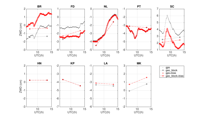
Figure 1: The residual zenith wet delay(ZWD) from GPS (black dots) and geodetic-block (black circles with dotted lines) data at nine VLBA stations during observations for program BZ039B. Corresponding red circles and red stars with dash-dotted lines are ZWDs with estimated biases removed as described in §4.

Figure 1 shows a comparison between the residual ZWDs from GPS and geodetic-block observations. The Owens Valley (OV) antenna did not participate in this session and the GPS ZTD products were not available for the Mauna Kea (MK) station. The ZWDs between the two geodetic-blocks are linear interpolations. The systematic biases between GPS and geodetic-block ZWD data (black markers in Figure 1) at stations FD and SC are about 2 cm, which are consistent with those reported by Zhang et al. (2008) and Honma et al. (2008).

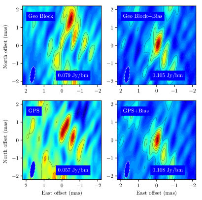
Figure 2: Phase-referenced images of J1820$-$2528 during the observation for program BZ039B, with geodetic-like observations (upper left panel), with geodetic-like observations plus bias correction (upper right panel), with GPS data (bottom left panel) and with GPS data plus bias correction (bottom right panel). Contour levels are spaced linearly at 15 mJy beam^-1.

The left panels of Figure 2 show the phase-referenced images of J1820$-$2528 made from data that had tropospheric delays calibrated with geodetic-block observations (top), with peak brightness of 79 mJy beam^-1, and GPS data (bottom), with peak brightness of 57 mJy beam^-1. (Note, that when calibrating data with the GPS method, for the four VLBA stations without GPS systems we substituted the geodetic-block estimates of wet zenith delay.) The images suggest that the ZWDs from the geodetic block calibration are better than for the GPS calibration. However, both images appear confused with several probable spurious components, indicating that there may still remain systematic errors with both methods. This motivated us to examine possible residual phase biases.

Two methods have been discussed in the literature to deal with residual phase biases and both involve a second-step calibration, either image optimization (Honma et al., 2008) or phase-fitting (Brunthaler et al., 2005). These calibrations work on the phase-referenced visibilities themselves, and are considered self-calibration methods, as opposed to GPS or geodetic block calibrations which use independent observations. Both self-calibration methods assume constant zenith delay-errors (biases) at each station over the observation period. The phase-fitting method is only appropriate for interferometer visibilities with high SNR, while the image optimization method can be applied to weak sources (Honma et al., 2008). Thus, we explored the image optimization approach here.

Following the process described in detail in § 4, we obtained a residual (total zenith) phase bias for each VLBA station that had been calibrated either by GPS data or geodetic blocks. Residual tropospheric ZWDs with phase biases removed are shown in Figure 1 with the red markers. The phase biases correspond to about 1 cm of path delay for most stations. The right panels in Figure 2 show the images of J1820$-$2528 with biases removed. Compared to the images without biases removed, the peak intensities increased from 79 to 105 mJy beam^-1 for geodetic-block calibration, and from 57 to 108 mJy beam^-1 for the GPS method. Figure 3 provides images from all four epochs for the different calibration methods. One can see that the bias-corrected images show simpler structure with a brighter dominant component than uncorrected images. We will discuss the improvement of astrometric accuracy with the bias correction in §5.

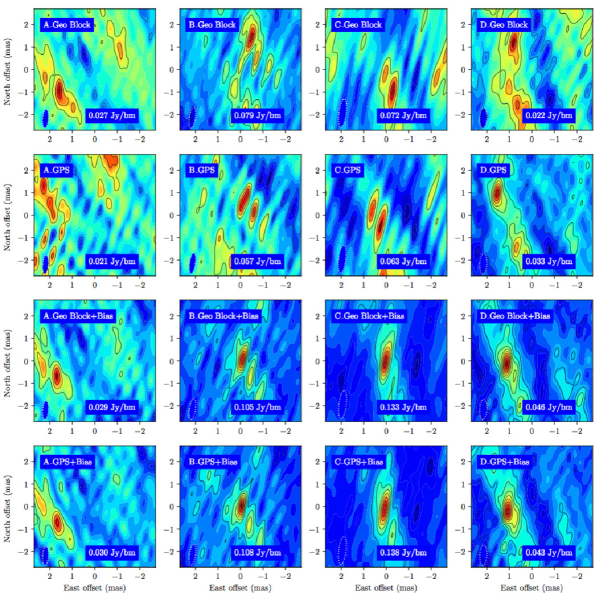
Figure 3: Phased-referenced image of J1820$-$2528  with different troposphere calibration methods. Panels from top to bottom are for calibrations with geodetic-blocks, GPS, geodetic-blocks with bias correction, and GPS with bias correction. Panels from left to right are for the VLBA program BZ039A, BZ039B, BZ039C and BZ039D, labeled with A, B, C and D, respectively. Contour levels are spaced linearly at 7 mJy beam^-1 (BZ039A), 15 mJy beam^-1 (BZ039B), 20 mJy beam^-1 (BZ039C) and 5 mJy beam^-1 (BZ039D) , respectively.

4 The method to obtain the bias

The image-optimization method for secondary calibration is described in Honma et al. (2008). The method essentially is a brute-force technique in which a grid of trial zenith delays are removed from the visibility data and subsequent maps are optimized for their peak brightnesses. The basic idea is that zenith delay errors degrade phase-referenced images, and the image with the greatest peak brightness should indicate the best zenith delay calibration.

As mentioned in §3, after primary calibration with either GPS data or geodetic blocks, residual zenith delay errors of 1 to 2 cm can exist. For our study, trial zenith path-delays for each antenna ranging from $\pm 3$ cm, with steps of between 0.2 to 0.5 cm, were removed from the data. The visibility data were then Fourier-transformed to make synthesized images, and the peak brightness is measured (without CLEAN deconvolution). In principle, it would be best to adjust residual biases simultaneously for all 10 VLBA antennas. But, this would be very time consuming, since even a 10 trial by 10 station grid would require constructing $10^{10}$ phase-referenced maps. Instead, we adjusted the trial zenith delays for one given antenna, holding the others constant, to achieve an optimal value for that antenna.

In our experience, the image-optimization method requires a reliable initial image. As shown in the left panel of Figure 4, after the geodetic-block calibration, the image made using data from all the stations shows several components. We cannot use the image-optimization method directly on such a poor image. Removing different stations from the uv database, we found that some stations degrade the image quality seriously (probably owing to large phase biases). After removing the problematic stations, the image showed one clear dominant component (see the middle panel of Figure 4). Next we used the image-optimization method based on this single component image to optimize the phase biases for the “clean” stations. After doing this, we introduced the “problem” stations one at a time and obtained preliminary phase biases for them. Finally, we iterated the procedure with all stations. The right panel of Figure 4 shows the finial image with the bias correction for all stations.

In order to assess the image optimization process, we examined the residual phases on each baseline. We shifted the source position so that the brightest component was near the map origin, which for perfect calibration should yield zero phases. Figure 5 shows these phases (green dots) for all VLBA baselines to the Kitt Peak (KP) station. The predicted phases based on the image optimization procedure (magenta dots for zenith phase shifts of BR = 1 cm, FD = 0.4 cm, LA = 0.2 cm, MK= 0.8 cm and SC = $-0.4$ cm) are also shown, as are residual differences (black dots). The BR and MK stations with the zenith phase biases of 1 cm show moderate phase residuals. The NL station residuals are quite large and systematic, possibly indicating that the assumption of a constant zenith bias is not valid here. Indeed, the ZWDs for NL changed by about 3 cm over the observations in BZ039B (see Fig. 1), the most for any station. Methods to address discrepant stations like NL remain to be developed.

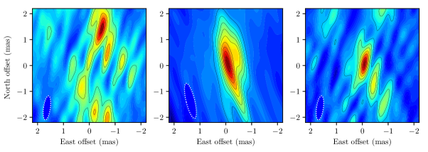
Figure 4: Phased-referenced images of J1820$-$2528  after the geodetic-block calibration for the VLBA program BZ039B. Left panel: using all stations. Middle panel: removing the BR, MK and NL stations. Right panel: using all stations after the bias correction. Contour levels are spaced linearly at 15 mJy beam^-1 .

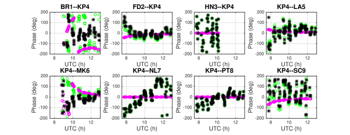
Figure 5: Interferometer phases for J1820$-$2528 for program BZ039B. Green dots: data using the geodetic-block calibration; magenta dots: model phases based on zenith biases; black dots: residual phases after bias correction.

5 Parallax and Proper Motion

Figure 6 shows the interferometer spectra of H₂O maser emission observed with one VLBA baseline at all four epochs. The H₂O maser emission spans a $V_{\rm LSR}$ range from about –15 to 25 km s^-1. The flux densities of maser features between $V_{\rm LSR}$ of 0 and 10 km s^-1 varied considerably from epoch to epoch, while the peaks of blue-shifted ($V_{\rm LSR}$ $\approx-10$ km s^-1) and red-shifted ($V_{\rm LSR}$  $\approx 20$ km s^-1) features were more stable. The systemic velocity of VX Sgr is estimated to be 5 km s^-1, based on a dynamical model of an expanding envelope fitted to interferometric maps of OH maser emission at 1612 MHz (Chapman & Cohen, 1986). Figure 7 shows the spatial distribution of H₂O maser emission toward VX Sgr relative to the reference maser spot at $V_{\rm LSR}$ = 1.2 km s^-1 from observations at one of the epochs. We found 16 maser spots detected at all epochs that could be used for precision astrometry. In Figure 7, these maser spots cluster in eight locations identified with letters A through H in velocity order.

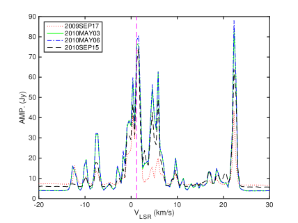
Figure 6: Interferometer spectra (scalar averaged cross-power amplitude over the full duration of the observation) of the H₂O masers toward VX Sgr from Kitt Peak to Los Alamos baseline at four epochs. The red dashed line indicates the maser feature at VLSR of $V_{\rm LSR}$ = 1.2 km s^-1 which served as the interferometer phase reference.

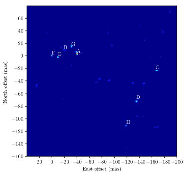
Figure 7: Spatial distribution of the velocity integrated H₂O maser features toward VX Sgr from VLBA observations on 2009 September 17.

Figure 8 shows the maser reference channel images at all four epochs. One can see that the emission appears dominated by a single compact component. Fifteen other maser spots were compact, and we fitted elliptical Gaussian brightness distributions to these masers and the extragalactic radio source J1820$-$2528 for all four epochs. (The extragalactic source J1808$-$2124 was not detected in our observations.) The change in position of each maser spot relative to J1820$-$2528 was modeled by the parallax sinusoid in both coordinates and a linear proper motion in each coordinate.

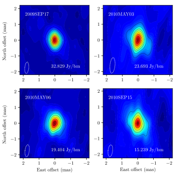
Figure 8: Images of the phase reference H₂O maser spot at $V_{\rm LSR}$ = 1.2 km s^-1 toward VX Sgr at four epochs. The restoring beam is indicated in the lower left corner of each panel. Contour levels are spaced linearly at 3.0 Jy beam^-1.

We compared the astrometry results using the different methods to calibrate residual tropospheric delays as discussed in §3. Table 3 shows the parallax and proper motion fits for the reference maser spot with different troposphere calibration methods. All parallaxes are consistent within their joint uncertainties. However, when the secondary calibration to remove phase bias is applied, the parallax uncertainties decrease by about a factor of two. While parallax uncertainties from four epochs, a single background source, and dominated by the East-West offsets are themselves quite uncertain (Reid et al., 2017), this comparison is based on the same data with only a single calibration difference and should be significant. In addition, as shown in the Figure 2, the quality of the phase-referenced quasar images improved significantly with phase bias corrections, providing strong evidence for the validity of this secondary calibration.

Table 3: Parallax and proper motion fits for the reference maser spot

Methods	Parallax	Distance	$\mu_{x}$	$\mu_{y}$
	(mas)	(kpc)	(mas yr-1)	(mas yr-1)
geodetic blocks	0.70 $\pm$ 0.09	1.44 $\pm$ 0.13	0.59 $\pm$ 0.20	-0.95 $\pm$ 0.34
GPS	0.56 $\pm$ 0.11	1.78 $\pm$ 0.20	1.42 $\pm$ 0.27	1.81 $\pm$ 1.56
geodetic blocks+bias	0.66 $\pm$ 0.05	1.51 $\pm$ 0.07	0.62 $\pm$ 0.10	-0.97 $\pm$ 0.25
GPS+bias	0.69 $\pm$ 0.05	1.45 $\pm$ 0.07	0.70 $\pm$ 0.15	-0.69 $\pm$ 0.51

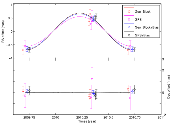
Figure 9: Parallax and proper motion data and best-fitting models for the reference maser spot at $V_{\rm LSR}$ of 1.2 km s^-1 with different troposphere calibration methods. Data for the maser spots with different methods are offset horizontally for clarity.

Since one expects the same parallax for all maser spots, we did a combined solution (fitting with a single parallax parameter for more maser spots, but allowing for different proper motions for each maser spot) using 16 bright maser spots. Table 4 shows the independent and combined parallax fits for those maser spots. The combined parallax estimate for the geodetic block plus bias corrected data is $0.64\pm 0.04$ mas, corresponding to a distance of $1.56^{+0.11}_{-0.10}$ kpc. The quoted uncertainty is the formal error multiplied by $\sqrt{16}$ to allow for the liklihood of correlated position variations for the 16 maser spots. This could result from small variations in the background source or from mismodeled atmospheric delays, both of which would affect the maser spots identically (Reid et al., 2009).

Table 4: Parallax and proper motion fits for VX Sgr 

Region	Ch.	$V_{\rm LSR}$	Parallax	$\mu_{x}$	$\mu_{y}$	dx	dy
		(km s-1)	(mas)	(mas yr-1)	(mas yr-1)	(mas)	(mas)
A	87	22.6	0.623 $\pm$ 0.056	0.58 $\pm$ 0.14	-0.32 $\pm$ 0.32	-41.17 $\pm$ 0.05	3.84 $\pm$ 0.11
A	89	21.8	0.668 $\pm$ 0.025	0.27 $\pm$ 0.07	-1.02 $\pm$ 0.23	-41.11 $\pm$ 0.02	3.18 $\pm$ 0.08
B	118	9.6	0.615 $\pm$ 0.065	0.68 $\pm$ 0.16	-0.95 $\pm$ 0.25	-20.01 $\pm$ 0.06	9.79 $\pm$ 0.09
B	119	9.2	0.657 $\pm$ 0.039	0.59 $\pm$ 0.10	-1.07 $\pm$ 0.54	-20.61 $\pm$ 0.03	9.18 $\pm$ 0.20
C	127	5.8	0.694 $\pm$ 0.091	-1.65 $\pm$ 0.22	-1.89 $\pm$ 0.21	-168.01 $\pm$ 0.08	-23.29 $\pm$ 0.07
D	129	4.9	0.624 $\pm$ 0.046	-1.41 $\pm$ 0.12	-2.98 $\pm$ 0.32	-135.75 $\pm$ 0.04	-72.10 $\pm$ 0.12
D	130	4.5	0.653 $\pm$ 0.041	-1.52 $\pm$ 0.10	-3.08 $\pm$ 0.38	-135.87 $\pm$ 0.04	-71.34 $\pm$ 0.14
D	131	4.1	0.562 $\pm$ 0.017	-1.28 $\pm$ 0.05	-2.81 $\pm$ 0.34	-136.83 $\pm$ 0.02	-71.08 $\pm$ 0.13
E	137	1.6	0.579 $\pm$ 0.037	0.56 $\pm$ 0.09	-1.11 $\pm$ 0.34	-10.29 $\pm$ 0.03	-1.96 $\pm$ 0.12
F	138	1.2	0.650 $\pm$ 0.031	0.65 $\pm$ 0.08	-0.97 $\pm$ 0.28	-0.66 $\pm$ 0.03	0.18 $\pm$ 0.10
F	139	0.7	0.644 $\pm$ 0.040	0.69 $\pm$ 0.10	-0.90 $\pm$ 0.25	-0.55 $\pm$ 0.04	0.31 $\pm$ 0.09
G	140	0.3	0.655 $\pm$ 0.036	-0.01 $\pm$ 0.09	-0.82 $\pm$ 0.38	-32.11 $\pm$ 0.03	14.67 $\pm$ 0.14
G	142	-0.4	0.633 $\pm$ 0.037	0.06 $\pm$ 0.09	-0.78 $\pm$ 0.40	-31.44 $\pm$ 0.03	16.35 $\pm$ 0.15
H	158	-7.2	0.650 $\pm$ 0.027	-1.55 $\pm$ 0.07	-3.51 $\pm$ 0.35	-118.98 $\pm$ 0.03	-110.44 $\pm$ 0.13
H	159	-7.6	0.656 $\pm$ 0.014	-1.48 $\pm$ 0.04	-3.50 $\pm$ 0.37	-119.02 $\pm$ 0.01	-110.69 $\pm$ 0.14
H	160	-8.0	0.648 $\pm$ 0.015	-1.50 $\pm$ 0.04	-3.56 $\pm$ 0.36	-119.05 $\pm$ 0.02	-110.87 $\pm$ 0.13
Combined			0.639 $\pm$ 0.042

We measured the absolute proper motion of the reference maser spot ( $V_{\rm LSR}$  = 1.2 km s^-1 ) to be $\mu_{x}$  = $0.65\pm 0.08$ mas yr^-1  and $\mu_{y}$  = $-0.97\pm 0.28$ mas yr^-1. In order to model the internal motions of the masers to obtain the absolute proper motion of the central star of VX Sgr, we used the 16 maser spots that appeared at four epochs within one year, and estimated their motions with respect to the reference maser spot. We fitted the data to a model of an expanding outflow. The estimated parameters are from a Bayesian fitting procedure described by Sato et al. (2010). Converting the systematic velocity of expanding outflow center (central star) of $(V_{0x}$ = -2.19 $\pm$ 5.69 km s^-1, $V_{0y}$ = -14.50 $\pm$ 5.44 km s^-1, $V_{0r}$ = 6.47 $\pm$ 3.37 km s^-1) to angular motions yields $\mu_{x}$ = -0.29 $\pm$ 0.76 mas yr^-1 and $\mu_{y}$ = -1.95 $\pm$ 0.73 mas yr^-1 at the distance of 1.56 kpc to VX Sgr. Adding this motion to the absolute motion of the reference maser spot, we estimate an absolute proper motion of VX Sgr to be $\mu_{x}$ = 0.36 $\pm$ 0.76 mas yr^-1 and $\mu_{y}$ = –2.92 $\pm$ 0.78 mas yr^-1. We note that while the $Hipparcos$ parallax (3.82 $\pm$ 2.73 mas) and eastward proper motion ($\mu_{x}$ = $3.20\pm 3.08$ mas yr^-1) have large uncertainties and allow no meaningful comparison with our results, their northward motion ($\mu_{y}$ = $-6.71\pm 1.72$ mas yr^-1, van Leeuwen (2007)) differs from our much more accurate result by more than $2\sigma$. This discrepancy might be associated with inhomogeneities and dust scattering the optical light in the circumstellar envelope (Zhang et al., 2012a).

Figure 10 compares our astrometric results of VX Sgr with 22 of the brightest stars in the Sgr OB1 association (Humphreys, 1978). Our measured astrometric results are in excellent agreement these cluster members and confirm that VX Sgr belongs to the Sgr OB1 association.

Chiavassa et al. (2010) estimated the bolometric luminosity of VX Sgr is $L_{\rm bol}$ = $(0.73\pm 0.38)\times 10^{5}$ $(d/{\rm kpc})^{2}~{}L_{\odot}$, adopting an effective temperature of 3200 to 3400 K. This luminosity is in good agreement with that $L_{\rm bol}$ = $(0.67\pm 0.18)\times 10^{5}$ $(d/{\rm kpc})^{2}~{}L_{\odot}$  estimated by Lockwood & Wing (1982), from a measured magnitude at 10400 Å and applying a bolometric correction. However, Mauron & Josselin (2011) determined a maximum luminosity (without a quoted uncertainty) of $L_{\rm bol}$ = $1.38\times 10^{5}$ $(d/{\rm kpc})^{2}~{}L_{\odot}$, by integrating UBVIJHKL + IRAS photometry. De Beck et al. (2010) derived $L_{\rm bol}$ = $0.42\times 10^{5}$ $(d/{\rm kpc})^{2}~{}L_{\odot}$, assuming the K-band magnitude is a function of pulsation period and effective temperature. Combined these estimated luminosity, we recalculate $L_{\rm bol}$ = $(0.80\pm 0.23)\times 10^{5}$ $(d/{\rm kpc})^{2}~{}L_{\odot}$  using an un-weighted average and standard error of the mean (SEM) estimate, corresponding to $(1.95\pm 0.62)\times 10^{5}$ $L_{\odot}$  by adopting our parallax distance of $1.56^{+0.11}_{-0.10}$ kpc. This luminosity coupled with an effective temperature of 3300 K suggests a radius for VX Sgr of 1,120 to 1,550 $R_{\odot}$.

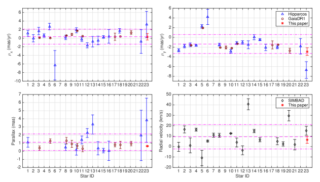
Figure 10: Proper motion, parallax and radial velocity results in Sgr OB1 association. The star ID from 1 to 23 stands for HD 163428, HD 163800, HD 163892, HD 164402, HD 164438, HD 164492, HD 164514, HD 164794, HD 164816, HD 165052, HD 165516, HD 165784, HD 166167, HD 166546, HD 166937, HD 163777, HD 164018, HD 164637, HD 164883, HD 164906, HD 165285, HD 166524 and VX Sgr, respectively. The proper motion and parallax results are from $Hipparcos$ (van Leeuwen, 2007), Gaia DR1 (Gaia Collaboration et al., 2016) and this paper. The radial velocity results from the SIMBAD astronomical database (Wenger et al., 2000) are converted from heliocentric frame to the local standard of rest. The horizontal dashed magenta lines indicate the means and the dash-dotted lines indicate the mean $\pm$ 1 standard deviation with the unweighted estimation for the results in Sgr OB1 association.

6 FUTURE OUTLOOK

We have shown that for our data set there are systematic biases of $\approx 1$ cm of tropospheric zenith path-delay between GPS and VLBI geodetic block calibrations. These biases can be estimated by an image-optimization method and we find the primary calibration via geodetic block is slightly better than GPS method. Even small residual biases of $\approx 1$ cm of zenith path delay can degrade image quality and astrometric accuracy when low source elevation data are used. Therefore, correction of tropospheric phase-delay biases can be important for a very accurate parallax measurements. The combination of image-optimization and additional geodetic VLBI blocks or GPS measurements of ZWD is an effective way to accomplish this. This method might be of great benefit when applied to archival VLBI data taken before geodetic block calibrations were standard.

References

- Asaki et al. (2010) Asaki, Y., Deguchi, S., Imai, H., et al. 2010, ApJ, 721, 267
- Brunthaler et al. (2005) Brunthaler, A., Reid, M. J., & Falcke, H. 2005, in Astronomical Society of the Pacific Conference Series, Vol. 340, Future Directions in High Resolution Astronomy, ed. J. Romney & M. Reid, 455
- Chapman & Cohen (1986) Chapman, J. M., & Cohen, R. J. 1986, MNRAS, 220, 513
- Chen et al. (2007) Chen, X., Shen, Z.-Q., & Xu, Y. 2007, Chinese J. Astron. Astrophys., 7, 531
- Chiavassa et al. (2010) Chiavassa, A., Lacour, S., Millour, F., et al. 2010, A&A, 511, A51
- Choi et al. (2008) Choi, Y. K., Hirota, T., Honma, M., et al. 2008, PASJ, 60, 1007
- De Beck et al. (2010) De Beck, E., Decin, L., de Koter, A., et al. 2010, A&A, 523, A18
- Deller et al. (2007) Deller, A. T., Tingay, S. J., Bailes, M., & West, C. 2007, PASP, 119, 318
- Gaia Collaboration et al. (2016) Gaia Collaboration, Brown, A. G. A., Vallenari, A., et al. 2016, A&A, 595, A2
- Honma et al. (2008) Honma, M., Tamura, Y., & Reid, M. J. 2008, PASJ, 60, 951
- Humphreys (1978) Humphreys, R. M. 1978, ApJS, 38, 309
- Lockwood & Wing (1982) Lockwood, G. W., & Wing, R. F. 1982, MNRAS, 198, 385
- Ma et al. (1998) Ma, C., Arias, E. F., Eubanks, T. M., et al. 1998, AJ, 116, 516
- Mauron & Josselin (2011) Mauron, N., & Josselin, E. 2011, A&A, 526, A156
- Ning et al. (2012) Ning, T., Haas, R., Elgered, G., & Willén, U. 2012, Journal of Geodesy, 86, 565
- Pradel et al. (2006) Pradel, N., Charlot, P., & Lestrade, J.-F. 2006, A&A, 452, 1099
- Reid & Honma (2014) Reid, M. J., & Honma, M. 2014, ARA&A, 52, 339
- Reid et al. (2009) Reid, M. J., Menten, K. M., Brunthaler, A., et al. 2009, ApJ, 693, 397
- Reid et al. (1999) Reid, M. J., Readhead, A. C. S., Vermeulen, R. C., & Treuhaft, R. N. 1999, ApJ, 524, 816
- Reid et al. (2017) Reid, M. J., Brunthaler, A., Menten, K. M., et al. 2017, AJ, 154, 63
- Samus’ et al. (2017) Samus’, N. N., Kazarovets, E. V., Durlevich, O. V., Kireeva, N. N., & Pastukhova, E. N. 2017, Astronomy Reports, 61, 80
- Sato et al. (2010) Sato, M., Reid, M. J., Brunthaler, A., & Menten, K. M. 2010, ApJ, 720, 1055
- Steigenberger et al. (2007) Steigenberger, P., Tesmer, V., Krügel, M., et al. 2007, Journal of Geodesy, 81, 503
- Teke et al. (2013) Teke, K., Nilsson, T., Böhm, J., et al. 2013, Journal of Geodesy, 87, 981
- van Leeuwen (2007) van Leeuwen, F. 2007, A&A, 474, 653
- van Moorsel et al. (1996) van Moorsel, G., Kemball, A., & Greisen, E. 1996, in Astronomical Society of the Pacific Conference Series, Vol. 101, Astronomical Data Analysis Software and Systems V, ed. G. H. Jacoby & J. Barnes, 37
- Wenger et al. (2000) Wenger, M., Ochsenbein, F., Egret, D., et al. 2000, A&AS, 143, 9
- Zhang et al. (2012a) Zhang, B., Reid, M. J., Menten, K. M., & Zheng, X. W. 2012a, ApJ, 744, 23
- Zhang et al. (2012b) Zhang, B., Reid, M. J., Menten, K. M., Zheng, X. W., & Brunthaler, A. 2012b, A&A, 544, A42
- Zhang et al. (2008) Zhang, B., Zheng, X.-W., Li, J.-L., & Xu, Y. 2008, Chinese J. Astron. Astrophys., 8, 127