A spline-assisted semiparametric approach to nonparametric measurement error models
Fei Jiang
Department of Statistics, University of Hongkong, Hongkong
feijiang@hku.hk
and
Yanyuan Ma
Department of Statistics, Penn State University, University Park, PA 16802
yzm63@psu.edu
and
Raymond J. Carroll
Department of Statistics, Texas A&M University, College Station TX and
School of Mathematical and Physical Sciences, University of Technology Sydney, Broadway NSW 2007, Australia
carroll@stat.tamu.edu
Abstract
It is well known that the minimax rates of convergence of nonparametric density and regression function estimation of a random variable measured with error is much slower than the rate in the error free case. Surprisingly, we show that if one is willing to impose a relatively mild assumption in requiring that the error-prone variable has a compact support, then the results can be greatly improved. We describe new and constructive methods to take full advantage of the compact support assumption via spline-assisted semiparametric methods. We further prove that the new estimator achieves the usual nonparametric rate in estimating both the density and regression functions as if there were no measurement error. The proof involves linear and bilinear operator theories, semiparametric theory, asymptotic analysis regarding Bsplines, as well as integral equation treatments. The performance of the new methods is demonstrated through several simulations and a data example.
Keywords: Errors in covariates, measurement error, semiparametrics, spline.
1 Introduction
Density estimation is a familiar problem in the nonparametric estimation literature. Generally, we observe independent and identically distributed variables from a distribution with probability density function (pdf) and nonparametric estimators such as kernel methods are available in the literature to estimate . Even when the ’s are not directly observed, nonparametric estimation of can still be carried out based on their surrogates. Specifically, assume that instead of observing , we observe , where is a mean zero random error independent of and follows a distribution with pdf . This problem has been studied extensively in the literature (Carroll & Hall, 1988; Liu & Taylor, 1989; Stefanski & Carroll, 1990; Zhang, 1990; Fan, 1991) and it is well known that the estimator of may converge very slowly. For example, when the error distribution is normal or within the class of “super smooth” distributions, an estimator can only converge to at the rate of where is a positive constant. When the error distribution is Laplace or another “ordinary smooth” type, the convergence rate is , where is a positive constant smaller than 0.25. Here “super smooth” and “ordinary smooth” are characteristics well explained in, for example, Fan (1991). These convergence rates are minimax for general . When the ’s are observed, nonparametric density estimation usually performs much better than these results. We describe a simple constraint that allows rates of convergence that are much faster than the minimax rates, and achieves the same rate as when there is no measurement error.
A problem parallel to nonparametric density estimation is nonparametric regression. Likewise, when observations , , are available, many nonparametric estimators such as kernel and spline based methods have been proposed to estimate the regression mean of conditional on . Here the assumption is that , where for simplicity, we assume is independent of and has mean zero with density . When is unavailable and instead only described above is available, we encounter the problem of nonparametric regression with measurement error. It is also well established (Fan & Truong, 1993) that the same possibly slow rate of convergence occurs as in the density estimation case. These convergence rates are also minimax, and again, with a simple constraint, we can very nearly achieve the non-measurement error rates.
Working within the Bspline framework, the constraint mentioned above is that the support of the latent is compact. This constraint also arises the in the work of Hall & Qiu (2005), although they did not use a Bspline approach. Since a Bspline representation of a function is typically done on a compact support, we use Bspline assisted methods.
Using spline representation in measurement error models is not entirely new, although it was mostly used in the Bayesian framework (Berry et al., 2002; Staudenmayer et al., 2008; Sarkar et al., 2014). While the density estimator is relatively easy to devise, see Staudenmayer et al. (2008), regression estimation turns out to be challenging and it most convenient with our novel further semiparametric treatment. A second challenge in both problems is in establishing the convergence rates of the resulting estimators. The common obstacle in both estimators is the fact that it is a latent function that needs to be approximated with a spline representation, which requires unusual treatment different from the typical handling of the spline approximation. In addition, for the regression problem, we encounter further difficulties because not only the estimator, but also the estimating equation that generates the estimator, do not have closed forms. We have made novel use of bilinear operators (Conway, 1990), which are very different from typical regression spline asymptotic analysis (Ma et al., 2015). The detailed proofs are in the Appendix and in an online Supplement.
In the Bspline approximation, the compact set on which we perform the estimation is built into the procedure at the very beginning and we benefit from that throughout the procedure. Classically, deconvolution is the most widely used method in nonparametric measurement error problems. In the typical deconvolution procedures, the Fourier and inverse Fourier transformation steps do not take advantage of the compact set knowledge. Instead, it automatically estimates these functions on the whole interval, which is much harder to do. How to modify the deconvolution procedures to make use of the compact support of is an interesting future research topic and is well worth exploring.
In the following, we construct the estimation procedures for both the probability density function and the regression mean function in Section 2, and summarize the theoretical properties of our estimators in Section 3. We provide simulation studies to demonstrate the properties of the new estimators in Section 4, and illustrate the methods in a data example in Section 5. The paper is concluded with a discussion in Section 6.
2 Bspline-assisted estimation procedures
2.1 Probability density function estimation
To set the notation, we use to denote a generic pdf function of the random variable , and use to denote the true pdf that generates the data. We approximate on its support using Bsplines (Masri & Redner, 2005). For simplicity, let the support be . To ensure that the density function is nonnegative and integrates to 1, we let the approximation be
| (1) |
where is a vector of Bspline basis functions, and is the Bspline coefficient vector. For reasons of identifiability, we fix the first component of at zero, i.e. , and leave the remaining components free. Here, denotes the subvector of a generic vector without the first element. This is different from the estimator of Staudenmayer et al. (2008). Then
is an approximation to the pdf of , a surrogate of . We then perform simple maximum likelihood estimation (MLE), i.e. we maximize
with respect to to obtain , and then reconstruct and use it as the estimator for , i.e. . Here .
While the estimation procedure for is extremely simple, it is not as straightforward to establish the large sample properties of the estimator. In Section 3, we will show that converges to at a near-nonparametric rate under mild conditions.
2.2 Regression function estimation
Unlike in the density estimation case, the estimation procedure in the regression model is much more complex. Without considering that the number of basis functions will increase with sample size, the key observation is that as soon as the nonparametric function is approximated with the Bspline representation, the regression function itself without measurement error is a purely parametric model (Wang & Yang, 2009), hence the idea behind Tsiatis & Ma (2004) can be adapted. Specifically, we treat the Bspline coefficients as parameters of interest, treat the unspecified distribution of , , as nuisance parameter, and cast the problem as a semiparametric estimation problem. We can then construct the efficient score function, which relies on . A key observation of Tsiatis & Ma (2004) is that by replacing with an arbitrary working model, the consistency of estimation is retained. We now describe the estimation procedure in detail.
First, let be a working pdf of . Of course, may not be the same as , that is, is possibly misspecified. Following the practice of density estimation in Section 2.1, assume that the true density function has compact support . Therefore we only need to consider on . We approximate using the spline representation . Define
As the notation suggests, is the score function with respect to calculated from the joint pdf of under the working model and the spline approximation. Due to the possible misspecification of , the mean of is not necessarily zero even if the mean function is exactly . Therefore simply solving may generate an inconsistent estimator. The idea behind our estimator is to find a function so that
and then solve for using the estimating equation
| (3) | |||
This will guarantee a consistent estimator of if the mean function is indeed , because our construction ensures the left hand side of (3) has mean zero. The right hand side of (2.2) is the conditional expectation of calculated under the Bspline approximation and the posited model , hence we alternatively write it as .
To solve for , we discretize the integral equation (2.2). In particular, let , where ’s are points selected on , and . Then
Next, to write out the right hand side of (2.2) upon discretization, let be an matrix with its entry
Let , . Further, define , where
and let be a matrix, with its th column
Then .
With this notation, the integral equation (2.2) is equivalently written as for , or more concisely, . Therefore
hence
where is a length vector with the th component 1 and all others zero.
Thus, we have obtained on the discrete set and can form
where
We then obtain the estimator for by solving the estimating equation (3) with the corresponding plugged in. In all the functions that are explicitly written to depend on , the dependence is always through .
We show that converges to at a nonparametric rate and we derive its estimation variance in Section 3 under mild conditions. Instead of adopting a working model , we could in fact estimate using the method developed in Section 2.1 to obtain , and then use instead of to carry out the subsequent operations. Although this is the optimal thing to do in theory, we find the practical improvement of estimation efficiency very small. In addition, unless the sample size is very large, numerical instability can arise and sometimes does so. For these reasons, we do not recommend this approach.
3 Asymptotic results
3.1 Results of probability density function estimation
We assume the following regularity conditions.
-
(C1)
The true density function has compact support , is bounded and positive on its support and satisfies , . The error density is bounded. The conditional density of given , , is bounded.
-
(C2)
The spline order .
-
(C3)
Define the knots , where is the number of interior knots and is divided into subintervals. Let . satisfies , when .
-
(C4)
Let be the distance between the st and th interior knots and let , . There exists a constant , , such that
Therefore, , .
-
(C5)
is a spline coefficient with first component such that , where is defined in (1).
Remark 1.
exists because by De Boor (1978) there is a such that . Then satisfies the condition, where is a vector of ones. The argument is facilitated by the fact that .
-
(C6)
The expectation
is a smooth function of and has unique root in the neighborhood of .
Condition (C1) contains some basic boundedness and smoothness conditions on various densities and is quite standard. The only requirement that appears nonstandard is that has compact support. This however is practically relevant in many situations as the range of the values a random variable can be may very well be bounded. Condition (C2) is a standard requirement to ensure that splines of sufficiently high order are utilized. Condition (C3) requires a suitable amount of spline basis to be used according to the sample size, and Condition (C4) makes sure that the spline knots are distributed sufficiently evenly. In summary, Conditions (C2), (C3) and (C4) are standard requirements and together with Condition (C1), they ensure Condition (C5). We list Condition (C5) instead of stating it in the proof for convenience. Finally, Condition (C6) ensures that we are not in the degenerate case where the expression in (C6) is constantly zero. Under these conditions, we obtain the following properties of .
Proposition 2.
Propositions 1 and 2 establishes the consistency and convergence rate properties of to defined in Condition (C5). The proof of Propositions 1 and 2 are in Supplement LABEL:sec:appconsist and LABEL:sec:apptheta, respectively. We then utilize these properties to analyze the bias, variance and convergence rate of in Theorem 1, with its proof in Appendix A.1.
Theorem 1.
Theorem 1 shows that the Bspline MLE density estimator has bias of order and standard error of order , which is the standard nonparametric density estimation result when no measurement error occurs, and is a substantial improvement compared to the minimax convergence rate without the compact support assumption. In addition, to minimize the MSE, we can use , leading to the MSE with order . On the other hand, to suppress the estimation bias asymptotically, we need to under-smooth by setting .
3.2 Results of regression mean function estimation
To facilitate the description of the regularity conditions and the asymptotic results, we introduce some notation. Define
and write
We further define , , , to be the resulting quantities when we replace all the appearance of in , , , and by respectively. Here is a function that satisfies
where the last is used to emphasize that the calculation of the outside expectation depends on . These definitions do not conflict with the notation used before. In fact, some generalize the previous notation. We further define to be a linear operator on whose value at is
The derivative of is a bilinear operator on with , whose value at is
Further, we define a bilinear operator
From the above definition,
Also,
where and
.
We now list the regularity conditions.
-
(D1)
The true density functions are bounded on their supports. In addition, the support of is compact.
-
(D2)
is a bounded bilinear operator on , , and . Also, is a bounded bilinear operator on .
-
(D3)
is bounded on and it satisfies , .
-
(D4)
is a dimensional spline coefficient such that . The existence of such has been shown in De Boor (1978).
-
(D5)
The expectation
has a unique root for in the neighborhood of . Its derivative with respect to is a smooth function of in the neighborhood of , with its singular values bounded and bounded away from zero. Denote the unique zero as .
Conditions (D1) and (D2) contain boundedness requirements on pdfs and operators and are not stringent. Condition (D1) further requires the compact support of the distribution of . This is similar to the density estimation case and is crucial. Conditions (D3) and (D4) are regarding the mean function and its spline approximation which are quite standard. Condition (D5) is a unique root requirement similar to (C6) and is used to exclude the pathologic case where the estimating equation is constantly zero.
In the following, we establish the consistency of the parameter estimation in Proposition 3 and then further analyze its convergence rate in Proposition 4. The results in these propositions are subsequently used to further establish the asymptotic properties of the estimator of the regression mean function in Theorem 2. The proofs of both the propositions and the theorem are in Supplement LABEL:sec:appbetaconsis, LABEL:sec:appbeta and Appendix A.2 respectively.
Theorem 2.
Theorem 2 shows that the Bspline regression mean function estimator has bias of order and standard error of order , which is the standard nonparametric regression result without measurement error, and is much better than the minimax convergence rate without assuming to be compactly supported. Further, to minimize the MSE, we let , leading to the MSE of order . On the other hand, to suppress the estimation bias asymptotically, we need to under-smooth by setting .
4 Simulation studies
4.1 Performance of the Bspline-assisted density estimator
We conducted two simulation studies to illustrate the finite sample performance of the proposed pdf and regression mean estimators. To evaluate the Bspline MLE method for estimating the density functions, we generated data sets of sample sizes from to . We used cubic Bsplines with the number of knots equal to the smallest integer larger than . In all our simulations, is generated from a beta distribution with both shape parameters equal to 4. We then generated the measurement error from three models:
-
I(a): a normal distribution with mean 0, variance , denoted by ,
-
I(b): a Laplace distribution with mean 0 and scale , denoted by ,
-
I(c): a uniform distribution on , denoted by
.
In the left panel of Figure 1, we plotted the averaged root- maximum absolute error (MAE), calculated as , versus the sample sizes . Following Theorem 1, the root- MAE has a constant order.
This translates to the curves in the plots that stabilize in a small range, which is what we observe, especially when the sample size grows to larger than 700.
We also compared the Bspline MLE method with the widely used deconvolution method (Stefanski & Carroll, 1990) for density estimation that does not assume is compactly supported. In the upper row of Figure 2, we plotted the average values of based on 200 simulations for both methods at different sample sizes. We adopted the two-stage plug-in bandwidth selection method proposed in Delaigle & Gijbels (2002) in implementing the deconvolution method. Unsurprisingly, results in the upper row of Figure 2 indicate that the Bspline MLE method outperforms the deconvolution method with rather significant gain in this case. We suspect that this is because the measurement errors are quite large here which caused difficulties for both methods, but especially for the deconvolution method.
To further examine the performance of individual estimated pdf curves from both methods, we also plotted the estimated mean density curves for sample sizes 500, 1000 and 2000. Because the deconvolution method performs poorly when the measurement errors are large (see upper row of Figure 2), we reduced the error variances, and generated the three error distributions from models
-
II(a): , II(b): , II(c): .
Under the reduced error variability, we performed the estimation and plotted the resulting density estimates and their 90% confidence bands. Figure 3 contains the results of the Bspline MLE and the deconvolution estimator using the two-stage plug-in bandwidth (Delaigle & Gijbels, 2002), at the sample size 500. Although not as dramatic as the large error case, the Bspline MLE is still closer to the true pdf with narrower confidence band, hence is more precise than the deconvolution method.
We also provide similar comparisons at sample sizes 1000 and 2000 in Figures LABEL:fig:den2 and LABEL:fig:den3 in the Supplement. For a quantitative comparison, we also computed the MAE between the true pdf curve and the estimated pdf curve in the upper part of Table 1. These results show that the Bspline MLE performs consistently better than deconvolution which does not make the compact support assumption. The performance of the two methods largely follow the same pattern when sample sizes are smaller, although the improvement of the Bspline method over the deconvolution method is not as dramatic, naturally. We provide the results for in Figure LABEL:fig:den0 in the Supplement.
4.2 Performance of the Bspline-assisted semiparametric estimator
We next evaluated the finite sample performance of the Bspline semiparametric mean regression method described in Section 2.2. We used sample sizes from 500 to 2000, used cubic Bsplines, with the number of knots equal to the smallest integer larger than . In this case we generated from a beta distribution with both shape parameters equal to 2. The true regression mean function is and we generated the regression model errors from a normal distribution with mean zero and variance 0.25. We generated the measurement errors from the three different distributions described in Models I(a)–I(c).
In the right panel of Figure 1, we plotted the averaged root- MAE calculated via as a function of the sample size . Similar to the density estimation experiment, the curves stabilize as sample size increases, and is largely flat after , indicating that has order .
We further compared the Bspline semiparametric method with the deconvolution method (Fan & Truong, 1993) in the nonparametric mean regression model, where the deconvolution method does not make the compact support assumption on . In the lower row of Figure 2, we plotted the average over 200 simulations for both methods. Again, in this case, with moderate to significant amount of noise, the Bspline semiparametric method greatly outperforms the deconvolution method with smaller average error.
Similar to the pdf investigation, we reduced the measurement error variability and generated the errors from model II (a)–(c) to investigate the mean function curve fitting. We plotted the mean function estimates and the 90% confidence bands for the Bspline semiparametric and deconvolution methods in Figure 4 for sample size 500, and also provided the same results in Figures LABEL:fig:mean2, LABEL:fig:mean3 and LABEL:fig:mean0 in the Supplement. for sample sizes 1000, 2000, as well as 200. These results indicate that the Bspline semiparametric estimator indeed outperforms the deconvolution method, which does not make a compact support assumption on . Their performance difference in terms of averaged MAE between the estimated and true mean curves are further provided in the lower half of Table 1. The deconvolution density estimation and nonparametric regression are implemented using the code from the website https://researchers.ms.unimelb.edu.au/aurored/links.html.
5 Data example
Heavy fine particulate matter (PM2.5) air pollution has become a serious problem in China and its possible effect on respiratory diseases has been a concern in public health. Starting from 2012, the Beijing Environmental Protection Bureau (BEPB) has been recording the daily PM2.5 levels in Beijing. Based on these data, Xu et al. (2016) studied the effect of PM2.5 on asthma in 2013. Specifically, they explored the PM2.5 effect on the number of daily asthma emergency room visits (ERV) in ten hospitals in Beijing, but found no significant effect. In fact, the mean number of daily asthma ERVs even shows a decreasing trend along the increase of measured PM2.5. This contradicts the general conclusion that PM2.5 has short term adverse effect on asthma (Fan et al., 2016).
A potential reason of this inconsistency is the errors in the PM2.5 measurements which were not taken into account in the above analysis. In fact, there are many debates on the accuracy of the PM2.5 reports, especially in the early years such as 2013. For example, we compared the daily average PM2.5 reports in 2013 from 17 ambient air quality monitoring stations and those reports from the “Mission China Beijing” website (Mission-China, 2016) maintained by the U.S. Department of State, and show the two estimated pdfs of PM2.5 in Figure 5. It is clear that the estimated pdfs of PM2.5 from the two sources are very different, where the PM2.5 concentrations obtained from the BEPB yields a pdf estimate with the mode to the left of that obtained from the “Mission China Beijing”, indicating a generally less severe air pollution problem. This motivates us to consider the measurement error issue in studying the effect of PM2.5 on the daily asthma ERV.
We restrict our analysis of PM2.5 to the range from 0 to 400, since the smallest and largest recorded PM2.5 values are 6.65 and 328.41, respectively. We first rescaled the observed PM2.5 by dividing , the range of the observed PM2.5 data, for each observation to get scaled PM2.5. After the rescaling, the mean and variance of are 0.290 and 0.045, respectively. The data set we analyzed contains 337 observations. In the data available to us, the th observation contains the number of daily asthma ERVs, which we treat as response , the average scaled PM2.5 level over 17 ambient air quality monitoring stations from BEPB, which we denote as , and the PM2.5 level from “Mission China Beijing”, which we write as . To carry out the analysis, we let the true scaled PM2.5 value be , and let be the observed PM2.5 value and its corresponding measurement error at the th monitoring station, . We assume ’s are independent of each other and of . Then and use the average as our surrogate measurement of . To obtain the measurement error variance associated with , we write , and get . Because our preliminary analysis result in Figure 5 suggests a possible discrepancy between the measurements in and in , we allow a potential bias term and model , where is the measurement error of . We assume all the , to have the same distribution with mean zero, and to be independent of each other, and we estimate by , which yields the value . We further estimated the variance of based on . This yields . Further, because is the average of 17 ’s, it is sensible to assume that has a normal distribution. Note that we do not assume normality on .
Based on the preliminary analysis above, we proceed to estimate the pdf of PM2.5, i.e. , and the mean regression function of asthma ERVs conditional on PM2.5, i.e. , using the Bspline-assisted MLE/semiparametric methods in Sections 2.1 and 2.2. We further implemented 100 bootstraps to estimate the asymptotic variances of the resulting estimators. We also compared the Bspline MLE and the Bspline semiparametric regression estimator with the deconvolution density and regression estimators, which does not assume the true PM2.5 range has a finite range. In implementing the Bspline approximation, we used two and three equally spaced knots respectively, and in implementing the deconvolution methods, we used bandwidth 0.05. The number of knots is chosen based on the simulation studies in Section 4.
As an aside, the bandwidth 0.05 is the least we need in order to achieve stable result for the deconvolution estimator for this data set. In fact, in selecting the bandwidth, we implemented both the crossvalidation (Stefanski & Carroll, 1990) and the plug-in (Delaigle & Gijbels, 2002) methods. Both procedures lead to very small bandwidths that induce large numerical errors. For this reason, we increased the bandwidth to 0.05, the smallest bandwidth that produced stable results in our analysis.
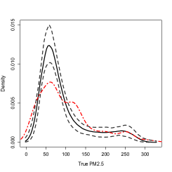
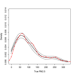
The upper panel in Figure 6 shows the estimated pdfs based on the Bspline MLE and the deconvolution method. Compared with the kernel estimator in the same plots which ignores the measurement errors, the Bspline MLE shows more difference than the deconvolution estimator. In fact, the noise-to-signal ratio is more than , hence measurement error issue is likely not ignorable.
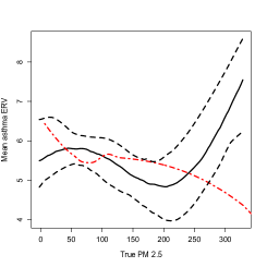
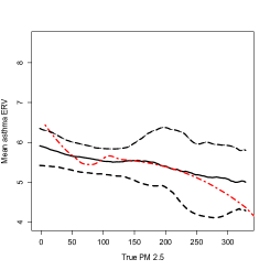
The lower panel in Figure 6 provides the estimated mean of as a function of . The Bspline semiparametric estimator shows a fluctuating pattern in the range from 0 to 200, although the pattern is not significant. In the range of PM2.5 concentration larger than 200 (about 11.3% of the observations), it shows clearly an increasing trend, which agrees with the conclusion in Fan et al. (2016) that the exposure to high PM2.5 has an adverse effect on asthma onset. In contrast, the relation from the deconvolution estimator is similar to that of the local linear regression estimator ignoring the measurement errors, and it is unable to detect the increasing trend of the asthma ERVs as the PM2.5 level increases.
6 Discussion
We have developed a Bspline-assisted MLE for nonparametric pdf estimation and a Bspline-assisted semiparametric estimator for nonparametric regression mean function estimation, in the situation that the covariates are compactly supported and measured with error. The performance of both procedures are superior to the widely used deconvolution methods that do not assume compact support on the covariates, in terms of both their theoretical convergence rate and their numerical performance.
A key difference between our procedures and the deconvolution procedures is that we restrict our interest in estimating the functions on a compact set while the deconvolution method does not impose such an assumption. Practically, the possible range of a random variable is indeed finite, and the relevant information is needed only for functions in a finite range, we consider the compact support assumption to be mild. We are thus very curious if deconvolution methods can achieve the same convergence property in such case, with possibly some modifications on the existing procedures. To this end, Hall & Qiu (2005) provides some relevant results based on a discrete Fourier transform and its inverse, while we leave this general question as an open problem for researchers who specialize in deconvolution methods.
Our method is the first non-deconvolution procedure that achieves the standard nonparametric convergence rate, the same rate as that obtained without measurement error. It would be interesting to investigate if other methods, such as kernel or Fourier series methods, can also attain such rate.
The density and regression function estimation problems studied in this work are the most basic ones. In practice, various complications may occur. For example, the error distribution may not be known and need to be estimated parametrically or nonparametrically based on repeated measurements or other instruments. If one estimates parametrically first then insert it into our procedure, it will not have first order effect. However, if is estimated nonparametrically, it will in general affect both the bias and variance of the resulting estimation of both the density and regression functions. See Delaigle & Hall (2016) for deconvolution based estimation incorporating an unknown error distribution.
Appendix
A.1 Proof of Theorem 1
Recall that, is the subvector of without the first element.
A.2 Proof of Theorem 2
Further, we have
The last equality holds by Proposition 4. Taking expectations on both sides, because the above leading term has mean 0 and is of order , we have
Therefore,
When , we further have
This proves the result. ∎
Acknowledgments
We thank Yang Li for providing the daily asthma emergency room visits data. Ma’s research was partially supported by grants from NSF (1608540) and NIH (HL138306, NS073671). Carroll’s research was supported by a grant from the National Cancer Institute (U01-CA057030).


| pdf estimation: | ||||||
| Bspline MLE | Deconvolution | |||||
| Model II(a) | 0.203 | 0.156 | 0.107 | 0.238 | 0.212 | 0.160 |
| Model II(b) | 0.213 | 0.155 | 0.104 | 0.230 | 0.197 | 0.158 |
| Model II(c) | 0.230 | 0.181 | 0.131 | 0.315 | 0.242 | 0.230 |
| mean estimation: | ||||||
| Bspline semiparametric | Deconvolution | |||||
| Model II(a) | 0.370 | 0.263 | 0.175 | 0.908 | 0.796 | 0.762 |
| Model II(b) | 0.425 | 0.264 | 0.163 | 0.857 | 0.828 | 0.779 |
| Model II(c) | 0.414 | 0.291 | 0.219 | 0.880 | 0.832 | 0.801 |

References
- (1)
- Berry et al. (2002) Berry, S. M., Carroll, R. J. & Ruppert, D. (2002), ‘Bayesian smoothing and regression splines for measurement error problems’, Journal of the American Statistical Association 97, 160–169.
- Carroll & Hall (1988) Carroll, R. J. & Hall, P. (1988), ‘Optimal rates of convergence for deconvolving a density’, Journal of the American Statistical Association 83, 1184–1186.
- Conway (1990) Conway, J. B. (1990), A Course in Functional Analysis, Springer-Verlag, New York.
- De Boor (1978) De Boor, C. (1978), A Practical Guide to Splines, Springer-Verlag, New York.
- Delaigle & Gijbels (2002) Delaigle, A. & Gijbels, I. (2002), ‘Estimation of integrated squared density derivatives from a contaminated sample’, Journal of the Royal Statistical Society: Series B 64, 869–886.
- Delaigle & Hall (2016) Delaigle, A. & Hall, P. (2016), ‘Methodology for non-parametric deconvolution when the error distribution is unknown’, Journal of the Royal Statistical Society: Series B 78, 231–252.
- Fan (1991) Fan, J. (1991), ‘On the optimal rates of convergence for nonparametric deconvolution problems’, Annals of Statistics 19, 1257–1272.
- Fan et al. (2016) Fan, J., Li, S., Fan, C., Bai, Z. & Yang, K. (2016), ‘The impact of pm2.5 on asthma emergency department visits: a systematic review and meta-analysis’, Environmental Science and Pollution Research 23, 843–850.
- Fan & Truong (1993) Fan, J. & Truong, Y. K. (1993), ‘Nonparametric regression with errors in variables’, Annals of Statistics 21, 1900–1925.
- Hall & Qiu (2005) Hall, P. & Qiu, P. (2005), ‘Discrete-transform approach to deconvolution problems’, Biometrika 92, 135–148.
- Liu & Taylor (1989) Liu, M. C. & Taylor, R. L. (1989), ‘A consistent nonparametric density estimator for the deconvolution problem’, Canadian Journal of Statistics 17, 427–438.
- Ma et al. (2015) Ma, S., Carroll, R. J., Liang, H. & Xu, S. (2015), ‘Estimation and inference in generalized additive coefficient models for nonlinear interactions with high-dimensional covariates’, Annals of Statistics 43, 2102–2131.
- Masri & Redner (2005) Masri, R. & Redner, R. A. (2005), ‘Convergence rates for uniform b-spline density estimators on bounded and semi-infinite domains’, Nonparametric Statistics 17, 555–582.
- Mission-China (2016) Mission-China (2016), ‘Accessed:09-30’, http://www.stateair.net/web/historical/1/1.html.
- Sarkar et al. (2014) Sarkar, A., Mallick, B. K. & Carroll, R. J. (2014), ‘Bayesian semiparametric regression in the presence of conditionally heteroscedastic measurement and regression errors’, Biometrics 70(4), 823–834.
- Staudenmayer et al. (2008) Staudenmayer, J., Ruppert, D. & Buonaccorsi, J. P. (2008), ‘Density estimation in the presence of heteroscedastic measurement error’, Journal of the American Statistical Association 103, 726–736.
- Stefanski & Carroll (1990) Stefanski, L. A. & Carroll, R. J. (1990), ‘Deconvoluting kernel density estimators’, Statistics 21, 169–184.
- Tsiatis & Ma (2004) Tsiatis, A. A. & Ma, Y. (2004), ‘Locally efficient semiparametric estimators for functional measurement error models’, Biometrika 91, 835–848.
- Wang & Yang (2009) Wang, L. & Yang, L. (2009), ‘Spline estimation of single-index models’, Statistica Sinica 19(2), 765–783.
- Xu et al. (2016) Xu, Q., Li, X., Wang, S., Wang, C., Huang, F., Gao, Q., Wu, L., Tao, L., Guo, J., Wang, W. et al. (2016), ‘Fine particulate air pollution and hospital emergency room visits for respiratory disease in urban areas in beijing, china, in 2013’, PloS One 11, e0153099.
- Zhang (1990) Zhang, C. H. (1990), ‘Fourier methods for estimating mixing densities and distributions’, Annals of Statistics 18, 806–830.