Calibration of Sobol indices estimates in case of noisy output
Abstract
This paper presents a simple noise correction method for Sobol’ indices estimation. Sobol’ indices, especially total Sobol’ indices are quite sensitive to the noise in the output and tend to be severly biased (overestimated) if no noise correction is done, which may make their computation meaningless in case of even quite moderate noise levels. Proposed method allows to get approximately unbiased noise free estimation of Sobol’ indices at the cost of variance of estimate increase if noise can be represented as a combination of additive and multiplicative stationary noise. Proposed method is more straightforward than schemes found in the literature and does not introduce any assumptions on the function and noise distribution (except that it assumes noise to be stationary and be a combination of additive and multiplicative). One of the appealing features is that there is actual analytical noise correction expression derived.
1 Introduction
Computational models became really important in lots of different areas ([1], [2], [3]). Often they are so complex that special tools are needed to analyse their behavior. Sensitivity analysis is the study of how the variations in the output of a mathematical model or system can be apportioned to different variations in its inputs.
Sensitivity analysis includes a wide range of metrics and techniques. Most notable are the Morris method [13], linear regression-based methods [4], variance-based methods [6]. Among others, Sobol’ (sensitivity) indices are a common metric to evaluate the influence of model parameters [5]. Sobol’ indices describe the portion of the output variance explained by different input parameters and combinations thereof. This method is especially useful for the case of nonlinear computational models [7].
Different approaches are applied to estimate Sobol indices. In [8] A. Saltelli uses the Fourier amplitude sensitivity test (FAST) algorithm, which requires to generate complex deisgn of experiment, but is considered to be the most accurate approach. In [10] E. Plischke proposed an EASI algorithm, that allows to efficiently compute Sobol indices on any given sample. In [9] G. Glen demonstrates correlation based method with the correction to the spurious correlation, which is very convenient to compute confidence intervals for the indices and for handling Not-a-number-values in the design.
Generally when starting an analysis two types of Sobol indices are computed:
-
1.
Main indices () which take into account only sole influence of each feature while all others being fixed. These indexes tell what portion of output variance would be described by considered input provided all other inputs are fixed at their mean values.
-
2.
Total indices () which take into account interactions between features. These indexes tell what portion of output variance would be lost if we fix considered feature to its mean value, while still vary others.
It’s important that all Sobol’ indices estimates are very sensitive to the noise in the output (or some uncontrollable input parameters that change arbitrary on different function calls). Having even moderate noise leads to significant overestimation of main and especially total indices making analysis futile, provided no noise correction is done.
When doing the sensitivity analysis expert usually knows if his function is noisy beforehand, so it makes sense to have special estimation procedure in the setting with noisy output.
In [22] here is a review of Probabilistic Sensitivity Analysis (PSA) — study the impact of uncertainties in design variables and noise parameters on the probabilistic characteristics of a design performance. There were some attempts in the literature aimed to introduce noise correction to the Sobol indices estimation. In [18] authors tried to directly estimate influence of noise and focuses on models that depend on scalar parameter vector X and involve some stochastic process simulations or random fields as input parameters, where can be spatial coordinates, time scale or any other physical parameters. Fort and others ([21]) consider is a separable Hilbert space endowed with the scalar product and a linear regression model , where for , — independent centered, -valued, stochastic processes, , are elements of , and is a centered noise independent of the processes . They construct natural estimators of the Sobol indices for whom they prove asymptotic normality and efficiency, using Karhunen-Loeve decomposition of the processes . Lewandowski ([23]) explored correlation ratio, estimate of sensivity, based on Sobol indices, and applied it to model , where is the explaining variable and is added noise. Interesting results on approximation for features of ANOVA-decomposition components are presented in [24]. In this work authors consider ANOVA-decomposition (base for Sobol indices theory) and model of function with additive noise. One more work with same theme — [25]. Function model with additive noise is considered in works on sensitivity analysis not for only Sobol indices, for example, see [26].
In this article we propose simple and straightforward method to remove noise induced distortion from Sobol’ indices estimates. The idea of the method is to introduce virtual input for which we know function does not really depend on and variations of the output one obervers when one changing this input are only due to noise.
Such trick allows one to derive analytical noise correction formulas for main and total Sobol’ indices. Such approach works in case noise in the data is stationary and is a combination of additive and multiplicativ components. Also we show that if noise has more complex structure no precise noise correction procedure can be done.
The advantages of proposed approach are:
-
1.
It is very simple and straightforward to apply.
-
2.
It does not depend on estimation approach, so expert can still select the one suitable for the task.
-
3.
It does not introduce additional source of error (unlike meta models, which often bring to the analysis additional distortions).
The paper is organised as follows:
2 Sensitivity Indices
Definition 1
Let us define a computational model , where
is a vector of input variables (or parameters or features),
is an output variable and is a design space. The model describes the behavior of some physical system of interest.
Note that in the definition above one may consider noise as just one of the inputs whose value is not controlled by experimenter, is unknown and changes arbitrary. So it is possible to introduce noise in the framework without adding complexity to expressions.
Assuming that the function is square-integrable with respect to distribution (i.e. ), we have the following unique Sobol’ decomposition of (see [5]) given by
which satisfies:
where and are index sets: .
Due to orthogonality of the summands, we can decompose the variance of the model output:
In this expression is the contribution of summand to the output variance.
Definition 2
The sensitivity index (Sobol’ index) of variable set is defined as
The sensitivity index describes the amount of the total variance explained by the variance in the subset of model input variables .
Definition 3
Main () and total () Sobol’ indices are defined as
3 Noise correction formula
Definition 4
Let us consider the following working model of noisy output:
where and are some random noise, is some virtual variable generating noise (i.e. seed of random generator),
Definition 5
Let us denote (i.e. set of all features except -th).
Definition 6
Let and be mean and total Sobol’ indices computed for function (i.e. with noise in present).
Definition 7
Let and be mean and total Sobol’ indices computed for function (i.e. with noise removed).
Having defined necessary concepts we can state the noise correction procedure proposed in the paper.
Statement 1
If dependency has same structure as in Definition 4 and and do not depend on . Then it holds that:
| (1) |
| (2) |
Proof 1
Let us calculate Sobol indices for function :
Besides, we can consider :
Then
From that one can easily derive and .
Note that results presented above can be used with any indices estimation schema and noise distribution. The only requirement is the stationariness of noise.
Also note that to compute noise corrected Sobol’ indices one should use several estimates of noised indices. Which would lead no increased variance of final estimate.
Statement 2
If the used Sobol’ indices estimation procedure for estimation of , , is unbiased and estimation errors of , , are uncorrelated, then estimates of , from equations (1) and (2) the bias (first order correction) of estimators:
| (3) |
| (4) |
And corresponding variances are:
| (5) |
| (6) |
Proof 2
Looking at equations (5) and (6) one may see that due to a denominator the greater noise level is the greater the variance of noise corrected estimator would be. This effect is accordance with experimental results presented in Section 4.
If method from [9] is used to compute Sobol’ indices can be computed via bootstrap and corresponding corrections to the , estimates could be made.
4 Experiments
In this section we demonstrate how our approach performs on number of examples.
We will use method from [9] with implementation taken from library [11] (library version 6.3 was used).
4.1 Example 1: Linear function
At first let us consider linear function
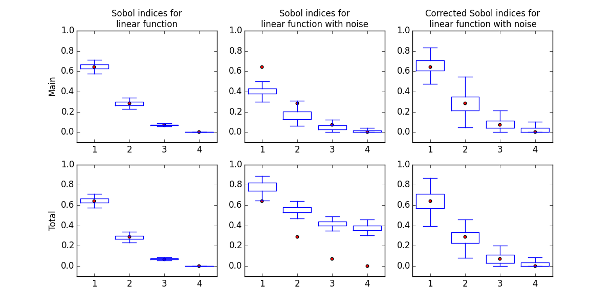
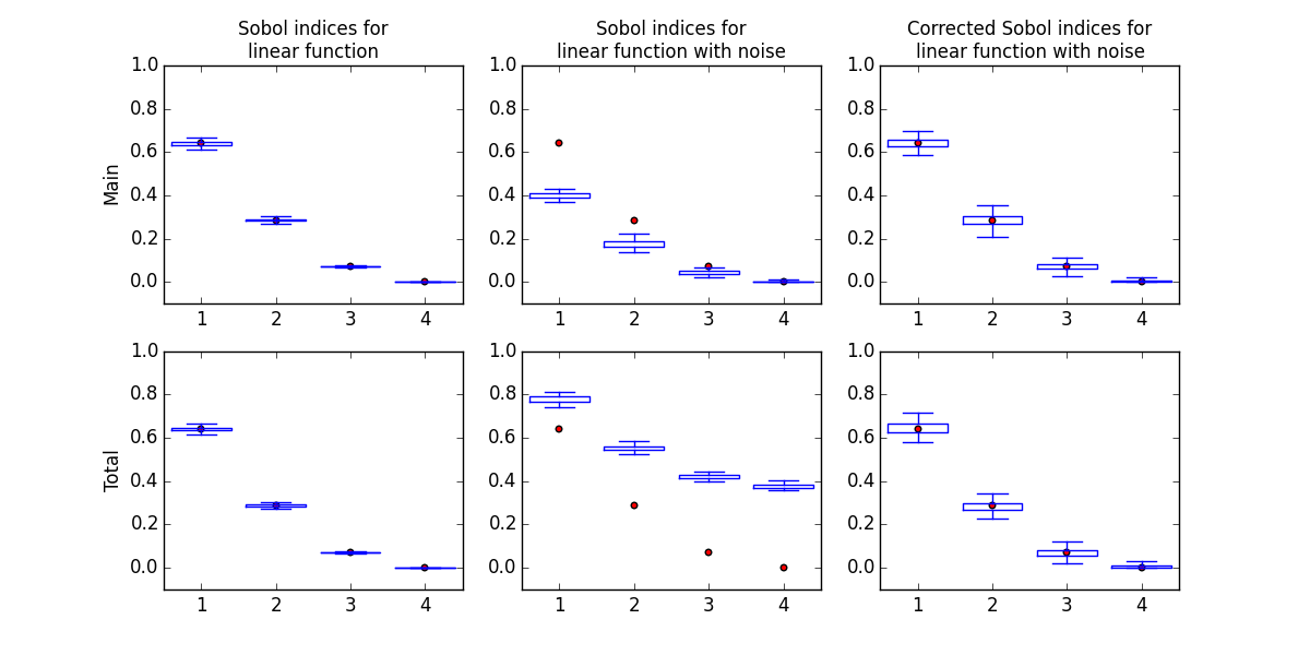
True values of Sobol indices are equal to for both main and total indices as no interactions are present.
We set noise parameters to be .
Plots showing estimation results for main and total indices are shown on figures 1 and 2. Left column shows performance of estimator if no noise were present, middle column shows estimation results for noisy function if no noise correction was done, right column shows results of noise corrected estimator. Red dots show true values of indices if noise removed.
4.2 Example 2: Sobol’ function
Another common function to consider in papers about Sobol’ indices is Sobol’ function (it’s properties was studied in [5]).
where .
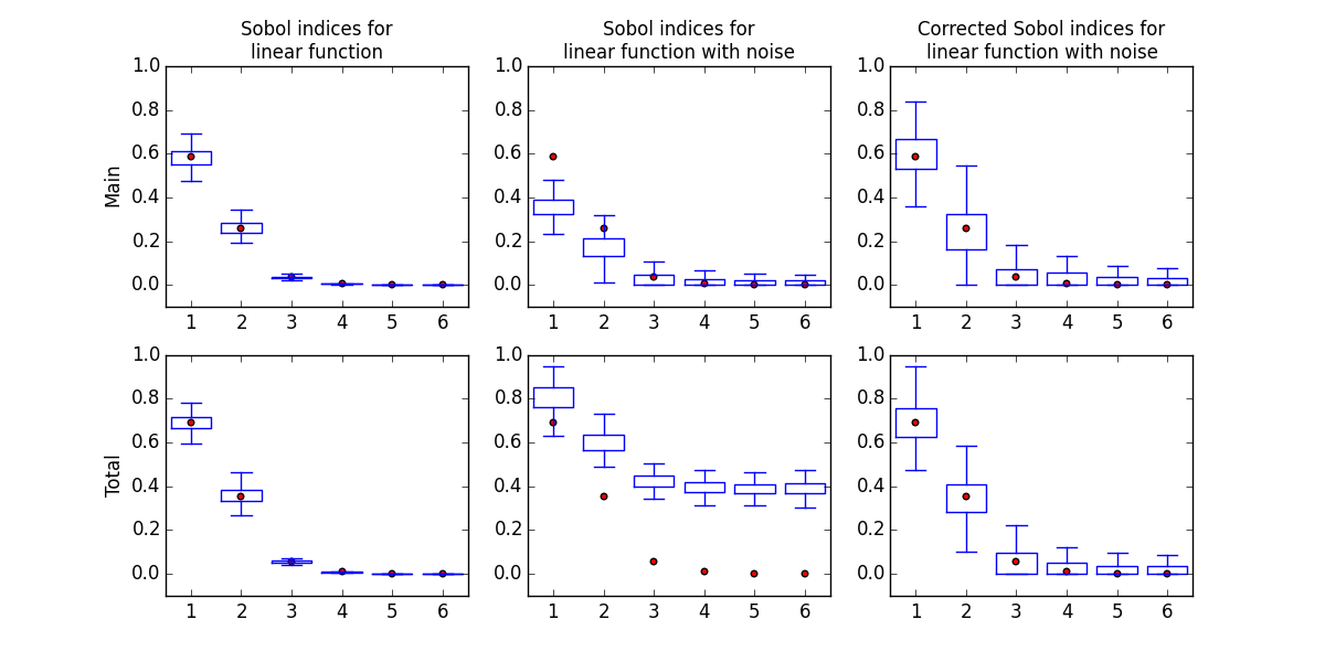
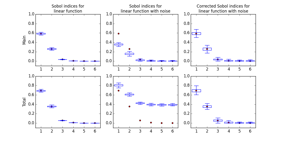
It’s main indices are approximately equal to , , , , , and total indices are , , , , , .
We set noise parameters to be .
Plots showing estimation results for main and total indices are shown on figures 3 and 4. Left column shows performance of estimator if no noise were present, middle column shows estimation results for noisy function if no noise correction was done, right column shows results of noise corrected estimator.
For both examples one may see that corrected estimates have much lower bias, but increased variance, which however decreases as sample size gets bigger.
4.3 Example 3: Steel column under stress.
Let us consider a bit more complex example – model a steel column under stress. This function is used to demonstrate uncertainty quantification, for example, in works [19], [20]. The dependency can be written as following formlua:
where
The steel column stress depends on 9 different parameters, see table LABEL:tab1.
| Parameter | Distribution | Meaning | Measure |
|---|---|---|---|
| dead weight load | N | ||
| variable load | N | ||
| variable load | N | ||
| flange breadth | mm | ||
| flange thickness | mm | ||
| profile height | mm | ||
| initial deflection | mm | ||
| Young’s modulus | MPa |
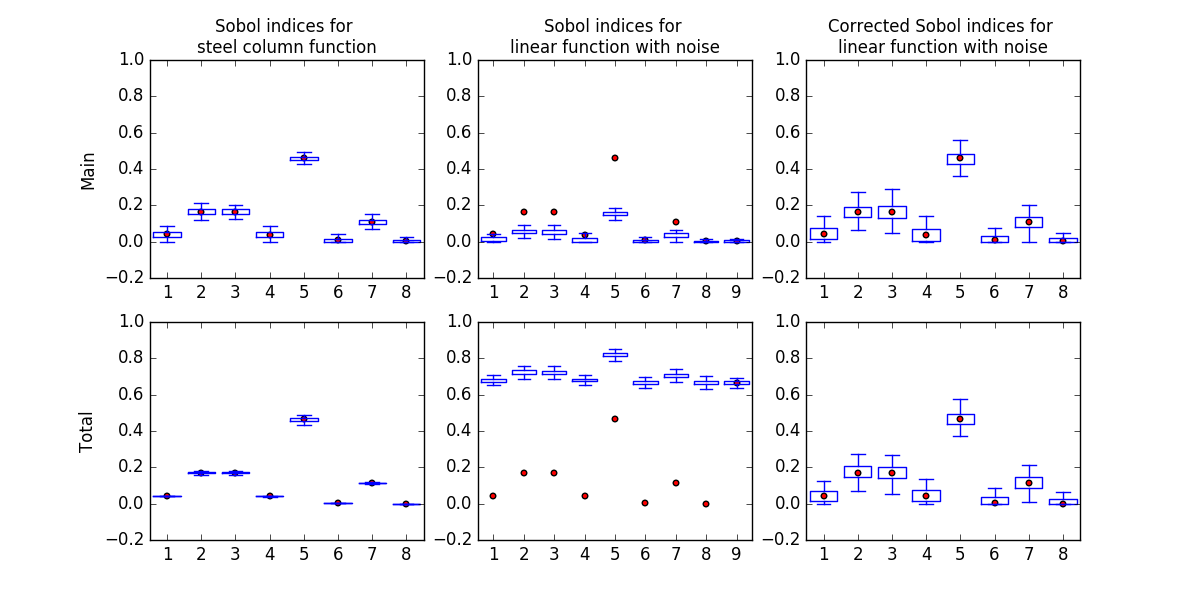
In the experiment we introduce noise to the model by assuming that we can not control variable. Firstly, we estimate Sobol indices, using and will consider them as true values in the analysis..
Then we add fictive variable and set random values to on each evaluation (with distribution ).
Obtained estimates of Sobol indices are given below. First column show estimates of function without noise, second — estimates of function with noise (and sobol indices for fictive variable too), and third — corrected estimates of function with noise.
5 Conclusion
We presented a noise correction method for Sobol’ indices computation and demonstrated it’s performance on several toy examples. We think the method is easier to use and, because of its simplicity, more reliable than existing alternatives when one needs to perform sensitivity analysis on the noisy functions (which often happens with numeric solvers where noise may be introduced due to convergence issues).
Method can be applied on top of any Sobol’ indices estimatior and usage of explicit formulas to do noise correction allows for straightforward errors propagation in case confidence intervals of original Sobol’ indices estimator can be computed.
Main current limitation of the method is its imposed assumption on the noise structure, which in some cases may be not possible to easily check a priory. Though we hope that we will be able to consider more general setting in the future.
One particular possible way to loosen the requirements of noise may be through analysis of higher order indices which method from [9] allows to do without additional computational budget.
Also it was observed above that noise correction procedure tends to increase variance of corrected indices estimates. Due to that it may make sense to use additional variance reduction techniques in base estimation procedures. One of the promising approaches may be in using of special designs of experiments that reduce the variance of estimation [28].
6 Acknowledgements
The research of the first author was conducted in IITP RAS and supportedsolely by the Russian Science Foundation grant (project 14-50-00150).
References
- [1] K.J.Beven. Rainfall-Runoff Modelling-The Primer, Wiley,360 pp, Chichester,2000.
- [2] P. Dayan and L. F. Abbott (2001). Theoretical Neuroscience: Computational and Mathematical Modeling of Neural Systems (MIT Press, Cambridge, MA).
- [3] S. Grihon, E.V. Burnaev, M.G. Belyaev, and P.V. Prikhodko. Surrogate Modeling of Stability Constraints for Optimization of Composite Structures. Surrogate-Based Modeling and Optimization. Engineering applications. Eds. by S. Koziel, L. Leifsson. Springer, 2013. P. 359-391.
- [4] B. Iooss, P. Lemaitre. A review on global sensitivity analysis methods. In: Meloni C, Dellino G (eds) Uncertainty management in Simulation-Optimization of Complex Systems: Algorithms and Applications, Springer, 2015.
- [5] I. M. Sobol’. Sensitivity estimates for nonlinear mathematical models. Math. Model. Comp. Exp. 1, 407–414, 1993.
- [6] A. Saltelli. Global Sensitivity Analysis The Primer. Wiley, 2008.
- [7] A. Saltelli, P. Annoni. How to avoid a perfunctory sensitivity analysis. Environ. Modell. Softw. 25, 1508-1517, 2010
- [8] A. Saltelli. A quantitative model-independent method for global sensitivity analysis of model output. Technometrics, 41:39–56, 1999.
- [9] G. Glen. Estimating Sobol sensitivity indices using correlations. Environmental Modelling and Software, volume 37, pages 157–166, 2012
- [10] E. Plischke. An Effective Algorithm for Computing Global Sensitivity Indices (EASI), 2010.
- [11] https://www.datadvance.net/product/macros/manual/6.4/guide/gtsda/sensitivity.html
- [12] A. Degasperi and S. Gilmore. Sensitivity Analysis of Stochastic Models of Bistable Biochemical Reactions. Formal Methods for Computational Systems Biology. Volume 5016 of the series Lecture Notes in Computer Science pp 1-20
- [13] Max D. Morris. Factorial Sampling Plans for Preliminary Computational Experiments. Technometrics, Vol. 33, No. 2, pp. 161-174, May, 1991
- [14] I.M. Sobol. Sensivity Estimates for Nonlinear Mathematical Models. Mathematical Modeling and Computational Experiment. NY, 1993.
- [15] J. L. Hart, A. Alexanderian, P. A. Gremaud. Efficient computation of Sobol’ indices for stochastic models.
- [16] E. Plischke, E. Borgonovo, C. L. Smith. Global sensitivity measures from given data, 2013.
- [17] T. A. Mara, S. Tarantola. Variance-based sensitivity indices for models with dependent inputs. Reliability Engineering and System Safety, 2012.
- [18] B. Iooss, M. Ribatet and A. Marrel. Global sensitivity analysis of stochastic computer models with generalized additive models.
- [19] M. S. Eldred, C. G. Webster, P. Constantine. Evaluation of non-intrusive approaches for Wiener-Askey generalized polynomial chaos. In Proceedings of the 10th AIAA Non-Deterministic Approaches Conference, number AIAA-2008-1892, Schaumburg, IL, vol. 117, p. 189, April, 2008.
- [20] N. Kuschel, R. Rackwitz. Two basic problems in reliability-based structural optimization. Mathematical Methods of Operations Research, 46(3), 309-333, 1997.
- [21] J.-C. Fort, T. Klein, A. Lagnoux, B. Laurent. Estimation of the Sobol indices in a linear functional multidimensional model. Journal of Statistical Planning and Inference, Elsevier, 2013, 143 (9), pp.1590-1605.
- [22] H. Liu, W. Chen. Probabilistic Sensitivity Analysis Methods for Design under Uncertainty. 10th AIAA/ISSMO Multidisciplinary Analysis and Optimization Conference.
- [23] D. Lewandowski, R. M. Cooke, R. J. D. Tebbens. Sample–based Estimation of Correlation Ratio with Polynomial Approximation. ACM Transactions on Modeling and Computer Simulation (TOMACS), Volume 18 Issue 1, December 2007, Article No. 3.
- [24] X. Wang, Y. Tang, Y. Zhang. Orthogonal arrays for estimating global sensitivity indices of non-parametric models based on ANOVA high-dimensional model representation. Journal of Statistical Planning and Inference, 142 (2012), 1801–1810.
- [25] R. Jin, W. Chen, A. Sudjianto. Analytical Metamodel-Based Global Sensitivity Analysis and Uncertainty Propagation for Robust Design. SAE Technical Paper, 2004-01-0429, 2004.
- [26] O. Roustant, D. Ginsbourger, Y. Deville. DiceKriging, DiceOptim: Two R packages for the analysis of computer experiments by kriging-based metamodeling and optimization. 2012.
- [27] A.J. Scott, C.F.J. Wu. On the asymptotic distribution of ratio and regression estimators. JASA 76: 98–102, 1981.
- [28] E. Burnaev, I. Panin, B. Sudret, Effective design for sobol indices estimation based on polynomial chaos expansions, in: A. Gammerman, Z. Luo, J. Vega, V. Vovk (Eds.), 5th International Symposium, COPA 2016 Madrid, Spain, April 2022, 2016, Proceedings, volume 9653 of Lecture Notes in Artificial Intelligence, Springer International Publishing, 2016, pp. 165–184.