Graph-Based Deep Modeling and Real Time Forecasting of Sparse Spatio-Temporal Data

Abstract.

We present a generic framework for spatio-temporal (ST) data modeling, analysis, and forecasting, with a special focus on data that is sparse in both space and time. Our multi-scaled framework is a seamless coupling of two major components: a self-exciting point process that models the macroscale statistical behaviors of the ST data and a graph structured recurrent neural network (GSRNN) to discover the microscale patterns of the ST data on the inferred graph. This novel deep neural network (DNN) incorporates the real time interactions of the graph nodes to enable more accurate real time forecasting. The effectiveness of our method is demonstrated on both crime and traffic forecasting.

1. Introduction

Accurate spatio-temporal (ST) data forecasting is one of the central tasks for artificial intelligence with many practical applications. For instance, accurate crime forecasting can be used to prevent criminal behavior, and forecasting traffic is of great importance for urban transportation system. Forecasting the ST distribution effectively is quite challenging, especially at hourly or even finer temporal scales in micro-geographic regions. The task becomes even harder when the data is spatially and/or temporally sparse. There are many recent efforts devoted to quantitative study of ST data, both from the perspective of statistical modeling of macro-scale properties and deep learning based approximation of micro-scale phenomena. We briefly mention a few relevant works. Mohler et al pioneered the use of the Hawkes process (HP) to predict crime. Recent field trials (Mohler:2011JASA, ) show these models can outperform crime analysts, and are now used in commercial software deployed in over 50 municipalities worldwide. In (Kang:2017Crime, ), the authors utilized a convolutional neural network (CNN) to extract the features from the historical crime data, and then used a support vector machine (SVM) to classify whether there will be crime or not at the next time slot. Zhang et al (Junbo:2017, ) create an ensemble of residual networks (He:2016ResNet, ), named ST-ResNet, to study and predict traffic flow. Additional applications include (Jain:2016, ) who use the ST graph to represent human environment interaction, and proposed a structured recurrent neural network (RNN) for semantic analysis and motion reasoning. The combination of video frame-wise forecasting and optical flow interpolation allows for the forecasting of the dynamical process of the robotics motion (Holden:2017, ). RNNs have also been combined with point processes to study taxi and other data (Du:2016, ).

This paper builds on our previous work (BaoWang:2017DL1, ) in which we applied ST-ResNet, along with data augmentation techniques, to forecast crime on a small spatial scale in real time. We further showed that the ST-ResNet can be quantized for crime forecasting with only a negligible precision reduction (BaoWang:2017DL2, ). Moreover, ST data forecasting also has wide applications in computer vision (LeCun:2015Nature, ; Hochreiter:1997NC, ; Jain:2016, ; Holden:2017, ; Li:2016GatedGraphNN, ). Many previous CNN-based approaches for ST forecasting map the spatial distribution to a rectangular box partitioned with a rectangular grid. The data at a certain timescale is represented by a histogram on the grid. Finally, a CNN is used to predict the future histogram. This prototype is sub-optimal from two aspects. First, the geometry of a city is usually highly irregular, resulting in the city’s configuration taking up only a small portion of its bounding box. This introduces unnecessary redundancy into the algorithm. Second, the spatial sparsity can be exacerbated by the spatial grid structure. Directly applying a CNN to fit the extreme sparse data will lead to all zero weights due to the weight sharing of CNNs (BaoWang:2017DL2, ). This can be alleviated by using spatial super-resolution(BaoWang:2017DL2, ), with increased computational cost. Moreover this lattice based data representation omits geographical information and spatial correlation within the data itself.

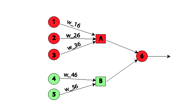
In this work, we develop a generic framework to model sparse and unstructured ST data. Compared to previous ad-hoc spatial partitioning, we introduce an ST weighted graph (STWG) to represent the data, which automatically solves the issue caused by spatial sparsity. This STWG carries the spatial cohesion and temporal evolution of the data in different spatial regions over time. We infer the STWG by solving a statistical inference problem. For crime forecasting, we associate each graph node with a time series of crime intensity in a zip code region, where each zip code is a node of the graph. As is shown in (Mohler:2011JASA, ), the crime occurrence can be modeled by a multivariate Hawkes process (MHP), where the self and mutual-exciting rates determines the connectivity and weights of the STWG. To reduce the complexity of the model, we enforce the graph connectivity to be sparse. To this end, we add an additional $L_{1}$ regularizer to the maximal likelihood function of MHP. The inferred STWG incorporates the macroscale evolution of the crime time series over space and time, and is much more flexible than the lattice representation. To perform micro-scale forecasting of the ST data, we build a scalable graph structured RNN (GSRNN) on the inferred graph based on the structural-RNN (SRNN) architecture (Jain:2016, ). Our DNN is built by arranging RNNs in a feed-forward manner: We first assign a cascaded long short-term memory (LSTM) (we will explain this in the following paragraph) to fit the time series on each node of the graph. Simultaneously, we associate each edge of the graph with a cascaded LSTM that receives the output from neighboring nodes along with the weights learned from the Hawkes process. Then we feed the tensors learned by these edge LSTMs to their terminal nodes. This arrangement of edge and node LSTMs gives a native feed-forward structure that is different from the classical multilayer perceptron. A neuron is the basic building block of the latter, while our GSRNN is built with LSTMs as basic units. The STWG representation together with the feed-forward arranged LSTMs build the framework for ST data forecasting. The flowchart of our framework is shown in Fig. 1.

Figure 1. Flow chart of the algorithm.

Our contribution is summarized as follows:

• We employ a compact STWG to represent the ST sparse unstructured data, which automatically encodes important statistical properties of the data.

• We propose a simple data augmentation scheme to allow DNN to approximate the temporally sparse data.

• We generalize the SRNN(Jain:2016, ) to be bi-directional, and apply a weighted average pooling which is more suitable for ST data forecasting.

• We achieve remarkable performance on real time crime and traffic forecasting at a fine-grained scale.

In section 2, we describe the datasets used in this work, including data acquisition, preprocessing, spectral and simple statistical analysis. In section 3, we present the pipeline for general ST data forecasting, which contains STWG inference, DNN approximation of the historical signals, and a data augmentation scheme. Numerical experiments on the crime and traffic forecasting tasks are demonstrated in sections 4 and 5, respectively. The concluding remarks and future directions are discussed in section 6.

2. Dataset Description and Simple Analysis

We study two different datasets: the crime and traffic data. The former is more irregular in space and time, and hence is much more challenging to study. In this section we describe these datasets and introduce some preliminary analyses.

2.1. Crime Dataset

2.1.1. Data Collection and Preprocessing

We consider crime data in Chicago (CHI) and Los Angeles (LA). In our framework, historical crime and weather data are the key ingredients. Holiday information, which is easy to obtain, is also included. The time intervals studied are 1/1/2015-12/31/2015 for CHI and 1/1/2014-12/31/2015 for LA, with a time resolution of one hour. Here we provide a brief description of the acquisition of these two critical datasets.

Weather Data

We collect the weather data from the Weather Underground data base through a simple web crawler. We select temperature, wind speed, and special events, including fog, snow, rain, thunderstorm for our weather features. All data is co-registered in time to the hour.

Crime Data

The CHI crime data is downloaded from the City of Chicago open data portal. The LA data is provided by the LA Police Department (LAPD). Compared to CHI data, the LA crime data is sparser and more irregular in space. We first map the crime data to the corresponding postal code using QGIS software (QGIS_software, ). A few crimes in CHI (less than $0.02\%$) cannot be mapped to the correct postal code region, and we simply discard these events. For the sake of simplicity, we only consider zip code regions with more than 1000 crime events over the full time period. This filtering criterion retains over 95 percent of crimes for both cities, leaving us with 96 postal code regions in LA and 50 regions in CHI.

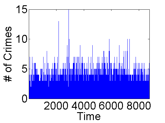
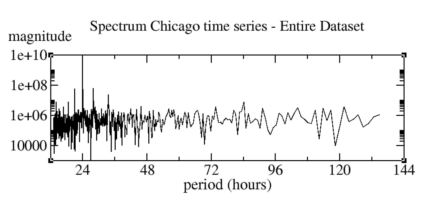
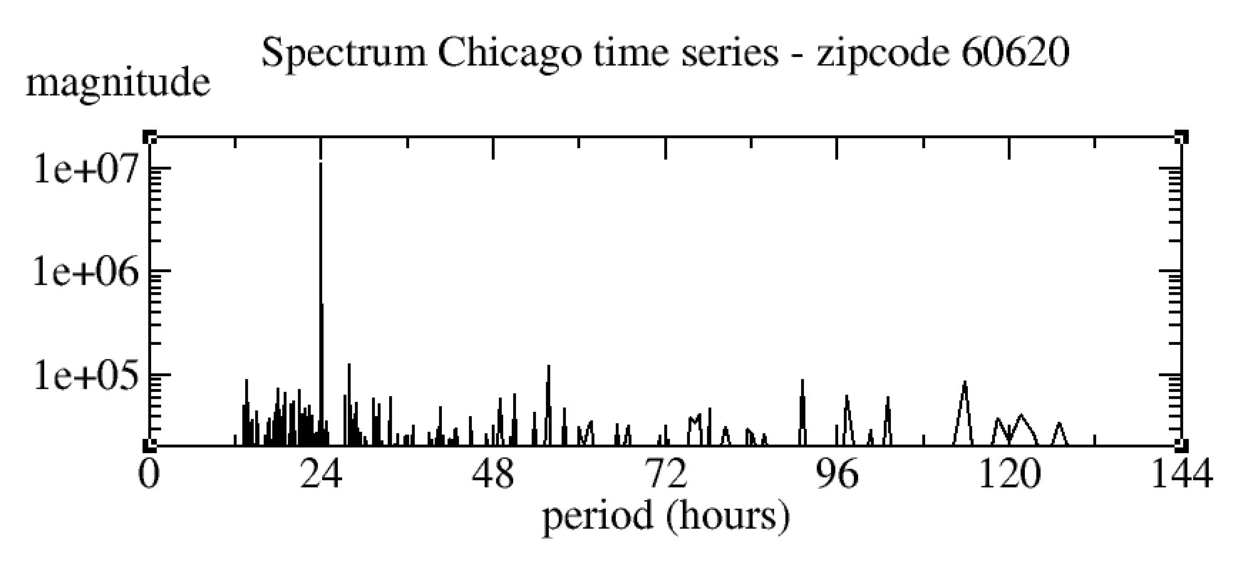
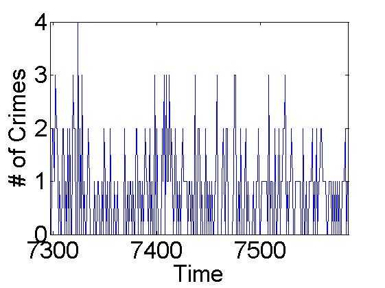
2.1.2. Spectrum of the Crime Time Series

Figure 2 plots the hourly crime intensities over the entire CHI and a randomly selected zip code region. Though the time series are quite noisy, the spectrum exhibits clear diurnal periodicity as shown in Fig. 3.

Figure 2. Example plots of the hourly crime intensities for the entire 2015 CHI (left) and the 2015 60620 zip code (right).

Figure 3. Spectrum of the time series from Fig. 2.

2.1.3. Statistical Analysis of Crime Data

Evidence suggests that crime is self-exciting (RN3516, ), which is reflected in the fact that crime events are clustered in time. The arrival of crimes can be modeled as a Hawkes process (HP) (Mohler:2011JASA, ) with a general form of conditional intensity function:

(1) $$\lambda(t)=\mu+a\sum_{t_{i}\leq t}g(t-t_{i})$$

where $\lambda(t)$ is the intensity of events arrival at time $t$, $\mu$ is the endogenous or background intensity, which is simply modeled by a constant, $a$ is the self-exciting rate, and $g(t)$ is a kernel triggering function. In (Zipkin:2016, ), it found that an exponential kernel, i.e., $g(t)=w\exp(-wt)$ where $\frac{1}{w}$ models the average duration of the influence of an event, is a good description of crime self-excitation. To calibrate the HP, we use the expectation-maximisation (EM) algorithm (Veen:2008, ). Simulation of the HP is done via a simple thinning algorithm (Laub:2015, ).

The HP fits to the crime time series in zip code region 60620 yields $\lambda(t)=0.7562+\sum_{t_{i}<t}0.4673*31.6301*\exp(-31.6301*(t-t_{i}))$, which shows that on average, each crime will have 0.4673 offspring. Furthermore, we noticed that the duration of the influence is roughly a constant over different zip code regions.

(a) Exact	(b) one path sampled	(c) ensemble 5000

Figure 4. Exact and simulated hourly crime intensities for CHI 60620 in the first two weeks of Nov 2015. (a), (b), and (c) depict the exact, one path sampled from the HP, and the ensemble average of 5000 paths, respectively.

Figure 4 shows the exact and simulated crime intensities in the first two weeks in Nov 2015 over zip code region 60620. Both the exact and simulated time series demonstrate clustered behavior, which confirms the assumption that crime time series is self-exciting, and supports the contention that the HP is a suitable model. However, the simulate intensity peaks are shifted relative to the exact ones. If we use the HP to do the crime forecasting, we typically do an ensemble average of many independent realizations of the HP, as is shown in panel (c). However, this ensemble average differs hugely from the exact crime time series. To capture fine scale patterns we will use DNN.

2.2. Traffic Data

We also study the ST distribution of traffic data (Junbo:2017, ). The data contains two parts: taxi records from Beijing (TaxiBJ) and bicycle data from New York city (BikeNYC). Basic analyse in (Junbo:2017, ) shows periodicity, meteorological dependence, and other basic properties of these two datasets. The time span for TaxiBJ and BikeNYC are selected time slots from 7/1/2013 to 4/10/2016 and the entire span 4/1/2014-9/30/2014, respectively. The time intervals are 30 minutes and one hour, respectively. Both data are represented in Eulerian representations with lattice sizes to be 32$\times$32 and 16$\times$8, respectively. Traffic flow prediction using this traffic dataset will be selected as benchmark to evaluate our model.

3. Algorithms and Models

Our model contains two components. The first part is a graph representation for the spatio-temporal evolution of the data, where the nodes of the graph are selected to contain sufficient predictable signals, and the topological structure of the graph is inferred from self-exciting point process model. The second component is a DNN to approximate the temporal evolution of the data, which has good generalizability. The advantages of a graph representation are two-fold: on the one hand, it captures the irregularity of the spatial domain; on the other hand, it can capture versatile spatial partitioning which enables forecasting at different spatial scales. In this section, we will present the algorithms for modeling and forecasting the ST sparse unstructured data. The overall pipeline includes: STWG inference, data augmentation, and the structure and algorithm to train the DNN.

3.1. STWG Representation for the ST Data

The entire city is partitioned into small pieces with each piece representing one zip code region, or other small region. This partitioning retains geographical cohesion. In the STWG, we associate each geographic region with one node of the graph. The inference of the graph topological structure is done by solving the maximal likelihood problem of the MHP. We model the time series on the graph by the following MHP $\{N_{t}^{u}|u=1,2,\cdots,U\}$ with conditional intensity functions:

(2) $$\lambda_{u}(t)=\mu_{u}+\sum_{i:t_{i}<t}a_{uu_{i}}g(t-t_{i}),$$

where $\mu_{u}\geq 0$ is the background intensity of the process for the $u$-th node and $t_{i}$ is the time at which the event occurred on node $u_{i}$ prior to time $t$. The kernel is exponential, i.e., $g(t)=w*\exp(-w*t)$.

We calibrate the model in Eq.(2) using historical data. Let $\boldmath{\mu}=(\mu_{u}|u=1,2,\cdots,U)$ and $A=(a_{uu^{\prime}}|u,u^{\prime}=1,2,\cdots,U)$. Suppose we have $m$ i.i.d samples $\{c_{1},c_{2},\cdots,c_{m}\}$ from the MHP; each is a sequence of events observed during a time period $[0,T_{c}]$. The events form a set of pairs $(t_{i}^{c},u_{i}^{c})$ denoting the time $t_{i}^{c}$ and the node $u_{i}^{c}$-th for each event. The log-likelihood of the model is:

(3) $$\mathcal{L}(\mu,A)=\sum_{c}\left(\sum_{i=1}^{n_{c}}\log\lambda_{u_{i}}(t_{i}^{c})-\sum_{u=1}^{U}\int_{0}^{T_{c}}\lambda_{u}(t)dt\right).$$

Similar to the work by Zhou et al (Zha:2013, ), to ensure the graph is sparsely connected, we add an $L_{1}$ penalty, $\lambda|A|_{1}=\lambda\sum_{uu^{\prime}}|a_{uu^{\prime}}|$, to the log-likelihood $\mathcal{L}$ in Eq.(3): $\mathcal{L}_{\lambda}(\mu,A)=-\mathcal{L}+\lambda|A|_{1}$. To infer the graph structure, we solve the optimization problem:

$${\rm argmin}_{\boldmath{\mu},A}\mathcal{L}_{\lambda}(\boldmath{\mu},A),\\ \quad\mbox{s.t.}\ \boldmath{\mu}\geq 0,\ {\rm and}\ \ A\geq 0,$$

where $\boldmath{\mu}\geq 0$ and $A\geq 0$, both are defined element-wise. We solve the above constraint optimization problem by the EM algorithm. The $L_{1}$ constraint is solved by a split-Bregman liked algorithm (Goldstein:2009, ). For a fixed parameter $w$, we iterate between the following two steps until convergence is reached:

• E-Step: Compute the exogenous or endogenous probability:

  $$p_{ii}^{c}=\frac{\mu_{u_{i}^{c}}^{(k)}}{\mu_{u_{i}^{c}}^{(k)}+\sum_{j=1}^{i-1}a_{u_{i}u_{j}}^{(k)}g(t_{i}^{c}-t_{j}^{c})},$$

  $$p_{ij}^{c}=\frac{a_{u_{i}u_{j}}^{(k)}g(t_{i}^{c}-t_{j}^{c})}{\mu_{u_{i}^{c}}^{(k)}+\sum_{j=1}^{i-1}a_{u_{i}u_{j}}^{(k)}g(t_{i}^{c}-t_{j}^{c})}$$

• M-Step: Update parameters:

  $$\mu_{u}^{(k+1)}=\frac{1}{\sum_{c}T_{c}}\left(\sum_{c}\sum_{i=1,u_{i}^{c}=u}^{n_{c}}p_{ii}^{c}\right)$$

  $$a_{uu^{\prime}}^{(k+1)}=\left(\frac{a_{uu^{\prime}}^{(k)}\sum_{c}\sum_{i:u_{i}^{c}=u}\sum_{j<i,u_{j}^{c}=u^{\prime}}p_{ij}^{c}}{\sum_{c}\sum_{j:u_{j}^{c}=u^{\prime}}\int_{0}^{T_{c}-t_{j}^{c}}g(t)dt}\right)^{1/2}$$

  $$a_{uu^{\prime}}^{(k+1)}={\rm shrink}_{\lambda}(a_{uu^{\prime}}^{(k+1)}).$$

The above EM algorithm is of quadratic scaling, which is infeasible for our datasets. To reduce the algorithm’s complexity, instead of considering all events before a given time slot, we do a simple truncation in the E-step based on the localization of the exponential kernel. This truncation simplifies the algorithm from quadratic scaling to almost linear scaling. In the inference of the STWG, we set the hyper-parameter $\lambda$ to be $0.01$.

3.1.1. Results on STWG Inference

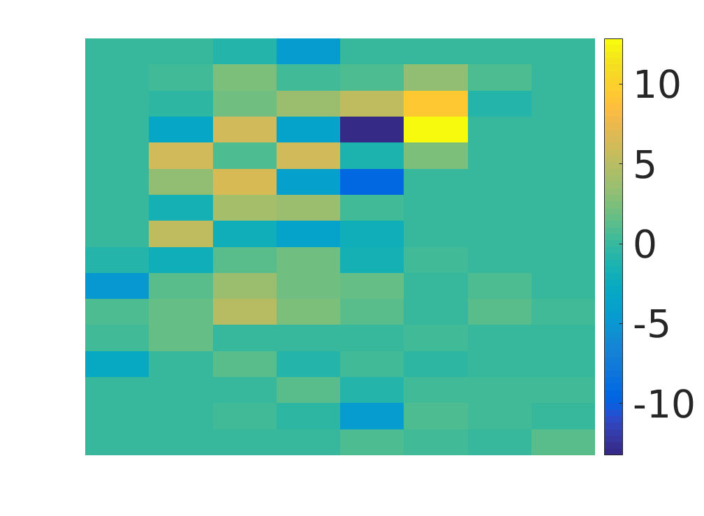
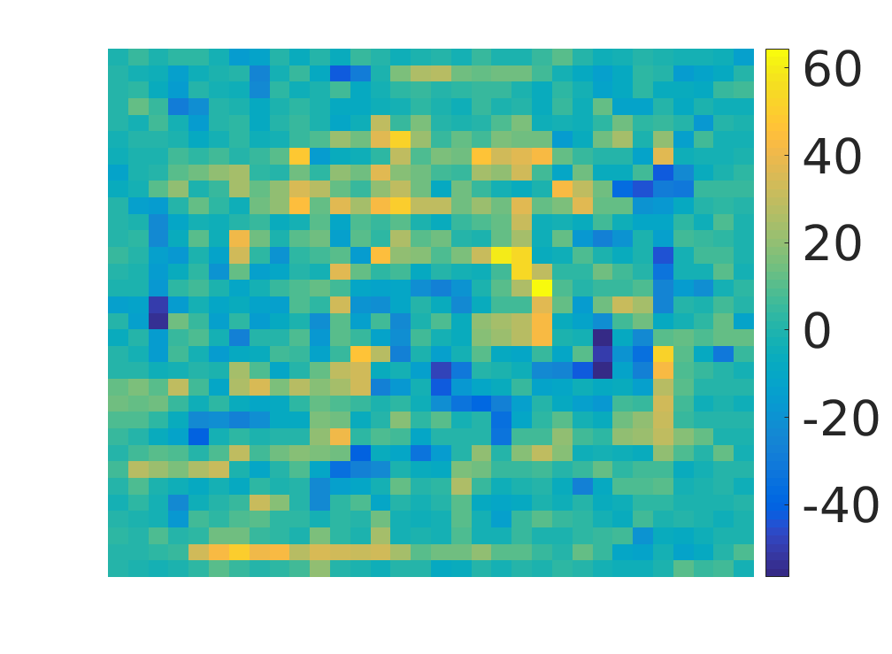
Due to the high condition number of the log-likelihood function with respect to the parameter $w$ (Zipkin:2016, ), we perform a simple grid search to find the optimal $w$ (see Fig. 5). The likelihood functions are maximized when $w$ is 20 and 18 for CHI and LA, respectively. The similarity between the optimal duration parameters for Chicago and Los Angeles suggest that the duration of the self-excitation is an intrinsic property of crime. The optimal self-excitation parameters sets $A$ for two cities are plotted in Fig.6. The diagonal in Fig. 6 reflects the intensity of self-excitation within a single node of the graph (i.e., zip code region). Off-diagonal entries reflects self-excitation of crime between nodes of the graph. Only nodes that demonstrate self-excitation above a threshold theta are connected by an edge in the final graph.

Figure 5. Plot of $w$ vs log-likelihood. The maximum value occurs at $w=20$ and $w=18$ respectively for CHI and LA.

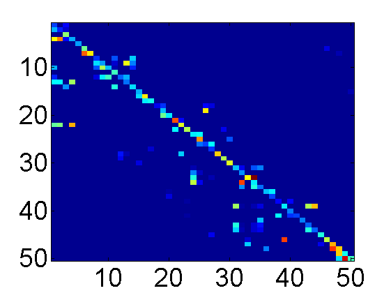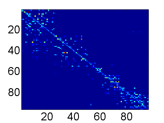(a) CHI	(b) LA

Figure 6. Image plot of the self and mutual excitation matrix $A$ for the cities CHI and LA.

3.1.2. Effectiveness of STWG Inference

We validate the efficacy of the inference algorithm on a synthetic problem. To generate the synthetic data, a random graph $G$ is first generated with a fixed level of sparsity on a fixed set of nodes $i=1,\dots,U$. A MHP $E$ is then simulated for a fixed amount of time $T$ with randomly generated background rate $\mu_{i}$, and excitation rates $a_{i,j}$ supported on the graph $G$. We use the aforementioned algorithm to infer the coefficients $\hat{a}_{i,j}$. To obtain the underlying graph structure, there is an edge connected from node $j$ to $i$ if and only if $\text{Sign}(\hat{a}_{i,j}-\theta)>0$, where $\theta$ is a threshold that determines the sparsity of the inferred weighted graph. To evaluate the efficacy of the inference algorithm, we vary the threshold $\theta$ to obtain a ROC curve, where a connection between two nodes $i$ and $j$ is treated as positive and vice versa. The area under the ROC curve (AUC) will be a metric on the performance of the algorithm.

For the experiments, we generate a directed and fully connected graph $G$ with $N=30$ nodes, and keep each edge $e_{ij}$ with probability $s=0.1,0.2,\dots,0.5$, where $s$ denotes the sparsity level of the graph. We generate at random $\mu_{i}\sim Unif([0,0.1])$ and $a_{i,j}\sim Unif([0.02,0.1])$ for $i,j$ connected in $G$, and $0$ otherwise. And we check the stability condition in the spectral norm where $\rho(A)<1$. A HP is then simulated with $T=3\times 10^{4}$. In crime networks, it is reasonable to assume that the interactions $a_{ij}$ are local, and hence we may start out with a reduced set of edges during the inference procedure to increase accuracy of the network recovery. Therefore, in addition to recovering the network structure from a fully connected graph, we also test the inference algorithm on a set of reduced edges that contain the ground truth. For simplicity, we randomly choose $200$ and $400$ edges from the graph and add them to the true network structure at initialization. We observe that the inference algorithm is able to obtain an AUC of around 0.9 across all levels of sparsity, with large increases in performance if the graph prior is narrower.

Table 1. AUC of the ROC curve for the graph inference problem. Rows denote the sparsity of the ground truth graph, columns are different prior knowledge for network structure for the inference algorithm.

Prior/Sparsity	0.1	0.2	0.3	0.4	0.5
Null	0.900	0.897	0.884	0.915	0.910
GT + 200	0.989	0.987	0.982	0.981	0.986
GT + 400	0.969	0.956	0.962	0.947	0.954

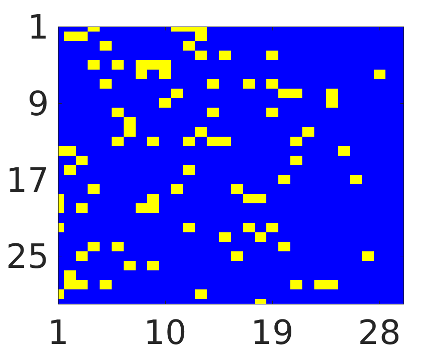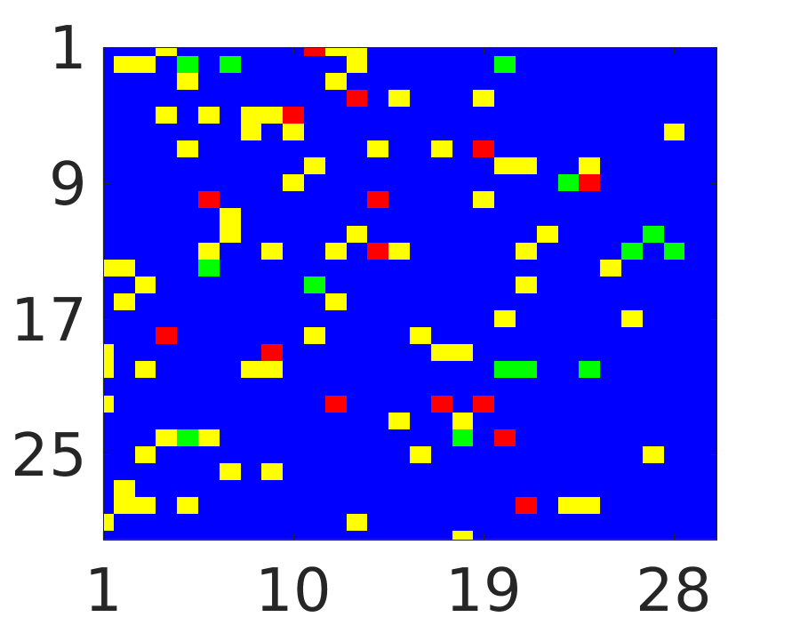(a) GT	(b) GT+200	(c) GT+400

Figure 7. Visualization of the ground truth and inferred graph for the synthetic data. The inferred graphs were obtained by thresholding $a_{ij}$ to match the sparsity level of the original network. The true positives, true negatives, false positives, false negatives are color coded in yellow, blue, red, green respectively.

3.2. Data Augmentation - Single Node Study

We consider data augmentation to boost the performance of the DNN for sparse data forecasting, with single zip code crime forecasting as an illustration. In our previous work (BaoWang:2017DL1, ; BaoWang:2017DL2, ), when dealing with crime forecasting on a square grid, we noticed the DNN poorly approximates the crime intensity function. However, it does approximate well the diurnal cumulated crime intensity, which has better regularity. According to the universal approximation theorem (Cybenko:1989, ), the DNN can approximate any continuous function with arbitrary accuracy. However, the crime intensity time series is far from a continuous function due to its spatial and temporal sparsity and stochasticity. Mathematically, consider the diurnal time series $\{x(t)\}$ with period $T$. We map $\{x(t)\}$ to its diurnal cumulative function via the following periodic mapping:

(4) $$y(t)=\int_{nT}^{t}x(s)ds\doteq I(x(t)),$$

for $t\in[nT,(n+1)T)$, this map is one-to-one.

We also super-resolve the diurnal cumulated time series $\{y(t)\}$ to constract an augmented time series $\{\hat{y}(T)\}$ on half-hour increments via linear interpolation. The new time series has a period of $\hat{T}=2T-1$. In the time interval $[n\hat{T},(n+1)\hat{T})$ it is defined as:

(5) $$\hat{y}(t)=\begin{cases}y(nT+k)&\text{$t=n\hat{T}+2k$}\\ \frac{1}{2}[y(nT+k)+y(nT+k+1)]&\text{$t=n\hat{T}+2k+1$,}\end{cases}$$

for $k=0,1,\cdots,T-1$. It is worth noting the above linear interpolation is completely local. In the following DNN training procedure it will not lead to information leak.

3.2.1. Cascaded LSTM for Single Node Crime Modeling

The architecture of the DNN used to model single node crime is a simple cascaded LSTM as depicted in Fig.8. The architecture contains two LSTM layers and one fully-connected (FC) layer, and represents the following function:

(6) $${\rm DNN}(x)={\rm FC}\circ{\rm LSTM}_{1}\circ{\rm LSTM}_{2}(x),$$

where $x$ is the input. Generally, we can cascade $N$ layers of LSTM.

Figure 8. The architecture of the cascaded LSTM that used for single node data modeling.

In the above cascaded architecture, all the LSTMs are equipped with 128 dimensional outputs except the first one with 64 dimensions. An FC layer maps the input tensor to the target value. To avoid information leak when applying DNN to the super-resolved time series, we skip the value at the nearest previous time slot in both training and generalization.

Before fitting the historical crime intensities by the cascaded LSTMs, we first look at histograms of the crime intensities (Fig.9). The 99th percentiles of crime distributions are each less than six crimes. This suggests that local crime intensity is important and one cannot use a simple binary classifier.

Figure 9. Histogram of the hourly crime counts in zip code regions 60620, for the year 2015, and 90003, for 2014-2015.

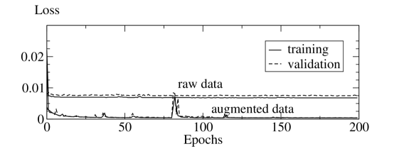
We adopt the two layers of LSTMs cascade, which is demonstrated in Fig.8 to fit the single node crime time series. To train the DNNs for a single node, we run 200 epochs with the ADAM optimizer (adam_15, ), starting from the initial learning rate 0.01 with decay rate $1e-6$. Fig. 10 shows the decay of the loss function for the raw crime time series and cumulated super-resolved (CS) time series in panels (a) and (b), respectively. It can be seen from the figure that DNN performs much better on the regularized time series than the raw one, i.e. the loss function reaches a much lower equilibrium.

Figure 10. Training procedures of the different scenarios on the node 90003. Evolution of the training and validation loss on the raw data and on the augmented data.

To show the advantage of the generalization ability of the DNN, we compare it with a few other approaches, including autoregressive integrated moving average (ARIMA), K-nearest neighbors (KNN), and historical average (HA). We use these models to fit the historical data and perform one step forecasting in the same manner as our previous work (BaoWang:2017DL2, ). The root mean squared error (RMSE) between the exact and predicted crime intensities and optimal parameters for the corresponding model are listed in Table 2. Under the RMSE measure, DNN, especially on the augmented data, yields higher accuracy. The small RMSE reflects the fact that DNN approximates the crime time series with good generalization ability.

Table 2. RMSE between the exact and predicted crime intensities over the last two months of 2015, in the region with zip code 90003. DNN(CS) denotes DNN model applied to the augmented data.

Methods	RMSE (number of crimes)
DNN	0.858
DNN (CS)	0.491
ARIMA(25, 0, 26)	0.941
KNN (k=1)	1.193
HA	0.904

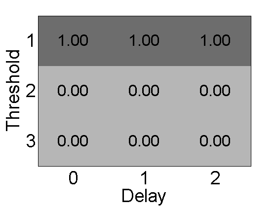
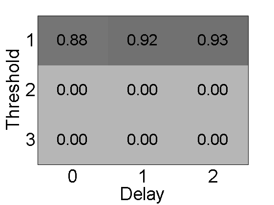
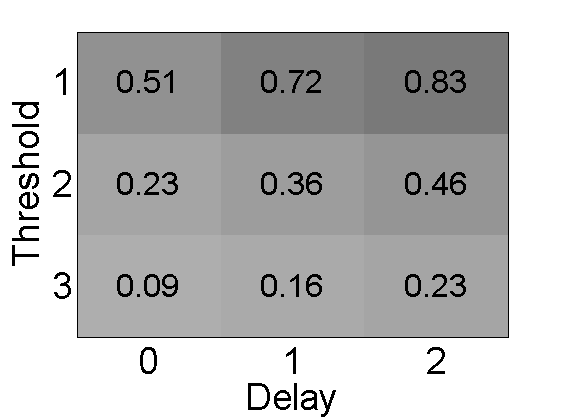
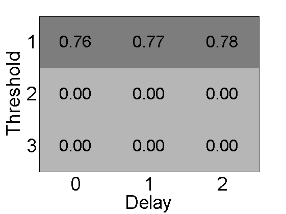
However, the simple RMSE measure is insufficient to measure error appropriately for sparse data. Do HA and ARIMA really work better than KNN for crime forecasting? HA ignores the day to day variation, while ARIMA simply predicts the number of crimes to be all zeros after flooring. KNN predicts more useful information than both ARIMA and HA for the crime time series. We propose the following measure, which we call a “precision matrix” (do not confuse it with the one used in statistics) $B$ be defined as:

$$B=\left(\begin{array}[]{ccc}\beta_{10}&\cdots&\beta_{1n}\\ \vdots&\vdots&\vdots\\ \beta_{m0}&\cdots&\beta_{mn}\\ \end{array}\right)$$

where $\beta_{ij}=\frac{N_{ij}}{N_{i}}$, where $N_{i}\doteq\#\{t|x_{t}\geq i\}$, and $N_{ij}\doteq\#\{t|x_{t}\geq i\ {\rm and}\ (x_{t}^{p}\geq i\ {\rm or}\ x_{t-1}^{p}\geq i\ {\rm or}\ \cdots\ {\rm or}\ x_{t-j+1}^{p}\geq i)\}$, for $i=1,2,\cdots n$; $j=0,1,\cdots,m$. Here $x_{t}$ and $x_{t}^{p}$ are the exact and predicted number of crimes at time $t$. This means for a given threshold number of crimes $i$, we count the number of time intervals in the testing set at which the predicted and exact number of crimes both exceed this threshold $i$, with an allowable delay $j$, i.e., the prediction is allowed within $j$ hours earlier than the exact time.

This measure provides much better guidance for crime patrol strategies. For instance, if we forecast more crime to occur in a given patrol area, then we can assign more police resources to that area. This metric allows for a few hours of delay but penalizes against crimes happening earlier than predicted, due to the time irreversibility of forecasting. For the crime time series in nodes 60620 and 90003, we select $m=3$, $n=2$ and $m=5$, $n=4$, respectively. Fig. 11 shows the precision matrices of the crime prediction by different methods, confirming that DNN together with data augmentation gives accurate crime forecasting. Meanwhile, the KNN also gives better results compared to other methods except the DNN with data augmentation. This corrects potential inaccuracies in the RMSE measure and confirms the spatial correlation of the crime time series.

Remark 1.

The precision matrix $B$ still has an issue in the case of over-prediction. Namely, this measure fails to penalize cases where the prediction is higher than the ground truth. However in those cases, the RMSE would typically be very large. Therefore, to determine if the sparse data is well predicted or not, we should examine both metrics.

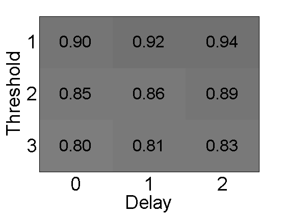(a) ARIMA	(b) HA	(c) KNN	(d) DNN original data	(e) DNN data augmentation

Figure 11. Precision matrix of the different predictors’s performance in forecasting crime in 90003.

Another merit of the DNN is that with sufficient training data, as the network goes deeper, better generalization accuracy can be achieved. To validate this, we test the 2 and 3 layers LSTM cascades on the node 60620 (see Fig. 12).

(a) 2-layer LSTM (RMSE 0.901)	(b) 3-layer STM (RMSE 0.648)

Figure 12. Precision matrix of the cascaded two and three layers LSTMs for crime zip code 60620, with RMSE.

3.3. GSRNN for ST Forecasting

(a)	(b)

Figure 13. Figure a) shows an example STWG inferred via the HP, where each color (red and green) denotes the class to which the node belongs. Figure b) depicts the feed-forward structure of our RNN network on a single node (node No.6).

Our implementation of the GSRNN is based on the SRNN implementation in (Jain:2016, ) (Fig.13), but differs in these key aspects: 1) We generalize the SRNN model to a directed graph, which is more suited to the ST data forecasting problem. 2) We use a weighted sum pooling based on the self-exciting weights from the MHP inference. 3) Due to the large number of nodes in the graph, we subsample each class of nodes for scalability.

To be more specific, suppose $i=1,2,\dots N$ are the nodes of the graph, and $X_{i}(t)$ denotes value of the time series at time $t$ for node $i$. We first deploy the STWG inference procedure to obtain the weighted directed graph, with weight on the edge connecting node $i$ and $j$ denoted as $w_{ij}$. With the same setup as in (Jain:2016, ), we partition the graph nodes to $K$ groups according to some criterion. We construct an “input RNN” $E^{1}_{k}$ for each class $k$, and an “edge RNN” $E^{2}_{k,l}$ for each class pair $(k,l)$ if $k\neq l$. For the forward pass, if node $i$ belongs to class $k$, we feed a set of historical data $\{X_{i}(t-p)|p=n_{1},n_{2},...,n_{m}\}$ to $E^{1}_{k}$, and the data from neighboring nodes of class $l$ to $E^{2}_{k,l}$. In contrast to (Jain:2016, ), we use a weighted sum pooling for the edge inputs, i.e., $X^{\prime}_{i}=\sum_{j,cl(j)=k}w_{i,j}X_{j}$. This pooling has shown to be more suitable for ST data forecasting. Finally, the output from the two RNNs are concatenated and fed to a node RNN $N^{1}_{j}$, which then predicts the number of events at time $t$. For each epoch during training, we can also sample the nodes to maintain scalability when dealing with large graphs. The sampling can be done non-uniformly across groups, e.g., sampling more often groups that contribute higher to the overall error.

Algorithm 1 GSRNN for ST Forecasting.

Input: Input crime intensity $\{x_{i}(t)\}_{t=1}^{n}$, for all nodes $i=1\dots N$.

Output: Predicted crime intensity $x_{t}(i)$ at time slot $t=n+1$ for all nodes $i$.

Step 1: Infer the mutual excitation coefficient using the Hawkes model $w_{ij}$ for the multivariate time series $x_{t}(i)$, and set as graph weights.

Step 2: Partition the nodes to $K$ classes according to total crime count.

Step 3: Preprocess each time series $x_{t}(i)$ by apply superresolution and integration as in Eqns .(4) and (5).

Step 4: Construct GSRNN model where the edge RNN outputs are pooled via a weighted sum $\sum_{cl(j)=c}w_{ij}x_{j}$.

Step 5: Train network via ADAM, optionally subsample the nodes in each class for efficiency.

Step 6: Apply the inverse maps to the data augmentation to recover the predicted crime intensity at the time $n+1$.

4. ST Crime Forecasting Results

We compare two naive strategies that do not utilize the STWG information against the GSRNN model. The first, denoted by Single Node, trains a separate LSTM model on each individual zip code. The second, denoted as Joint Training, organizes the zip code regions in three groups according to the average crime rate (Group1 contains the zip code regions with lowest crime rate, and so forth.). The RNN is trained jointly for each group.

To construct the STWG used in the GSRNN model, a K-nearest neighbor graph of $K=15$ is used as the initial sparse structure for the MHP inference algorithm. The obtained self excitation rates $a_{ij}$ are further thresholded to reach a sparsity rate of 0.1, and then normalized. Namely, $w_{ij}=\frac{a_{ij}}{max(a_{ij})}$.

For both single node and joint training, a 2-layer LSTM with 128 and 64 units is used, where a dropout rate of 0.2 is applied to the output of each layer. For the GSRNN model, a 64/128 unit single layer LSTM is used for the edge/node RNN, respectively.

All models are trained using the ADAM optimizer with a learning rate of 0.001 and other default parameters. We compare the RMSE in both CDF (diurnal cumulated time series) and PDF (raw time series) of the predictions. For the LA Data, we test on the last two months, and use the rest for training. For CHI we test on the last one month (31 days), and use the rest for training. See Tables 3 and 4.

Table 3. Average RMSE on for LA Crime Data. Left: RMSE on CDF, Right: RMSE on PDF.

	Single Node	Joint Training	GSRNN
Group 1	0.108/0.113	0.062/0.075	0.059/0.078
Group 2	0.154/0.165	0.102/0.124	0.082/0.109
Group 3	0.235/0.251	0.168/0.191	0.144/0.183
Average	0.174/0.185	0.120/0.140	0.103/0.131

Table 4. Average RMSE on for CHI Crime Data. Left: RMSE on CDF, Right: RMSE on PDF. Unit: number of crimes.

	Single Node	Joint Training	GSRNN
Group 1	0.174/0.166	0.204/0.143	0.102/0.108
Group 2	0.381/0.348	0.153/0.133	0.181/0.197
Group 3	0.699/0.697	0.413/0.495	0.382/0.412
Average	0.482/0.471	0.286/0.317	0.258/0.278

(a) Los Angeles	(b) Chicago

Figure 14. Precision matrix of GSRNN for Los Angeles and Chicago averaged across top all zipcodes with at least one hourly time slot containing more than 3 crimes.

(a)CHI zip code 60171	(b)LA zip code 90003

Figure 15. Panels a), b) plot snapshots of the predicted vs exact hourly crime rate for CHI and LA data.

We observe that Joint Training leads to a performance boost compared to the Single Node approach, and adding the bidirectional graph leads to a further performance increase. Theses conclusions are consistent across the stratified groups as well. The precision matrices (thresholded to three in both number of crimes and delay) averaged over all the nodes for LA and CHI are plotted in Fig. 14, respectively. Figure 15 shows the predicted and exact crime time series over two graph nodes.

5. ST Traffic Forecasting Results

We benchmark our methodology on two public datasets for traffic forecasting (Junbo:2017, ). The BikeNYC and TaxiBJ datasets are both embedded in rectangular bounding boxes, forming a rectangular grid of size 32 x 32 and 16 x 8 respectively.

To cast the problem into the graph representation framework used in this paper, we consider each pixel in the spatial grid as a graph node, and connect each node with its four immediate neighbors. The graph weights are set to $1/4$ for all edges, the same as in an unweighted graph. More sophisticated methods could be used for graph construction, but we found the 4-regular graph already yields good performance. The nodes are then sorted into three classes according to the overall cumulative traffic count. For the New York data, there are three equal size classes, whereas in the Beijing dataset, the classification is picked manually to reflect the geographical structure of the Beijing road system (see Fig. 16).

(a)	(b)	(c)

Figure 16. Panels a)-c) visualize the node class assignment from group 1 - 3 in the Beijing Traffic data respectively, where a yellow pixel indicates the assignment of the pixel node to its corresponding class. For example, the yellow pixels in panel a) are grouped to class 1.

For the BikeNYC, we use a two layer LSTM with (32, 64) units and 0.2 dropout rate at each layer for the single-node model, and a two layer LSTM with (64, 128) units and 0.2 dropout rate at each layer for the joint and GSRNN model. For the TaxiBJ, we use a two layer LSTM with (64,128) units for the single-node, and a three layer LSTM model with (64, 128, 64) units for the joint model; for the GSRNN model, the edge RNN is a two layer LSTM with (64, 128) units, and the node RNN is a one layer LSTM with 128 units. All models are trained using the ADAM optimizer with a learning rate of 0.001 and other default parameters. The learning rate is halved every 50 epochs, and a total of 500 epochs is used for training.

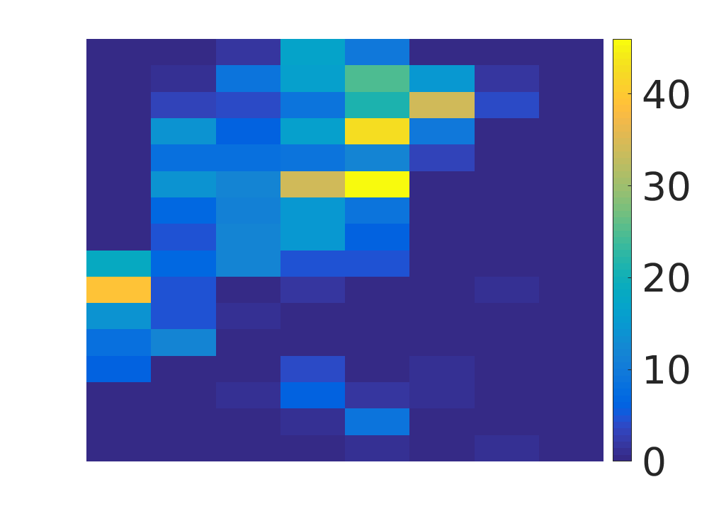
For evaluation, we use the Root Mean Square Error (RMSE) across all nodes and all time intervals. The same train-test split is used in our experiments as in (Junbo:2017, ). The results on RMSE (Table 5) are reported on the testing error based on the model parameters with the best validation loss. Comparisons between the predicted and exact traffic on two grids over a randomly selected time period is shown in Fig. 17. On a randomly selected time slot, we plot the predicted and exact spatial data and errors in Figs. 18 and 19.

Table 5. RMSE on for Traffic Data.

	Single	Joint	GSRNN	STResNet
	Node	Training		(Junbo:2017, )
Beijing	23.50	19.5	16.59	16.69
NY	6.77	6.33	6.08	6.33

New York: $x=(5,5)$	Beijing: $x=(12,7)$

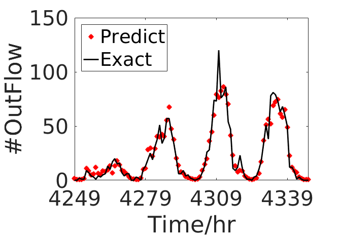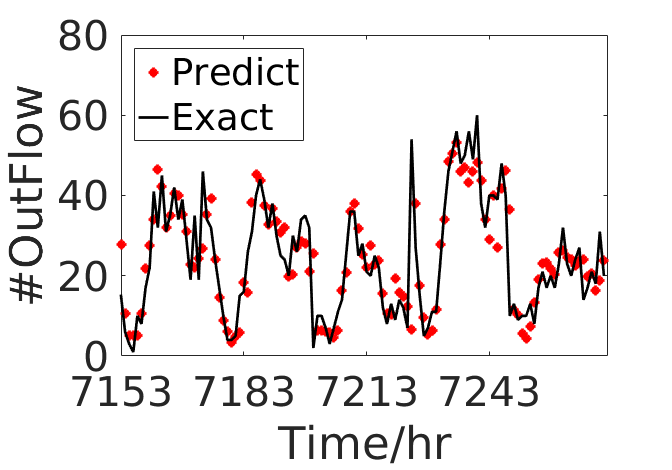Figure 17. Comparison between predicted vs exact traffic out-flow at a specified point $x$ for New York and Beijing.

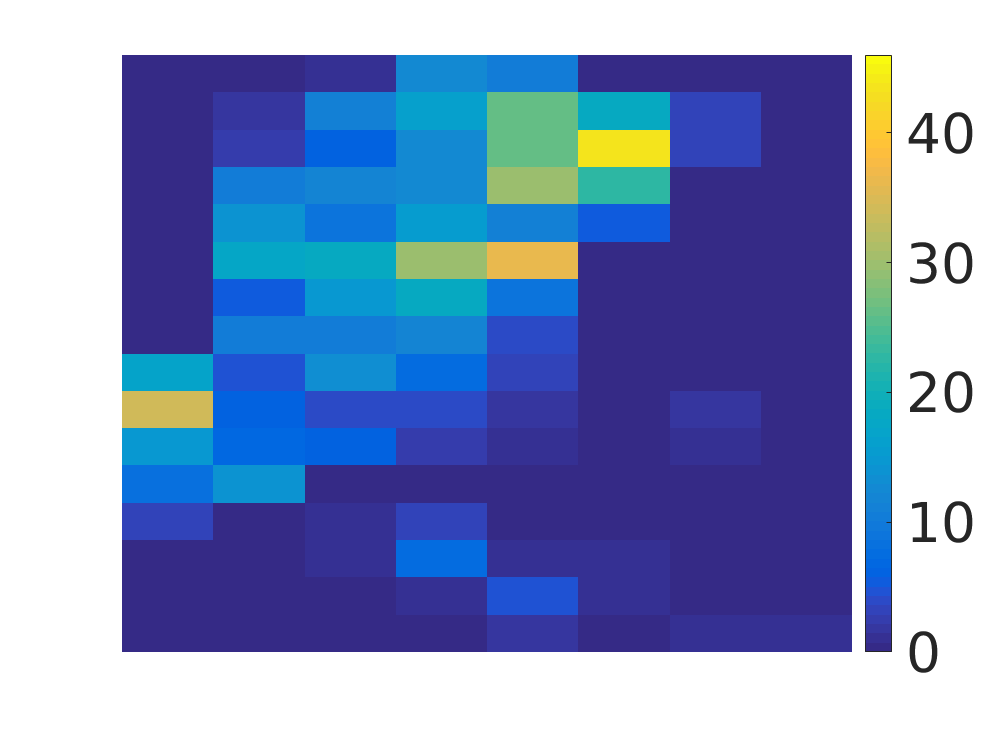(a) predicted	(b) exact	(c) difference

Figure 18. Comparison between predicted (a) and exact (b) traffic out-flow at $t=8647$ for New York city over a $16\times 8$ grid. Difference shown in c).

(a) predicted	(b) exact	(c) difference

Figure 19. Comparison between predicted (a) and exact (b) traffic out-flow at $t=17204$ for Beijing over a $32\times 32$ grid. Difference shown in (c).

6. Conclusion

We develop a multiscale framework that contains two components: inference of the macroscale spatial temporal graph representation of the data, and a generalizeable graph-structured recurrent neural network (GSRNN) to approximate the time series on the STWG. Our GSRNN is arranged like a feed forward multilayer perceptron with each node and each edge associated with LSTM cascades instead of weights and activation functions. To reduce the model’s complexity, we apply weight sharing among certain type of edges and nodes. This specially designed deep neural network (DNN) takes advantage of the RNN’s ability to learn the pattern of time series, capturing real time interactions of each node to its connected neighbors. To predict the value of the time series for a node at the next time step, we use the information of its neighbors and real time interactions. For the ST sparse data, we propose efficient data augmentation techniques to boost the DNN’s performance. Our model demonstrates remarkable results on both crime and traffic data; for crime data we measure the performance with both root mean squared error (RMSE) and the proposed precision matrix.

The method developed here forecasts crime on the time scale of an hour in each US zip code region. This is in contrast to the commercial software PredPol (www.predpol.com) that forecasts on a smaller spatial scale and longer timescale. Due to the different scales, the methods have different uses - PredPol is used to target locations for patrol cars to disrupt crime whereas the method proposed here might be used for resource allocation on an hourly basis within different patrol regions.

There are a few issues that require future attention. The space on which the data is distributed is represented as a static graph. A dynamic graph that better models the changing mutual influence between neighboring nodes could be incorporated in our framework. Furthermore, in the traffic forecasting problem, better spatial representation of the traffic data could also be explored. Our model could also be applied to broader fields, e.g., quantitative finance and social networks (Zipkin:2016, ).

7. Acknowledgments

This work was supported by ONR grant N00014-16-1-2119 and NSF DMS grants 1417674 and 1737770. The authors thank the Los Angeles Police Department for providing the crime data. We thank Dr. Da Kuang for help with the QGIS software.

References

- (1) G. Cybenko. Approximations by superpositions of sigmoidal functions. Mathematics of Control, Signals, and Systems, 2(4):303–314, 1989.
- (2) N. Du, H. Dai, R. Trivedi, U. Upadhyay, M. Rodriguez, and L. Song. Recurrent marked temporal point process. KDD, 2016.
- (3) T. Goldstein and S.J. Osher. The split bregman method for l1-regularized problems. SIAM journal on imaging sciences, 3(2):323–343, 2009.
- (4) K. He, X. Zhang, S. Ren, and J. Sun. Deep residual learning for image recognition. CVPR, 2016.
- (5) S. Hochreiter and J. Schmidhuber. Long short-term memory. Neural Comput., (9):1735–1780, 1997.
- (6) D. Holden, T. Komura, and J. Saito. Phase-functioned neural networks for character control. Siggraph, 2017.
- (7) A. Jain, A. R. Zamir, S. Savarese, and A. Saxena. Structural-rnn: Deep learning on spatio-temporal graphs. CVPR, 2016.
- (8) H. Kang and H. Kang. Prediction of crime occurrence from multi-modal data using deep learning. PLos ONE, (12), 2017.
- (9) D. Kingma and J. Ba. Adam: A method for stochastic optimization. ICLR, 2015.
- (10) P. J. Laub, T. Taimre, and P. K. Pollett. Hawkes processes. arXiv:1507.02822, 2015.
- (11) Y. LeCun, Y. Bengion, and G. Hinton. Deep learning. Nature, (521):436–444, 2015.
- (12) Y. Li, R. Zemel, M. Brockschmidt, and D. Tarlow. Gated graph sequence neural network. ICLR, 2016.
- (13) G. Mohler, M. Short, S. Malinowski, M. Johnson, G.E. Tita, A.L. Bertozzi, and P. J. Brantingham. Randomized controlled field trials of predictive policing. Journal of Americal Statistical Association, 111(512):1399–1411, 2015.
- (14) G. O. Mohler, M. B. Short, and P. J. Brantingham. The concentration dynamics tradeoff in crime hot spotting. Connecting Crime to Place: New Directions in Theory and Policy, 2018.
- (15) QGIS Development Team. Qgis geographic information system. Open Source Geospatial Foundation, 2009.
- (16) A. Veen and F. P. Schoenberg. Estimation of space-time branching process models in seismology using an em-type algorithm. JASA., 103(482):614–624, 2008.
- (17) B. Wang, P. Yin, A. L. Bertozzi, P. J. Brantingham, S. J. Osher, and J. Xin. Deep learning for real time crime forecasting and its ternization. arXiv:1711.08833, 2017.
- (18) B. Wang, D. Zhang, D. Zhang, P. J. Brantingham, and A. L. Bertozzi. Deep learning for real time crime forecasting. International Symposium on Nonlinear Theory and Its Applications (NOLTA), Cancun, Mexico, pages 330–333, 2017.
- (19) J. Zhang, Y. Zheng, and D. Qi. Deep spatio-temporal residual networks for citywide crowd flows prediction. AAAI, 2017.
- (20) K. Zhou, H.Y. Zha, and L. Song. Learning social infectivity in sparse low-rank networks using multi-dimensional hawkes processes. AISTATS, 2013.
- (21) J. R. Zipkin, F.P. Schoenberg, K. Coronges, and A. L. Bertozzi. Point-process models of social network interactions: parameter estimation and missing data recovery. Eur. J. Appl. Math., pages 502–529, 2016.