CLUMP-3D: Three-dimensional Shape and Structure of 20 CLASH Galaxy Clusters from Combined Weak and Strong Lensing

Abstract

We perform a three-dimensional triaxial analysis of 16 X-ray regular and 4 high-magnification galaxy clusters selected from the CLASH survey by combining two-dimensional weak-lensing and central strong-lensing constraints. In a Bayesian framework, we constrain the intrinsic structure and geometry of each individual cluster assuming a triaxial Navarro–Frenk–White halo with arbitrary orientations, characterized by the mass $M_{200\mathrm{c}}$, halo concentration $c_{200\mathrm{c}}$, and triaxial axis ratios ($q_{\mathrm{a}}\leqslant q_{\mathrm{b}}$), and investigate scaling relations between these halo structural parameters. From triaxial modeling of the X-ray-selected subsample, we find that the halo concentration decreases with increasing cluster mass, with a mean concentration of $c_{200\mathrm{c}}=4.82\pm 0.30$ at the pivot mass $M_{200\mathrm{c}}=10^{15}\mathrm{M}_{\odot}\,h^{-1}$. This is consistent with the result from spherical modeling, $c_{200\mathrm{c}}=4.51\pm 0.14$. Independently of the priors, the minor-to-major axis ratio $q_{\mathrm{a}}$ of our full sample exhibits a clear deviation from the spherical configuration ($q_{\mathrm{a}}=0.52\pm 0.04$ at $10^{15}\mathrm{M}_{\odot}\,h^{-1}$ with uniform priors), with a weak dependence on the cluster mass. Combining all 20 clusters, we obtain a joint ensemble constraint on the minor-to-major axis ratio of $q_{\mathrm{a}}=0.652^{+0.162}_{-0.078}$ and a lower bound on the intermediate-to-major axis ratio of $q_{\mathrm{b}}>0.63$ at the $2\sigma$ level from an analysis with uniform priors. Assuming priors on the axis ratios derived from numerical simulations, we constrain the degree of triaxiality for the full sample to be $\mathcal{T}=0.79\pm 0.03$ at $10^{15}\mathrm{M}_{\odot}\,h^{-1}$, indicating a preference for a prolate geometry of cluster halos. We find no statistical evidence for an orientation bias ($f_{\mathrm{geo}}=0.93\pm 0.07$), which is insensitive to the priors and in agreement with the theoretical expectation for the CLASH clusters.

1. Introduction

Galaxy clusters are gravitationally dominated by dark matter and serve as a wealth of ideal laboratories to study structure formation in the universe. In particular, an accurate mass estimation of galaxy clusters is crucial not only for utilizing them as cosmological probes (Planck Collaboration et al., 2015; Mantz et al., 2015; Bocquet et al., 2015; de Haan et al., 2016) but also for understanding the root cause of various astrophysical processes in massive halos, such as environmental quenching of galaxies (Dressler, 1980). Conventionally, the total cluster mass is determined from projected measurements assuming spherical symmetry. In this context, $N$-body simulations in the standard $\Lambda$ cold dark matter ($\Lambda\textrm{CDM}$) model established a nearly self-similar form for the spherically averaged density profile $\rho(r)$ of dark-matter halos (Navarro et al., 1996), which can be characterized by two parameters, namely the characteristic density and radius of halos. This two-parameter model gives a satisfactory success in terms of statistically quantifying the ensemble mass of observed clusters over a sizable sample (e.g., Umetsu et al., 2011a; Newman et al., 2013; Umetsu et al., 2014; von der Linden et al., 2014; Hoekstra et al., 2015; Umetsu et al., 2016; Okabe & Smith, 2016).

However, cluster halos are predicted to be non-spherical, with a preference for prolate shapes according to $N$-body simulations in the $\Lambda\textrm{CDM}$ model (Frenk et al., 1988; Dubinski & Carlberg, 1991; Warren et al., 1992; Jing & Suto, 2002). Besides, the shape of halos is predicted to depend on the redshift, halo mass, and cluster-centric radius (Bailin & Steinmetz, 2005; Hopkins et al., 2005; Allgood et al., 2006; Bett et al., 2007; Bonamigo et al., 2015), as well as on baryonic effects (Flores et al., 2007), large-scale environments (Kasun & Evrard, 2005), and the background cosmology (Allgood et al., 2006; Despali et al., 2014). Therefore, cluster mass estimates assuming spherical symmetry cause a substantial scatter around their true mass (e.g., Battaglia et al., 2011). Importantly, an inappropriate assumption about the cluster shape and orientation could significantly bias individual mass measurements (e.g., Oguri et al., 2005). There have been initial attempts to compare the observed shapes of galaxy clusters with those predicted by cosmological numerical simulations (e.g., Oguri et al., 2010), opening up a new avenue of testing models of structure formation. It is thus important to perform a statistical analysis of the shape of clusters by extending cluster mass determinations beyond spherical modeling.

Compared to the theoretical efforts to characterize the shape of galaxy clusters in numerical simulations, significantly less progress has been made on the observational side (De Filippis et al., 2005; Sereno et al., 2006; Corless et al., 2008; Morandi & Limousin, 2012; Limousin et al., 2013; Umetsu et al., 2015; Sereno et al., 2017b). Detailed observational work thus far was subject to case studies instead of a statistical interpretation from a large cluster sample, because of difficulty in acquiring data sets that are needed to achieve the required precision. Moreover, the shape of the total mass distribution in clusters was often inferred indirectly from observations of the intracluster medium (ICM) assuming hydrostatic equilibrium, which however would be violated in the presence of, for example, turbulent and bulk motions of hot gas (Lau et al., 2009; Molnar et al., 2010; Chiu & Molnar, 2012). Astrophysical processes, such as radiative cooling of ICM and entropy injection from active galactic nuclei, as well as the cluster dynamical state (Cialone et al., 2017), further complicate the interpretation of cluster shapes inferred from X-ray or the Sunyaev–Zel’dovitch Effect (SZE hereafter; Sunyaev & Zel’dovich, 1970, 1972) observations. Thus, investigating the shape of galaxy clusters is observationally challenging.

Gravitational lensing provides a direct access to the underlying mass distribution of galaxy clusters without requiring any assumptions about their dynamical or physical state. There have been many successful attempts to determine the cluster mass by weak lensing (Okabe et al., 2010; von der Linden et al., 2014; Hoekstra et al., 2015; Melchior et al., 2017; Medezinski et al., 2017; Schrabback et al., 2018), strong lensing (Broadhurst et al., 2005b; Richard et al., 2010; Zitrin et al., 2015; Grillo et al., 2015) and the combination of both (Bradač et al., 2006; Oguri et al., 2012; Umetsu, 2013; Umetsu et al., 2016). With recent progress in controlling systematics in weak lensing (e.g., intensive calibration against simulations; Bridle et al., 2010; Kitching et al., 2012; Mandelbaum et al., 2015), together with advances in instrumentation and observing techniques, we are in a great position to utilize gravitational lensing with high-quality lensing data.

In this work, we aim to use both weak and strong lensing to constrain the three-dimensional (3D) structure and shape of clusters targeted by the CLUster Multi-Probes in Three Dimensions (CLUMP-3D) program (Sereno et al., 2017b). Our sample consists of 20 high-mass clusters that were selected by the Cluster Lensing And Supernova survey with Hubble (CLASH, hereafter; Postman et al., 2012). Importantly, these 20 clusters were all deeply followed up from the ground and from space in different wavelengths (Donahue et al., 2014; Umetsu et al., 2014; Rosati et al., 2014; Czakon et al., 2015), with the goal of precisely characterizing the cluster mass distribution. Besides, these clusters have been intensively studied in previous work in the context of galaxy evolution (Annunziatella et al., 2014; DeMaio et al., 2015; Gupta et al., 2016), characterization of strongly lensed arcs (Zitrin et al., 2015), wide-field weak-lensing analysis (Umetsu et al., 2012, 2014), and exploration of the high-redshift universe (Zheng et al., 2012; Coe et al., 2013; Balestra et al., 2013; Monna et al., 2014; McLeod et al., 2016).

In the first paper of the CLUMP-3D program, Sereno et al. (2017b) carried out a full triaxial analysis of MACS J1206.2$-$0847 using multi-probe data sets from weak-lensing, strong-lensing, X-ray, and SZE observations, demonstrating the power of multi-probe cluster analysis. In our companion paper, Umetsu et al. (2018) present direct reconstructions of the two-dimensional (2D) matter distribution in the 20 CLASH clusters from a joint analysis of 2D shear and azimuthally averaged magnification measurements. This work is the third paper of the series, where we focus on characterizing the 3D mass distribution of the 20 CLASH clusters by combining weak and strong lensing. A multi-probe triaxial analysis of 16 X-ray-selected CLASH clusters using weak-lensing, strong-lensing, X-ray, and SZE data sets is presented in another companion paper (Sereno et al., 2018). We note that even though a joint analysis of multi-probe data sets can formally achieve a better precision, studies using gravitational lensing alone have the advantage of being free from assumptions about baryonic components in clusters. Therefore, both approaches are required and complementary to each other.

This paper is organized as follows. We will briefly introduce the basics of gravitational lensing in Section 2. We then describe the cluster sample and the lensing data products in Section 3. In Section 4 we outline our methodology for triaxial modeling. We discuss our results in Section 5, followed by the conclusions made in Section 6. Throughout this work, we assume a flat $\Lambda\textrm{CDM}$ cosmological model with $\Omega_{\mathrm{m}}=0.27$, $H_{0}=h\times 100$ km s ^-1Ṁpc^-1 with $h=0.7$, and $\sigma_{8}=0.8$. We define an ellipsoidal overdensity radius $R_{\Delta}$ (e.g., Corless et al., 2009; Umetsu et al., 2015) such that the mean interior density contained within an ellipsoidal volume of semimajor axis $R_{\Delta}$ is $\Delta$ times the critical density of the universe $\rho_{\mathrm{c}}(z)$ at the cluster redshift $z$. We use $\Delta=200$ to define the halo mass, $M_{\mathrm{200c}}$. All quoted errors are $68\%$ confidence limits (i.e., $1\sigma$) unless otherwise stated. We use the AB magnitude system. The notation $\mathcal{U}(x,y)$ stands for a uniform distribution between $x$ and $y$.

2. Theory of Gravitational Lensing

In this section, we briefly review the basics of gravitational lensing with emphasis on cluster lensing. In this case, we can approximate the lensing cluster of interest at redshift $z_{\mathrm{d}}$ as a single thin lens embedded in a homogeneous universe where background sources at redshift $z>z_{\mathrm{d}}$ are all lensed. We refer the readers to Bartelmann & Schneider (2001), Umetsu (2010) and Hoekstra et al. (2013) for a more complete overview of gravitational lensing.

To the first order, the deformation of observed background images due to gravitational lensing can be described by the lensing Jacobian matrix (see Equation (1)), which is characterized by the convergence $\kappa$ and the shear $\gamma\equiv\gamma_{1}+i\gamma_{2}$ at the position $\bm{\vartheta}$ on the lens plane,

$$J(\bm{\vartheta})=\begin{pmatrix}1-\kappa-\gamma_{1}&-\gamma_{2}\\ -\gamma_{2}&1-\kappa+\gamma_{1}\end{pmatrix},$$ (1)

where $\kappa$, $\gamma_{1}$, and $\gamma_{2}$ are written as linear combinations of second derivatives of the lensing potential. The convergence $\kappa(\bm{\vartheta})$ is the surface mass density normalized by the critical surface mass density for lensing $\Sigma_{\mathrm{c}}$,

$$\kappa(\bm{\vartheta})=\frac{\Sigma(\bm{\vartheta})}{\Sigma_{\mathrm{c}}},$$ (2)

where $\Sigma(\bm{\vartheta})$ is the surface mass density of the cluster projected along the line of sight, and

$$\Sigma_{\mathrm{c}}=\frac{c^{2}}{4\pi G}\frac{D_{\mathrm{s}}}{D_{\mathrm{l}}D_{\mathrm{ls}}}$$ (3)

with $G$ the Newton’s constant, and $D_{\mathrm{l}}$, $D_{\mathrm{s}}$ and $D_{\mathrm{ls}}$ the angular diameter distances between the observer-to-cluster, observer-to-source, and the cluster-to-source pairs, respectively. The complex shear $\gamma$ is related to the convergence $\kappa$ by

$$\gamma(\bm{\vartheta})=\int\mathrm{d}^{2}\bm{\vartheta^{\prime}}D(\bm{\vartheta}-\bm{\vartheta^{\prime}})\kappa(\bm{\vartheta^{\prime}}),$$ (4)

where the convolution kernel is defined as $D(\bm{y})\equiv\left(y_{2}^{2}-y_{1}^{2}-2iy_{1}y_{2}\right)/(\pi|\bm{y}|^{4})$.

In general, the observable quantity for weak lensing is not the gravitational shear $\gamma$  but the reduced shear $g$ in the subcritical regime,

$$g=\frac{\gamma}{1-\kappa}.$$ (5)

The reduced shear $g$ remains invariant under the global transformation, $\kappa\rightarrow\lambda\kappa+1-\lambda$ and $\gamma\rightarrow\lambda\gamma$, for any $\lambda\neq 0$. This is referred to as the mass-sheet degeneracy (Bartelmann & Schneider, 2001), which can be broken, for example, by including the lensing magnification effect.

The lensing magnification is characterized by the inverse determinant of the Jacobian matrix,

$$\mu=\frac{1}{\left(1-\kappa\right)^{2}-|\gamma|^{2}}.$$ (6)

The magnification factor transforms differently as $\mu\rightarrow\lambda^{-2}\mu$, which can be used to break the mass-sheet degeneracy. In the subcritical regime where $\mu>0$ and $|g|<1$, the magnification introduces two competing effects: the reduction (increase) of observed area on the source plane given a solid angle, and the amplificatin (deamplification) of flux of background sources. As a net result, the surface number density of a “flux-limited” background sample is altered due to the presence of lensing magnification depending on the intrinsic slope of the background luminosity function. This effect is known as magnification bias (Broadhurst et al., 1995; Taylor et al., 1998).

The effect of magnification bias can be measured by comparing cumulative number counts of flux-limited background galaxies with and without gravitational lensing as

$$\mu^{2.5s-1}=\frac{n(<m)}{n_{0}(<m)},$$ (7)

where $n(<m)$ and $n_{0}(<m)$ represent the lensed and unlensed surface number densities of background galaxies brighter than the apparent magnitude $m$, respectively, and $s\equiv\mathrm{d}\log n_{0}(<m)/\mathrm{d}{m}$ is the logarithmic slope of the cumulative magnitude distribution. It has been shown that, with a sizable sample of galaxy clusters, this effect can be solely used to calibrate the cluster mass proxies (e.g., Hildebrandt et al., 2009; Ford et al., 2012; Chiu et al., 2016a; Tudorica et al., 2017). By combining complementary observables of shear and magnification, one can break the mass-sheet degeneracy (Broadhurst et al., 2005a; Umetsu & Broadhurst, 2008). In this work, we combine both observables to derive an unbiased convergence map for each individual cluster (see Section 3.2).

In the regime of strong lensing, detailed modeling with many sets of multiple images with known redshifts allows to determine the location of critical curves, which then returns robust estimates of the Einstein mass, that is, the projected mass enclosed by the critical area $A_{\mathrm{c}}$ of an effective Einstein radius $\theta_{\mathrm{Ein}}=\sqrt{A_{\mathrm{c}}/\pi}$ (Zitrin et al., 2015),

$$M_{\mathrm{SL}}(<r)=\Sigma_{\mathrm{c}}{D_{\mathrm{l}}}^{2}\int_{|\bm{\vartheta}|\leq r}\kappa(\mathbf{\bm{\vartheta}})\mathrm{d}^{2}\mathbf{\bm{\vartheta}}.$$ (8)

In this work, we use strong-lensing constraints in the form of the enclosed projected mass profile around the effective Einstein radius. These constraints were obtained by Umetsu et al. (2016) using detailed lens models constructed by Zitrin et al. (2015) from a combined strong and weak lensing analysis of Hubble Space Telescope (HST) observations. We give further details in Section 3.3.

3. Cluster Sample and Data

We first describe the cluster sample in Section 3.1. The data products of weak and strong lensing are presented in Section 3.2 and Section 3.3, respectively.

3.1. Cluster Sample

In this work, we study a sample of 16 X-ray regular and 4 high-magnification galaxy clusters targeted by the CLUMP-3D program (Sereno et al., 2017b, 2018; Umetsu et al., 2018). Our sample stems from the CLASH wide-field weak-lensing analysis of Umetsu et al. (2014), and comprises two subsmples, both taken from the CLASH survey (Postman et al., 2012) targeting 25 high-mass clusters. Here, 20 clusters in the first CLASH subsample were selected to have X-ray temperatures greater than 5 keV and to have regular X-ray morphology. Numerical simulations suggest that this subsample is largely composed of relaxed clusters and free of orientation bias (Meneghetti et al., 2014). The second subset of 5 clusters were selected for their high magnification properties. These clusters turn out to be dynamically disturbed, merging systems (Zitrin et al., 2013; Medezinski et al., 2013; Balestra et al., 2016; Jauzac et al., 2017). Accordingly, modeling with a single-halo component may not be adequate to describe the high-magnification subsample (Medezinski et al., 2013), in contrast to the X-ray-selected subsample that can be well described by a single Navarro–Frenk–White (Navarro et al., 1997, hereafter NFW) profile out to large cluster radii (Umetsu et al., 2016; Umetsu & Diemer, 2017). For the sake of homogeneity, however, we analyze all clusters in the full sample in a consistent manner. We will also split the sample into several subsamples and statistically characterize each of them (see Section 4.3).

This sample spans a factor of $\approx 5$ in mass ($4\times 10^{14}\mathrm{M}_{\odot}\,h^{-1}<M_{200\mathrm{c}}<20\times 10^{14}\mathrm{M}_{\odot}\,h^{-1}$; Umetsu et al., 2016) and a redshift range of $0.18<z<0.69$. Following Umetsu et al. (2014), we adopt the location of the brightest cluster galaxy (BCG) as the center for each cluster. As discussed in Umetsu et al. (2014), the rms of positional offsets between the BCGs and X-ray peaks for the full sample is $\approx 30$ kpc $h^{-1}$, and it reduces to $\lesssim 10$ kp $h^{-1}$ for the X-ray-selected subsample. Therefore, the effect of miscentering is not expected to be significant in this work (Johnston et al., 2007; Umetsu et al., 2011b, 2016). We tabulate the basic information of our 20 clusters in Table 3.1.

We note that this sample has been intensively studied in previous CLASH work, especially by Umetsu et al. (2014, hereafter U14) and Umetsu et al. (2016, hereafter U16), who performed recnstructions of the azimuthally averaged surface mass density profile from weak and weak+strong lensing data, respectively. Accordingly, both U14 and U16 focused on spherical mass estimates of these clusters. In this work, we analyze HST Einstein-mass constraints in combination with 2D weak-lensing mass maps of Umetsu et al. (2018) reconstructed from a joint analysis of 2D shear and azimuthally averaged magnification constraints. We extend the analyses of U14 and U16 to investigate the 3D structure and shape of the 20 clusters using combined strong and weak lensing data sets.

Table 1Basic information of the cluster sample

Name	Redshift	$\alpha_{\mathrm{BCG}}$	$\delta_{\mathrm{BCG}}$
Abell 383	0.187	02:48:03.40	$-$03:31:44.9
Abell 209	0.206	01:31:52.54	$-$13:36:40.4
Abell 2261	0.224	17:22:27.18	$+$32:07:57.3
RX J2129$+$0005	0.234	21:29:39.96	$+$00:05:21.2
Abell 611	0.288	08:00:56.82	$+$36:03:23.6
MS2137$-$2353	0.313	21:40:15.17	$-$23:39:40.2
RX J2248$-$4431	0.348	22:48:43.96	$-$44:31:51.3
MACS J1115$+$0129	0.352	11:15:51.90	$+$01:29:55.1
MACS J1931$-$2635	0.352	19:31:49.62	$-$26:34:32.9
RX J1532$+$3021	0.363	15:32:53.78	$+$30:20:59.4
MACS J1720$+$3536	0.391	17:20:16.78	$+$35:36:26.5
MACS J0429$-$0253	0.399	04:29:36.05	$-$02:53:06.1
MACS J1206$-$0847	0.440	12:06:12.15	$-$08:48:03.4
MACS J0329$-$0211	0.450	03:29:41.56	$-$02:11:46.1
RX J1347$-$1145	0.451	13:47:31.05	$-$11:45:12.6
MACS J0744$+$3927	0.686	07:44:52.82	$+$39:27:26.9
MACS J0416$-$2403	0.396	04:16:08.38	$-$24:04:20.8
MACS J1149$+$2223	0.544	11:49:35.69	$+$22:23:54.6
MACS J0717$+$3745	0.548	07:17:32.63	$+$37:44:59.7
MACS J0647$+$7015	0.584	06:47:50.27	$+$70:14:55.0

3.2. Weak-lensing Data

In this section, we briefly summarize the weak-lensing data products used in this study, and refer the reader to our companion paper (Umetsu et al., 2018) for full details. Our weak-lensing analysis is based on deep multi-band imaging taken primarily with Suprime-Cam (Miyazaki et al., 2012) on the Subaru Telescope (typically, 5 Suprime-Cam bands; Table 1 of Umetsu et al., 2014), as obtained by the CLASH collaboration (Umetsu et al., 2014). For our southernmost cluster (RX J2248$-$4431), we used data taken with the Wide-Field Imager at the ESO 2.2 m MPG/ESO telescope at La Silla (Gruen et al., 2013). General data products from the CLASH survey, including the reduced Subaru/Suprime-Cam data, weight maps, and photometric catalogs, are available at the Mikulski Archive for Space Telescopes (MAST). Details of the image reduction, photometry, background galaxy selection, and the creation of weak-lensing shear catalogs are presented in Umetsu et al. (2014).

In our companion paper, Umetsu et al. (2018) have presented a 2D weak-lensing analysis for the 20 CLASH clusters using the background-selected shear catalogs and azimuthaly averaged magnification profiles, both published in Umetsu et al. (2014). In this study, we use pixelized 2D surface mass density maps obtained in Umetsu et al. (2018) as our weak-lensing constraints. For each cluster, the mass map is pixelized on a regular grid of $48\times 48$ pixels covering the central $24\arcmin\times 24\arcmin$ region. Umetsu et al. (2018) accounted for various sources of errors associated with their weak-lensing shear and magnification measurements (see their Section 3), including the covariance due to uncorrelated large-scale structures projected along the line of sight. All these errors are encoded in the covariance matrix used in our analysis.

As summarized in Section 5.1 of Umetsu et al. (2018), we quantified major sources of systematic errors in the CLASH weak-lensing analysis. In particular, we consider the following systematic effects: (1) dilution of the lensing signal caused by residual contamination from cluster members ($2.4\%\pm 0.7\%$), (2) photometric-redshift bias in estimates of the mean lensing depth ($0.27\%$), and (3) uncertainty in the shear calibration factor ($5\%$). These errors add to $5.6\%$ in quadrature. This corresponds to the mass calibration uncertainty of $5.6\%/\Gamma\simeq 7\%$ with $\Gamma\simeq 0.75$ being the typical value of the logarithmic derivative of the lensing signal with respect to cluster mass (Melchior et al., 2017).

On the other hand, by performing a shear–magnification consistency test, Umetsu et al. (2014) estimated a systematic uncertainty in the CLASH mass calibration to be $8\%$. In the CLUMP-3D program, we conservatively use this value as the systematic uncertainty in the ensemble mass calibration.

3.3. Strong-lensing Data

Zitrin et al. (2015) obtained detailed lens models for the CLASH sample using two different parameterizations, one assuming that light traces mass for both DM and galaxy components, and the other using an analytical elliptical NFW form for the DM-halo components. Here we include HST lensing constrints of Zitrin et al. (2015) to improve modeling of cluster cores, which are unresolved by the wide-field weak-lensing observations. Full details of data acquisition, reduction, and analysis of HST lensing data are fully given in Zitrin et al. (2015) and U16, to which we refer the reader for more details.

Here we give a brief summary of our HST lensing data. Specifically, for each cluster except RX J1532.9$+$3021 for which no secure identification of multiple images has been made (Zitrin et al., 2015), we use enclosed projected mass constraints $M_{\mathrm{SL}}(<r)$ for a set of four fixed integration radii, $r=10\arcsec,20\arcsec,30\arcsec$, and $40\arcsec$. These constraints are presented in Table 1 of Umetsu et al. (2016). The measurement errors $\sigma_{M_{\mathrm{SL}}(<r)}$ include systematic as well as statistical uncertainties, by accounting for modeling discrepancies between the two modeling methods of Zitrin et al. (2015). The integrated signal-to-noise ratio of the enclosed mass constraints is on average $\approx 12$, comparable to that of the weak lensing constraints Umetsu et al. (2014).

Table 2Prior Distributions

Modeling	$\log\left(M_{200\mathrm{c}}\right)$	$\log\left(c_{200\mathrm{c}}\right)$	$q_{\mathrm{a}}$	$q_{\mathrm{b}}$	$\cos\theta$	$\phi$	$\psi$
Spherical	$\mathcal{U}(14,16)$	$\mathcal{U}(-1,1)$	–	–	–	–	–
Triaxial	$\mathcal{U}(14,16)$	$\mathcal{U}(-1,1)$	Equation (23)	Equation (24)	$\mathcal{U}(0,1)$	$\mathcal{U}(-\pi/2,\pi/2)$	$\mathcal{U}(-\pi/2,\pi/2)$
Triaxial+B15	$\mathcal{U}(14,16)$	$\mathcal{U}(-1,1)$	Bonamigo et al. (2015)	Bonamigo et al. (2015)	$\mathcal{U}(0,1)$	$\mathcal{U}(-\pi/2,\pi/2)$	$\mathcal{U}(-\pi/2,\pi/2)$

4. Methodology

In this section, we describe our methodology for triaxial modeling of galaxy clusters. We first describe the formalism for halo modeling in Section 4.1, and outline Bayesian methods in Section 4.2. In Section 4.3, we perform Bayesian inference for individual and ensemble clusters using the combined weak and strong lensing data sets. In Section 4.4, we examine scaling relations with halo mass for our clusters.

4.1. Halo Modeling

In this section, we describe triaxial halo modeling based on the 2D weak-lensing and central HST lensing data sets. To this end, we closely follow the forward-modeling approach of Umetsu et al. (2015) and Sereno et al. (2017b). Specifically, we forward-model the projected cluster lensing observations by projecting a triaxial NFW halo (Corless et al., 2009) along the line of sight.

The density profile of the triaxial NFW model is written as a function of the ellipsoidal radius $R$ as

$$\rho(R)=\frac{\rho_{\mathrm{s}}}{\left(R/R_{\mathrm{s}}\right)\left(1+R/R_{\mathrm{s}}\right)^{2}},$$ (9)

where $\rho_{\mathrm{s}}$ is the characteristic densty, and $R_{\mathrm{s}}$ is the ellipsoidal scale radius measured along the major axis of the halo ellipsoid. The ellipsoidal radius $R$ is related to the principal coordinates ($X,Y,Z$) centered on the cluster as

$$R^{2}=\frac{X^{2}}{q_{\mathrm{a}}^{2}}+\frac{Y^{2}}{q_{\mathrm{b}}^{2}}+Z^{2},$$ (10)

with $q_{\mathrm{a}}$ the minor-to-major axis ratio and $q_{\mathrm{b}}$ the intermediate-to-major axis ratio. By definition, we have $0<q_{\mathrm{a}}\leq q_{\mathrm{b}}\leq 1$. Equation (9) reduces to the spherical NFW model if $q_{\mathrm{a}}=q_{\mathrm{b}}=1$.

The $M_{200\mathrm{c}}$ mass and the $R_{200\mathrm{c}}$ radius for a cluster at redshift $z_{\mathrm{d}}$ are related to each other by

$$M_{200\mathrm{c}}=\frac{4\pi}{3}200\rho_{\mathrm{c}}(z_{\mathrm{d}})q_{\mathrm{a}}q_{\mathrm{b}}R_{200\mathrm{c}}^{3}.$$ (11)

On the other hand, $M_{200\mathrm{c}}$ can be expressed as

$$M_{200\mathrm{c}}=4\pi q_{\mathrm{a}}q_{\mathrm{b}}\int_{0}^{R_{200\mathrm{c}}}\!\rho(R)R^{2}\mathrm{d}R.$$ (12)

We define the concentration parameter $c_{200\mathrm{c}}$ as the ratio of the cluster radius to the scale radius along the major axis,

$$c_{200\mathrm{c}}\equiv\frac{R_{200\mathrm{c}}}{R_{\mathrm{s}}}.$$ (13)

Combining Equations (11), (12), and (13), one can express $\rho_{\mathrm{s}}$ as

$$\rho_{\mathrm{s}}=\frac{200\rho_{\mathrm{c}}(z_{\mathrm{d}})}{3}\frac{{c_{200\mathrm{c}}}^{3}}{\ln\left(1+c_{200\mathrm{c}}\right)-c_{200\mathrm{c}}/(1+c_{200\mathrm{c}})}.$$ (14)

We specify the radial density profile of the triaxial NFW model (see Equation (9)) with $(M_{200\mathrm{c}},c_{200\mathrm{c}})$, instead of $(\rho_{\mathrm{s}},r_{\mathrm{s}})$.

A triaxial halo is projected onto the lens plane as elliptical isodensity contours (Stark, 1977), which can be specified by the intrinsic axis ratios ($q_{a},q_{b}$) and orientation angles ($\theta,\phi,\psi$) defined with respect to the line of sight of the observer. Following Umetsu et al. (2015) and Sereno et al. (2017a), we adopt the $z$-$x$-$z$ convention of Euler angles (Stark, 1977). The angle $\theta$ describes the inclination of the major ($Z$) axis with respect to the line of sight.

After a coordinate transformation of the first two Euler angles, elliptical isodensity contours of the projected ellipsoid can be described as a function of the elliptical radius $\zeta$ defined in terms of the observer’s sky coordinates ($\mathcal{X},\mathcal{Y}$) as

$$\zeta^{2} =\frac{1}{f}\left(j\mathcal{X}^{2}+2k\mathcal{X}\mathcal{Y}+l\mathcal{Y}^{2}\right),$$ (15)

$$j =\cos^{2}\theta\left(\frac{\cos^{2}\phi}{q_{\mathrm{a}}^{2}}+\frac{\sin^{2}\phi}{q_{\mathrm{b}}^{2}}\right)+\frac{\sin^{2}\theta}{q_{\mathrm{a}}^{2}q_{\mathrm{b}}^{2}},$$

$$k =\sin\phi\cos\phi\cos\theta\left(\frac{1}{q_{\mathrm{a}}^{2}}-\frac{1}{q_{\mathrm{b}}^{2}}\right),$$

$$l =\left(\frac{\sin^{2}\phi}{q_{\mathrm{a}}^{2}}+\frac{\cos^{2}\phi}{q_{\mathrm{b}}^{2}}\right),$$

$$f =\sin^{2}\theta\left(\frac{\sin^{2}\phi}{q_{\mathrm{a}}^{2}}+\frac{\cos^{2}\phi}{q_{\mathrm{b}}^{2}}\right)+\cos^{2}\theta.$$

The third Euler angle $\psi$ represents the rotational degree of freedom in the sky plane to specify the observer’s coordinate system.

To sum up, our triaxial NFW model is specified by seven parameters, namely, halo mass and concentration ($M_{200\mathrm{c}},c_{200\mathrm{c}}$), intrinsic axis ratios ($q_{\mathrm{a}},q_{\mathrm{b}}$) characterizing the intrinsic halo shape, and three Euler angles ($\theta,\phi,\psi$) describing the halo orientation with respect to the line of sight. In this way, for a given set of the parameters, we can project a triaxial NFW halo onto the lens plane and compute the surface mass density at each position.

In this work, we pay a special attention to two geometric quantities that characterize the intrinsic shape and orientation of clusters. The first quantity is a geometrical factor $f_{\mathrm{geo}}$ that describes the degree of elongation of the cluster mass distribution along the line of sight. Specifically, a cluster halo is elongated along the line of sight if $f_{\mathrm{geo}}>1$, while it is elongated in the plane of the sky if $f_{\mathrm{geo}}<1$. We stress that the case of $f_{\mathrm{geo}}=1$ does not necessarily correspond to a spherical halo configuration, but indicates that the halo sizescale along the line of sight is eqaul to that in the plane of the sky. Following Sereno et al. (2010) and Umetsu et al. (2015), we define $f_{\mathrm{geo}}$ by

$$f_{\mathrm{geo}} \equiv\frac{L_{\parallel}}{\xi_{\mathrm{s}}\sqrt{q_{\bot}}},$$ (16)

$$L_{\parallel} =\xi_{\mathrm{s}}\left(\frac{q_{\bot}}{q_{\mathrm{a}}q_{\mathrm{b}}}\right)^{\frac{1}{2}}f^{-\frac{3}{4}},$$

$$q_{\bot} =\left(\frac{j+l-\sqrt{(j-l)^{2}+4k^{2}}}{j+l+\sqrt{(j-l)^{2}+4k^{2}}}\right)^{\frac{1}{2}},$$

where $q_{\bot}$ is the minor-to-major axis ratio of the projected ellipsoid, $L_{\parallel}$ represents the line of sight half length of the ellipsoid of ellipsoidal radius $R=R_{\mathrm{s}}$, $\xi_{\mathrm{s}}$ is the projected scale radius (semi-major axis) in the sky plane. That is, for a given ellipsoid, $f_{\mathrm{geo}}$ is the ratio of the line-of-sight half length $L_{\parallel}$ to the geometric mean of the semi-major and semi-minor axes of the projected isodensity contour.

The second quantity of interest is the degree of triaxiality, $\mathcal{T}$. Following the definition in Umetsu et al. (2015), the triaxiality is defined by

$$\mathcal{T}\equiv\frac{1-{q_{\mathrm{b}}}^{2}}{1-{q_{\mathrm{a}}}^{2}}\,.$$ (17)

By construction, $0\leq\mathcal{T}\leq 1$. The degree of triaxiality $\mathcal{T}$ approaches unity, or $q_{\mathrm{a}}=q_{\mathrm{b}}$ (zero, or $q_{b}=1$) if the halo shape is maximally prolate (oblate).

4.2. Bayesian Inference

In what follows, we describe the Bayesian inference formalism that we used to explore parameter space given the combined weak and strong lensing data sets. The joint posterior probability distribution of model parameters $\mathbf{p}$ given data $\mathcal{D}$ is written as

$$P(\mathbf{p}|\mathcal{D})\propto\mathcal{L}(\mathcal{D}|\mathbf{p})\mathcal{P(\mathbf{p})},$$ (18)

where $\mathcal{P(\mathbf{p})}$ denotes the prior distribution of $\mathbf{p}$. In this work, our model includes up to seven parameters, namely, $(M_{200\mathrm{c}},c_{200\mathrm{c}},q_{\mathrm{a}},q_{\mathrm{b}},\theta,\phi,\psi)$, depending on modeling approaches (see below).

The likelihood $\mathcal{L}(\mathcal{D}|\mathbf{p})$ describes the probability of observing data $\mathcal{D}$ given the model $\mathbf{p}$. Here we explicitly express the data as

$$\mathcal{D}=\left\{\mathcal{D}_{\mathrm{SL}},\mathcal{D}_{\mathrm{WL}}\right\},$$ (19)

with $\mathcal{D}_{\mathrm{SL}}=\left\{M_{\mathrm{SL}}\left(<r\right)|r=10\arcsec,\cdots,40\arcsec\right\}$ the data vector containing a set of encloesd projected mass constraints, and $\mathcal{D}_{\mathrm{WL}}$ the concatenated data vector containing pixelized values of the weak-lensing mass map. For each cluster, we evaluate the log-likelihood

$$\ln\mathcal{L}(\mathcal{D}|\mathbf{p})=\ln\mathcal{L}_{\mathrm{SL}}(\mathcal{D}_{\mathrm{SL}}|\mathbf{p})+\ln\mathcal{L}_{\mathrm{WL}}(\mathcal{D}_{\mathrm{WL}}|\mathbf{p}),$$ (20)

where

$$\ln\mathcal{L}_{\mathrm{SL}}(\mathcal{D}_{\mathrm{SL}}|\mathbf{p}) =-\frac{1}{2}\sum_{i}\left(\frac{M_{\mathrm{SL}}(<r_{i})-\mathcal{M}_{\mathrm{2D}}(<r_{i})}{\sigma_{M_{\mathrm{SL}}(<r_{i})}}\right)^{2},$$ (21)

$$\ln\mathcal{L}_{\mathrm{WL}}(\mathcal{D}_{\mathrm{WL}}|\mathbf{p}) =-\frac{1}{2}\left(\mathcal{D}_{\mathrm{WL}}-\mathcal{M}\right)^{\mathrm{T}}\cdot\mathfrak{C}^{-1}\cdot\left(\mathcal{D}_{\mathrm{WL}}-\mathcal{M}\right),$$

where the index $i$ runs over the four strong-lensing constraints, $\sigma_{M_{\mathrm{SL}}(<r_{i})}$ is the uncertainty in the enclosed projected mass estimate $M_{\mathrm{SL}}(<r_{i})$, $\mathcal{M}_{\mathrm{2D}}(<r_{i})$ is the model prediction, and $\mathfrak{C}$ represents the error covariance matrix for the weak-lensing data. In this work, we fit weak-lensing data across the entire $24\arcmin\times 24\arcmin$ region centered on the cluster. We checked that restricting the fitting range to the central $4\mathrm{Mpc}/h\times 4\mathrm{Mpc}/h$ region (side length corrsponding approximately to twice the virial radius) does not significantly change the results, indicating that our analysis is not sensitive to the 2-halo term. The enclosed projected mass measurements from the HST lensing analysis impose a set of integrated constraints on the inner density profile. We note that, by doing this, no assumption is made of azimuthal symmetry or isotropy of the underlying mass distribution.

We use the python implementation of the affine-invariant ensemble Markov Chain Monte Carlo (MCMC) sampler, emcee (Foreman-Mackey et al., 2013), to explore parameter space. We consider the following three different modeling approaches: (1) spherical modeling with uniform priors on $\log M_{200\mathrm{c}}$ and $\log c_{200\mathrm{c}}$, (2) triaxial modeling with uniform priors on all parameters, and (3) triaxial modeling incorporating informative shape priors from cosmological $N$-body simulations (Bonamigo et al., 2015, hereafter B15). For simplicity, we refer to these three approaches as Spherical, Triaxial, and Triaxial+B15 modeling, respectively. Here we briefly describe each case.

• Spherical modeling: We float only two parameters $(M_{200\mathrm{c}},c_{200\mathrm{c}})$ and fix the remaining parameters ($q_{\mathrm{a}}\ =q_{\mathrm{b}}=1$ and $\theta=\phi=\psi=0$).

• Triaxial modeling: We use uniform priors on $\log M_{200\mathrm{c}}$, $\log c_{200\mathrm{c}}$, intrinsic shapes ($q_{\mathrm{a}},q_{\mathrm{b}}$), and orientation angles $(\cos\theta,\phi,\psi)$. We assume the following form of the prior probability distribution for the intrinsic axis ratios,

  $$\mathcal{P}(q_{\mathrm{a}},q_{\mathrm{b}})=\mathcal{P}(q_{\mathrm{b}}|q_{\mathrm{a}})\times\mathcal{P}(q_{\mathrm{a}}),$$ (22)

  where

  $$\mathcal{P}(q_{\mathrm{a}})=\begin{cases}1/\left(1-q_{\mathrm{min}}\right)&\mathrm{if}~{}q_{\mathrm{min}}<q_{\mathrm{a}}<1\cr 0,&\mathrm{otherwise}\cr\end{cases}$$ (23)

  and

  $$\mathcal{P}(q_{\mathrm{b}}|q_{\mathrm{a}})=\begin{cases}1/\left(1-q_{\mathrm{a}}\right)&\mathrm{if}~{}q_{\mathrm{a}}\leq q_{\mathrm{b}}<1\cr 0,&\mathrm{otherwise}\,,\cr\end{cases}$$ (24)

  and $q_{\mathrm{min}}=0.1$ is the lower bound of the minor-to-major axis ratio (Sereno & Umetsu, 2011).

• Triaxial+B15 modeling: We adopt informative shape priors from $N$-body simulations of B15, who characterized the distribution of intrinsic axis ratios of $N$-body CDM halos as function of the halo peak height and redshift. We self-consistently update the shape prior for a given set of $M_{200\mathrm{c}},c_{200\mathrm{c}}$, and redshift.

Table 2 summarizes the prior distributions assumed in this study.

Table 3Marginalized Posterior Concstraints on Cluster Model Parameters

	Spherical Modeling		Triaxial Modeling				Triaxial+B15 Modeling
Name	$\frac{M_{200\mathrm{c}}}{10^{15}\mathrm{M}_{\odot}\,h^{-1}}$	$c_{200\mathrm{c}}$	$\frac{M_{200\mathrm{c}}}{10^{15}\mathrm{M}_{\odot}\,h^{-1}}$	$c_{200\mathrm{c}}$	$q_{\mathrm{a}}$	$q_{\mathrm{b}}$	$\frac{M_{200\mathrm{c}}}{10^{15}\mathrm{M}_{\odot}\,h^{-1}}$	$c_{200\mathrm{c}}$	$q_{\mathrm{a}}$	$q_{\mathrm{b}}$
Individual constraints
Abell 383	$0.385^{+0.149}_{-0.094}$	$6.7^{+1.5}_{-1.6}$	$0.40^{+0.16}_{-0.11}$	$6.9^{+1.6}_{-1.8}$	$0.82^{+0.18}_{-0.26}$	$>0.446$	$0.41^{+0.16}_{-0.12}$	$6.5^{+1.9}_{-1.7}$	$0.474^{+0.077}_{-0.098}$	$0.60^{+0.14}_{-0.11}$
Abell 209	$1.21^{+0.27}_{-0.21}$	$2.76^{+0.44}_{-0.45}$	$1.30^{+0.43}_{-0.30}$	$2.86^{+0.69}_{-0.71}$	$0.51^{+0.11}_{-0.25}$	$0.662^{+0.337}_{-0.029}$	$1.32^{+0.42}_{-0.22}$	$2.78^{+0.72}_{-0.49}$	$0.424^{+0.071}_{-0.075}$	$0.523^{+0.141}_{-0.076}$
Abell 2261	$1.61^{+0.24}_{-0.22}$	$3.87^{+0.50}_{-0.47}$	$1.66\pm 0.28$	$3.86^{+0.70}_{-0.62}$	$0.67^{+0.22}_{-0.17}$	$>0.491$	$1.53^{+0.41}_{-0.26}$	$3.75^{+0.80}_{-0.85}$	$0.427^{+0.105}_{-0.065}$	$0.63^{+0.12}_{-0.13}$
RX J2129$+$0005	$0.46^{+0.13}_{-0.11}$	$4.9^{+1.2}_{-1.0}$	$0.46^{+0.17}_{-0.12}$	$5.0\pm 1.3$	$0.75^{+0.25}_{-0.16}$	$>0.519$	$0.43^{+0.15}_{-0.10}$	$5.1^{+1.2}_{-1.5}$	$0.509^{+0.075}_{-0.101}$	$0.632^{+0.145}_{-0.096}$
Abell 611	$0.90^{+0.25}_{-0.19}$	$4.36^{+0.96}_{-0.73}$	$1.00^{+0.23}_{-0.30}$	$4.9^{+1.0}_{-1.2}$	$0.48^{+0.19}_{-0.24}$	$>0.349$	$0.94^{+0.27}_{-0.24}$	$4.50^{+1.29}_{-0.86}$	$0.431^{+0.071}_{-0.083}$	$0.56^{+0.13}_{-0.11}$
MS2137$-$2353	$0.53^{+0.18}_{-0.17}$	$4.5^{+1.7}_{-1.1}$	$0.53^{+0.22}_{-0.16}$	$5.2^{+1.3}_{-1.8}$	$0.72^{+0.28}_{-0.14}$	$>0.487$	$0.51^{+0.20}_{-0.16}$	$5.2^{+1.4}_{-2.0}$	$0.474^{+0.093}_{-0.090}$	$0.64^{+0.10}_{-0.13}$
RX J2248$-$4431	$1.02^{+0.27}_{-0.30}$	$4.14^{+1.25}_{-0.90}$	$1.02^{+0.41}_{-0.26}$	$3.78^{+2.02}_{-0.67}$	$0.46^{+0.24}_{-0.23}$	$>0.361$	$1.00^{+0.37}_{-0.27}$	$4.5^{+1.5}_{-1.3}$	$0.384^{+0.113}_{-0.045}$	$0.592^{+0.078}_{-0.156}$
MACS J1115$+$0129	$1.26^{+0.24}_{-0.26}$	$2.89^{+0.53}_{-0.58}$	$1.21^{+0.41}_{-0.25}$	$2.90^{+0.99}_{-0.65}$	$0.45^{+0.17}_{-0.22}$	$>0.364$	$1.28^{+0.32}_{-0.29}$	$3.14^{+0.84}_{-0.72}$	$0.413^{+0.078}_{-0.072}$	$0.541^{+0.134}_{-0.095}$
MACS J1931$-$2635	$0.60^{+0.18}_{-0.12}$	$7.3^{+1.6}_{-1.5}$	$0.65^{+0.19}_{-0.16}$	$7.6^{+1.6}_{-1.7}$	$0.906^{+0.072}_{-0.426}$	$>0.399$	$0.63^{+0.23}_{-0.15}$	$7.8^{+1.7}_{-1.6}$	$0.449^{+0.081}_{-0.087}$	$0.625^{+0.095}_{-0.149}$
RX J1532$+$3021	$0.479^{+0.110}_{-0.092}$	$6.7^{+2.4}_{-1.2}$	$0.472^{+0.121}_{-0.089}$	$6.9^{+1.9}_{-1.6}$	$0.936^{+0.061}_{-0.299}$	$>0.480$	$0.479^{+0.087}_{-0.142}$	$5.91^{+3.01}_{-0.76}$	$0.464^{+0.093}_{-0.084}$	$0.593^{+0.158}_{-0.096}$
MACS J1720$+$3536	$0.79^{+0.14}_{-0.18}$	$4.88^{+1.12}_{-0.71}$	$0.72^{+0.25}_{-0.13}$	$4.96^{+1.42}_{-0.99}$	$0.57^{+0.32}_{-0.16}$	$>0.471$	$0.80^{+0.20}_{-0.19}$	$5.4^{+1.0}_{-1.4}$	$0.446^{+0.085}_{-0.073}$	$0.556^{+0.161}_{-0.065}$
MACS J0429$-$0253	$0.60^{+0.13}_{-0.12}$	$5.6^{+1.1}_{-1.0}$	$0.562^{+0.182}_{-0.096}$	$5.7^{+1.3}_{-1.2}$	$0.934^{+0.064}_{-0.289}$	$>0.491$	$0.61^{+0.11}_{-0.15}$	$5.9^{+1.2}_{-1.5}$	$0.464^{+0.094}_{-0.080}$	$0.63^{+0.12}_{-0.13}$
MACS J1206$-$0847	$1.01^{+0.19}_{-0.20}$	$5.21^{+0.84}_{-1.08}$	$0.99^{+0.28}_{-0.18}$	$5.0^{+1.3}_{-1.1}$	$0.63^{+0.36}_{-0.11}$	$>0.480$	$0.96^{+0.27}_{-0.19}$	$5.1\pm 1.2$	$0.426^{+0.095}_{-0.067}$	$0.569^{+0.136}_{-0.096}$
MACS J0329$-$0211	$0.706^{+0.142}_{-0.095}$	$5.70^{+1.20}_{-0.85}$	$0.86^{+0.26}_{-0.14}$	$5.0^{+1.6}_{-1.1}$	$0.34^{+0.14}_{-0.13}$	$0.526^{+0.360}_{-0.080}$	$0.87^{+0.23}_{-0.13}$	$5.6\pm 1.1$	$0.396^{+0.067}_{-0.057}$	$0.507^{+0.112}_{-0.092}$
RX J1347$-$1145	$2.18^{+0.34}_{-0.28}$	$4.09^{+0.61}_{-0.50}$	$2.64^{+0.64}_{-0.56}$	$3.44^{+1.13}_{-0.68}$	$0.38^{+0.13}_{-0.16}$	$0.499^{+0.346}_{-0.060}$	$2.65^{+0.62}_{-0.37}$	$3.82^{+0.82}_{-0.68}$	$0.372^{+0.065}_{-0.055}$	$0.510^{+0.092}_{-0.105}$
MACS J0744$+$3927	$1.64^{+0.41}_{-0.33}$	$2.68^{+0.65}_{-0.56}$	$1.37^{+0.68}_{-0.24}$	$4.02^{+0.78}_{-1.44}$	$0.25^{+0.13}_{-0.12}$	$>0.242$	$1.69^{+0.37}_{-0.41}$	$3.63^{+1.11}_{-0.85}$	$0.358^{+0.053}_{-0.068}$	$0.452^{+0.104}_{-0.092}$
MACS J0416$-$2403	$0.87^{+0.21}_{-0.14}$	$2.69^{+0.42}_{-0.46}$	$0.88^{+0.31}_{-0.14}$	$2.67^{+0.58}_{-0.62}$	$0.71^{+0.22}_{-0.26}$	$>0.445$	$0.84^{+0.32}_{-0.13}$	$2.64^{+0.63}_{-0.61}$	$0.437^{+0.096}_{-0.075}$	$0.60^{+0.13}_{-0.12}$
MACS J1149$+$2223	$1.84^{+0.43}_{-0.32}$	$1.94^{+0.39}_{-0.42}$	$1.88^{+0.67}_{-0.45}$	$2.04^{+0.59}_{-0.52}$	$0.35^{+0.16}_{-0.15}$	$>0.314$	$2.01^{+0.59}_{-0.46}$	$2.21^{+0.54}_{-0.56}$	$0.372^{+0.071}_{-0.060}$	$0.50\pm 0.10$
MACS J0717$+$3745	$2.33^{+0.37}_{-0.34}$	$1.34^{+0.25}_{-0.16}$	$2.36^{+0.88}_{-0.61}$	$1.38^{+0.54}_{-0.34}$	$0.363^{+0.080}_{-0.176}$	$>0.292$	$2.63^{+0.70}_{-0.48}$	$1.62^{+0.36}_{-0.31}$	$0.351^{+0.064}_{-0.057}$	$0.471^{+0.097}_{-0.098}$
MACS J0647$+$7015	$1.02^{+0.30}_{-0.21}$	$3.49^{+1.01}_{-0.80}$	$1.06^{+0.27}_{-0.30}$	$3.7^{+1.2}_{-1.0}$	$>0.193$	$>0.452$	$0.99^{+0.32}_{-0.25}$	$3.53^{+1.62}_{-0.85}$	$0.441^{+0.070}_{-0.091}$	$0.608^{+0.097}_{-0.132}$
Joint ensemble constraints
Full	$1.089^{+0.050}_{-0.052}$	$3.42^{+0.14}_{-0.15}$	$1.07^{+0.11}_{-0.13}$	$3.26^{+0.71}_{-0.11}$	$0.652^{+0.162}_{-0.078}$	$>0.632$	$1.027^{+0.111}_{-0.100}$	$3.64^{+0.40}_{-0.24}$	$0.499^{+0.018}_{-0.056}$	$0.636^{+0.078}_{-0.045}$
Low-mass	$0.721^{+0.052}_{-0.051}$	$4.39^{+0.30}_{-0.26}$	$0.718^{+0.090}_{-0.092}$	$4.28^{+0.71}_{-0.39}$	$0.63^{+0.13}_{-0.16}$	$>0.613$	$0.659^{+0.128}_{-0.038}$	$4.72^{+0.58}_{-0.45}$	$0.467^{+0.061}_{-0.030}$	$0.666^{+0.074}_{-0.070}$
High-mass	$1.602^{+0.096}_{-0.095}$	$2.73^{+0.14}_{-0.15}$	$1.65^{+0.15}_{-0.16}$	$2.96^{+0.35}_{-0.20}$	$0.481^{+0.089}_{-0.060}$	$>0.510$	$1.68^{+0.11}_{-0.13}$	$3.07^{+0.26}_{-0.18}$	$0.409^{+0.023}_{-0.025}$	$0.509^{+0.059}_{-0.021}$
X-ray selected	$0.962^{+0.049}_{-0.052}$	$4.18^{+0.20}_{-0.19}$	$0.99\pm 0.11$	$3.87^{+0.76}_{-0.11}$	$0.541^{+0.188}_{-0.092}$	$>0.631$	$1.050^{+0.048}_{-0.144}$	$4.42^{+0.41}_{-0.40}$	$0.466^{+0.035}_{-0.028}$	$0.654^{+0.054}_{-0.061}$
High magnification	$1.53^{+0.13}_{-0.16}$	$2.03^{+0.19}_{-0.16}$	$1.66^{+0.14}_{-0.27}$	$1.937^{+0.406}_{-0.097}$	$>0.323$	$>0.498$	$1.73^{+0.18}_{-0.20}$	$2.31^{+0.25}_{-0.23}$	$0.408^{+0.026}_{-0.045}$	$0.532^{+0.058}_{-0.056}$

4.3. Modeling Strategy

In this study, we perform both individual and joint ensemble modeling of clusters. For the latter case, we simultaneously fit a single density profile to a (sub)sample of clusters. Specifically, we consider the following five (sub)samples of clusters:

• full sample of 20 clusters,

• low-mass subsample containing the ten lowest $M_{200\mathrm{c}}$ mass clusters from U14,

• high-mass subsample containing the ten highest $M_{200\mathrm{c}}$ mass clusters from U14,

• CLASH X-ray-selected subsample of 16 clusters,

• CLASH high-magnification-selected subsample of 4 clusters.

For joint ensemble modeling of clusters, we assume that all clusters have the same mass, concentration, and intrinsic axis ratios, and fit the orientation angles for each individual cluster. Specifically, the joint posterior probability distribution for ensemble modeling is written as

$$P(\mathbf{q})\propto\mathcal{P}(\mathbf{q})\prod_{i\in\mathrm{sample}}\mathcal{L}(\mathcal{D}_{i}|\mathbf{p}_{i}),$$ (25)

where $i$ runs over all clusters in the (sub)sample, $\mathbf{q}$ denotes the vector containing model parameters $(M_{200\mathrm{c}},c_{200\mathrm{c}},q_{\mathrm{a}},q_{\mathrm{b}},\{\theta_{i},\phi_{i},\psi_{i}\}_{\mathrm{i\in\mathrm{sample}}})$, $\mathcal{P}(\mathbf{q})$ is the prior distribution of $\mathbf{q}$, $\mathcal{D}_{i}=\{\mathcal{D}_{\mathrm{WL},i},\mathcal{D}_{\mathrm{SL},i}\}$ is the lensing data of the $i$th clusters, and $\mathbf{p}_{i}=(M_{200\mathrm{c}},c_{200\mathrm{c}},q_{\mathrm{a}},q_{\mathrm{b}},\theta_{i},\phi_{i},\psi_{i})$ is the model of the $i$th cluster. The individual and ensemble modeling approaches are complementary to each other. We will present both results in Section 5.

Table 4 Best-fit Parameters for the Scaling Relations

	Full			X-ray selected			High magnification
Modeling	$A_{\mathcal{X}}$	$B_{\mathcal{X}}$	$D_{\mathcal{X}}$	$A_{\mathcal{X}}$	$B_{\mathcal{X}}$	$D_{\mathcal{X}}$	$A_{\mathcal{X}}$	$B_{\mathcal{X}}$	$D_{\mathcal{X}}$
$c_{200\mathrm{c}}$–$M_{200\mathrm{c}}$ relation
Spherical	$4.03\pm 0.10$	$-0.65\pm 0.06$	$0.10\pm 0.01$	$4.51\pm 0.14$	$-0.47\pm 0.07$	$0.05\pm 0.02$	$2.81\pm 0.24$	$-0.70\pm 0.15$	$<0.10$
Triaxial	$4.41\pm 0.25$	$-0.49\pm 0.11$	$0.08\pm 0.05$	$4.82\pm 0.30$	$-0.36\pm 0.11$	$<0.12$	$3.00\pm 0.65$	$-0.47\pm 0.32$	$<0.19$
Triaxial+B15	$4.33\pm 0.24$	$-0.48\pm 0.09$	$0.09\pm 0.04$	$4.73\pm 0.28$	$-0.36\pm 0.10$	$0.04\pm 0.04$	$3.00\pm 0.58$	$-0.46\pm 0.26$	$<0.16$
$q_{\mathrm{a}}$–$M_{200\mathrm{c}}$ relation
Triaxial	$0.52\pm 0.04$	$-0.36\pm 0.13$	$0.05\pm 0.05$	$0.51\pm 0.05$	$-0.36\pm 0.15$	$0.05\pm 0.06$	$0.61\pm 0.13$	$-0.54\pm 0.35$	$<0.13$
Triaxial+B15	$0.44\pm 0.02$	$-0.14\pm 0.07$	$<0.06$	$0.44\pm 0.02$	$-0.13\pm 0.08$	$<0.07$	$0.44\pm 0.06$	$-0.17\pm 0.17$	$<0.07$
$f_{\mathrm{geo}}$–$M_{200\mathrm{c}}$ relation
Triaxial	$0.93\pm 0.07$	$-0.14\pm 0.15$	$<0.34$	$0.92\pm 0.08$	$-0.14\pm 0.17$	$<0.35$	$0.97\pm 0.18$	$-0.16\pm 0.31$	$<0.28$
Triaxial+B15	$0.96\pm 0.07$	$-0.21\pm 0.12$	$<0.26$	$0.94\pm 0.08$	$-0.21\pm 0.15$	$<0.29$	$1.00\pm 0.23$	$-0.24\pm 0.26$	$<0.29$
$\mathcal{T}$–$M_{200\mathrm{c}}$ relation
Triaxial	$<0.69$	$0.07\pm 0.19$	$<0.16$	$<0.70$	$0.07\pm 0.22$	$<0.17$	$<0.87$	$0.11\pm 0.56$	$<0.20$
Triaxial+B15	$0.79\pm 0.03$	$0.06\pm 0.07$	$<0.13$	$0.79\pm 0.04$	$0.05\pm 0.08$	$<0.14$	$0.80\pm 0.10$	$0.07\pm 0.16$	$<0.15$

Figure 1.— Joint ensemble constraints on the cluster model parameters from Spherical, Triaxial and Triaxial+B15 modeling. The results on the mass and concentration parameters from the Spherical modeling are presented in the left panel for respective subsamples. For the full sample, we show the combined weak+strong lensing results in black and the weak-lensing-only results in gray. The right panel shows the joint ensemble constraints on the mass, concentration, and two axis ratios from Triaxial and Triaxial+B15 modeling. The yellow contours in the right panel show the B15 prior distribution for clusters with $M_{200\mathrm{c}}=10^{15}\mathrm{M}_{\odot}\,h^{-1}$ at the sample median redshift, $z=0.377$. For each case, we show the results from the combined weak+strong lensing and weak-lensing-only data.

4.4. Scaling Relation Fitting

Here we describe our Bayesian regression approach to examining mass scaling relations of various cluster observables using the results from individual cluster modeling. Specifically, we investigate the following four scaling relations: (1) concentration to mass ($c_{200\mathrm{c}}$–$M_{200\mathrm{c}}$) scaling relations, (2) minor axis ratio to mass ($q_{\mathrm{a}}$–$M_{200\mathrm{c}}$) scaling relations, (3) geometrical factor to mass ($f_{\mathrm{geo}}$–$M_{200\mathrm{c}}$) scaling relations, (4) triaxiality to mass ($\mathcal{T}$–$M_{200\mathrm{c}}$) scaling relations. To this end, we use the following equation:

$$\mathcal{X}=A_{\mathcal{X}}\times\left(\frac{M_{200\mathrm{c}}}{10^{15}\mathrm{M}_{\odot}\,h^{-1}}\right)^{B_{\mathcal{X}}},$$ (26)

together with the intrinsic scatter $D_{\mathcal{X}}\equiv\sigma_{\mathcal{X}|M_{200\mathrm{c}}}$, where the observable $\mathcal{X}$ runs over $q_{\mathrm{a}}$, $f_{\mathrm{geo}}$and $\mathcal{T}$, respectively. For the concentration to mass relations, we fit Equation (26) using logarithmic observables (i.e., $\log c_{200\mathrm{c}}$ and $\log M_{200\mathrm{c}}$) with log-normal intrinsic scatter $D_{c_{200\mathrm{c}}}\equiv\sigma_{\log c_{200\mathrm{c}}|M_{200\mathrm{c}}}$. Note that we examine these scaling relations with a pivot mass of $M_{200\mathrm{c}}=10^{15}\mathrm{M}_{\odot}\,h^{-1}$, which is close to the median mass of our sample, to reduce degeneracies between $A_{\mathcal{X}}$ and $B_{\mathcal{X}}$.

To derive an observable ($\mathcal{X}$) to mass relation for a given sample of clusters, we draw 5000 random samples from MCMC posterior distributions of the clusters. For each random realization, we fit Equation (26) to data drawn from the posteriors and obtain a set of the regression parameters $\left(A_{\mathcal{X}},B_{\mathcal{X}},D_{\mathcal{X}}\right)$. Finally, we derive the median values and confidence intervals of the parameters. In this way, we directly account for the covariance between the observable $\mathcal{X}$ and mass $M_{200\mathrm{c}}$ in our Bayesian regression analysis (Chiu et al., 2016b; Gupta et al., 2017; Chiu et al., 2017). We have checked that the regression results are not sensitive to the number of random realizations used. In our analysis, we have ignored the intrinsic scatter between weak-lensing and true cluster mass (Sereno & Ettori, 2015).

We perform a regression analysis of observable–mass scaling relations following this procedure for each of the Spherical, Triaxial and Triaxial+B15 modeling approaches.

Figure 2.— Comparison of cluster mass (left) and concentration (right) estimates between U16 and our Spherical modeling. Both studies use identical sets of HST lensing constraintas $M_{\mathrm{SL}}(<r)$ as input for their analyses. The U16 analysis is based on azimuthally averaged weak-lensing constraints, while our analysis is based on 2D weak-lensing data. For each case, the mean difference in the logarithmic observable is indicated by the red dashed line. The gray line indicates the one-to-one relation.

Figure 3.— Same as Figure 2 but showing the comparison between U14 and our Spherical modeling, both using weak lensing alone.

5. Results and Discussion

In Section 5.1, we first compare our results of Spherical modeling to those obtained by previous CLASH work of U14 and U16. In Sections 5.2 to 5.5, we present the resulting observable–mass scaling relations based on individual cluster modeling. We will also discuss the results of joint ensemble modeling in these subsections.

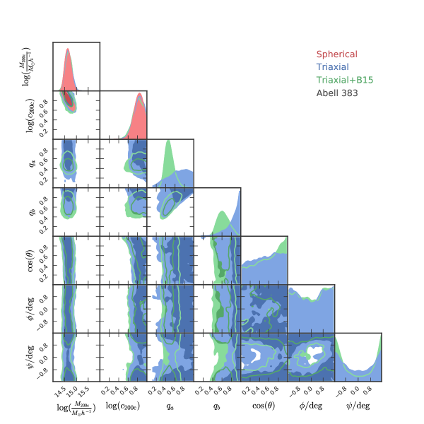
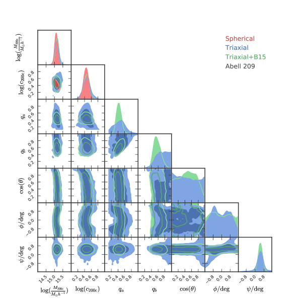
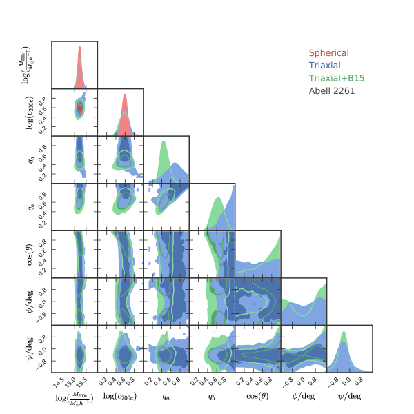
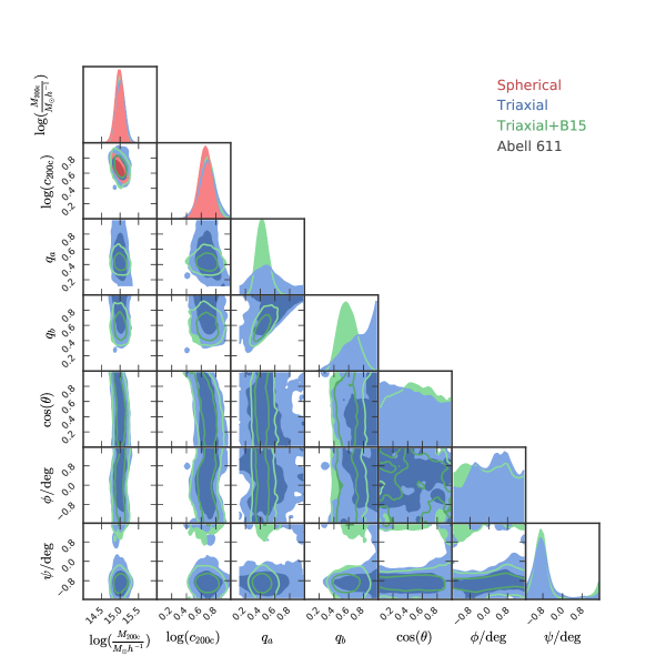
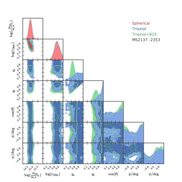
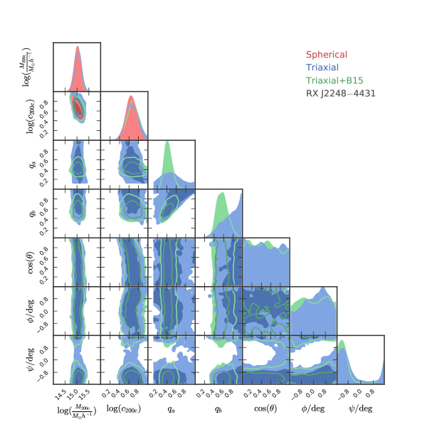
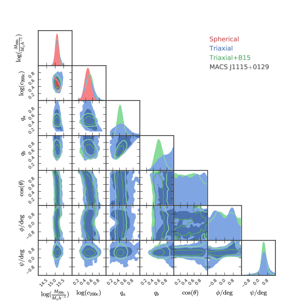
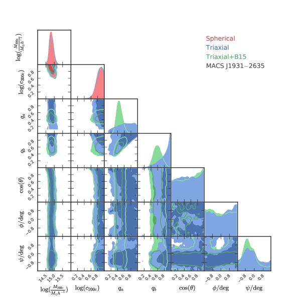
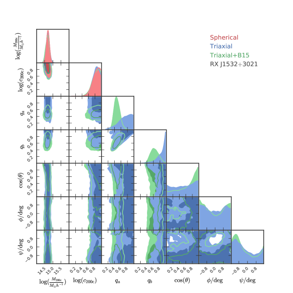
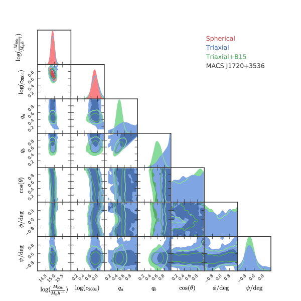
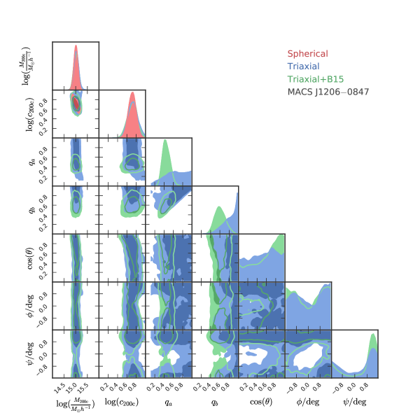
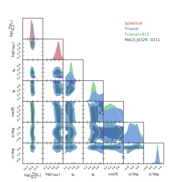
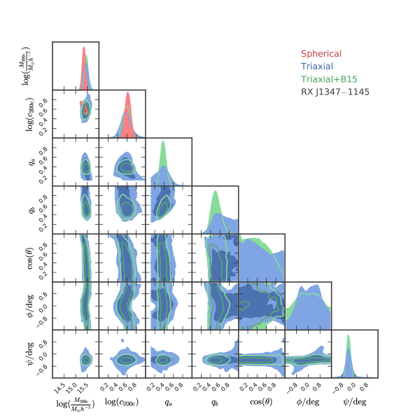
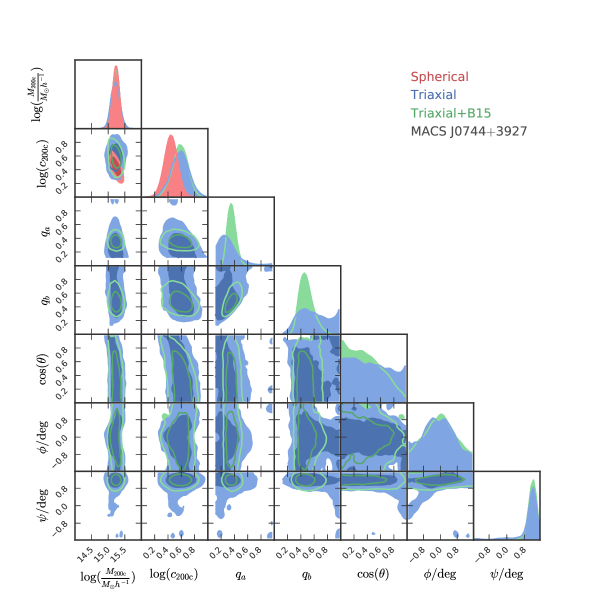
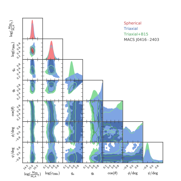
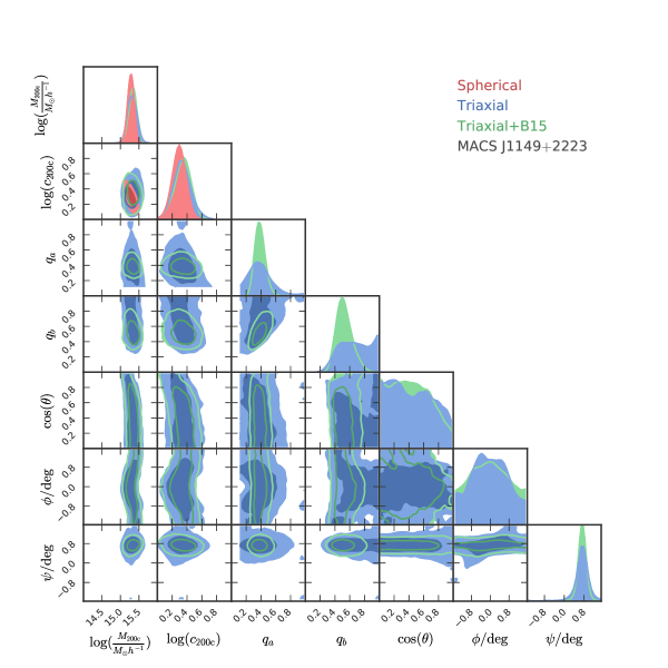
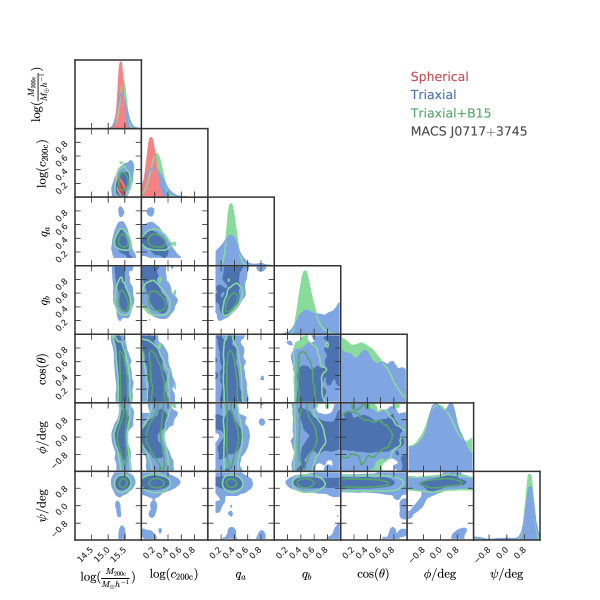
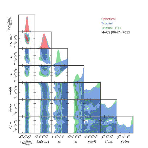
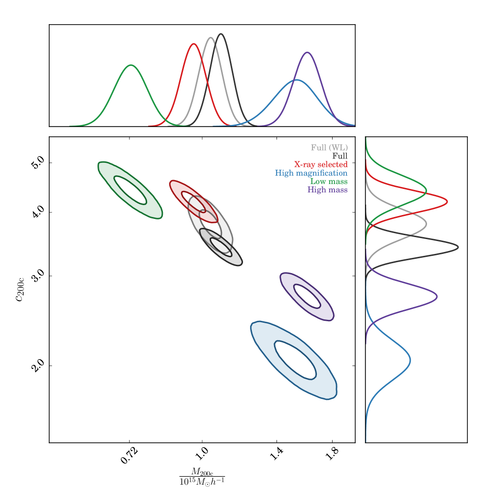
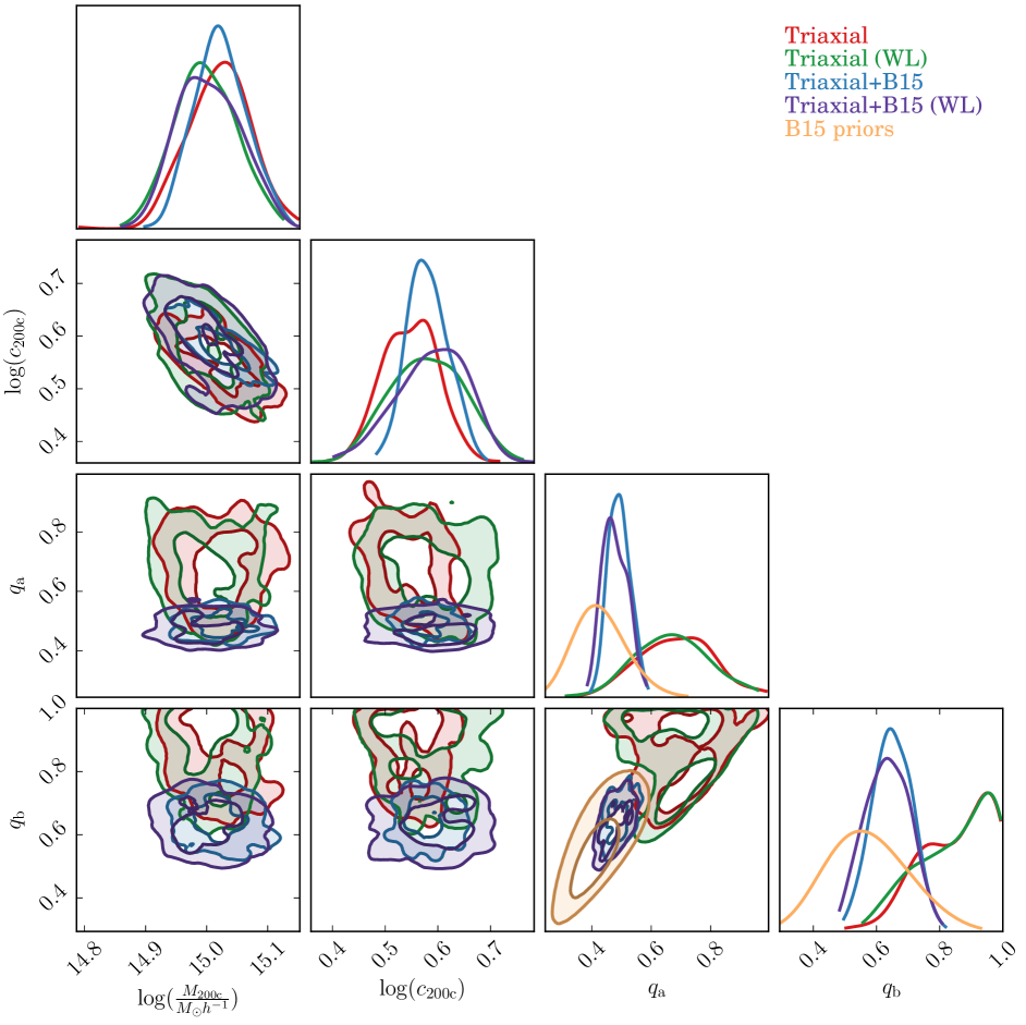
In Table 4.2 we summarize marginalized constraints on the spherical and triaxial NFW model parameters derived from the individual and ensemble modeling approaches. Here we have employed the biweight estimators of Beers et al. (1990) for the central location and scale of the marginalized posterior distributions (e.g., Sereno & Umetsu, 2011; Umetsu et al., 2014, 2015). The regression parameters of various mass scaling relations are summarized in Table 4. In Figure 1, we show the joint ensemble constraints on cluster parameters from different modeling approaches. We also show the results obatained with and without the HST lensing constraints $M_{\mathrm{SL}}(<r)$ to demonstrate the consistency between the weak and strong lensing data sets. For the results from individual cluster modeling, we show the resulting marginalized posterior distributions in Appendix A.

5.1. Consistency of Spherical Modeling

We compare our results from Spherical modeling of the 20 clusters to those of U14 and U16 for a consistency check. Both U16 and this work are based on the weak-lensing shear and magnification data obtained by U14. U16 reconstructed azimuthally averaged surface mass density profiles of these individual clusters by combining the weak-lensing data of U14 with the central HST lensing constraints $M_{\mathrm{SL}}(<r)$ from Zitrin et al. (2015).

In both U14 and U16, the NFW mass and concentration parameters were derived assuming spherical symmetry, corresponding to the case of Spherical modeling in this work. Although these three studies share the same data as input to modeling, the crucial difference of this study is that we directly fit a model profile to the 2D surface mass density maps of Umetsu et al. (2018) without azimuthal averaging. This comparison is thus useful for validating the robustness of our reconstruction and modeling procedures, for a given data set.

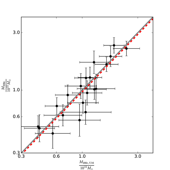
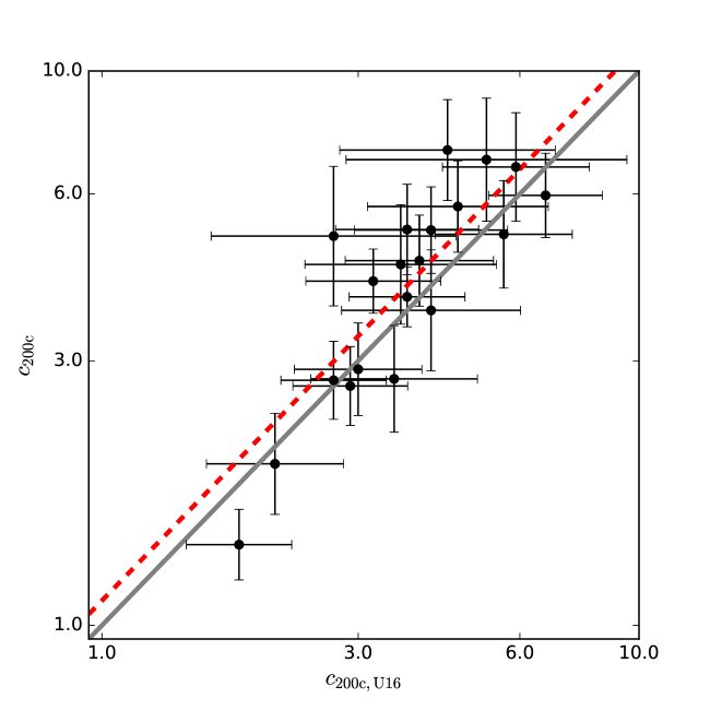
We begin with the results of individual cluster modeling. Comparing our $M_{200\mathrm{c}}$ mass estimates to those $M_{200\mathrm{c,U16}}$ from U16, we find the mean diffrence in logarithmic mass of $\left\langle\Delta\log M_{200\mathrm{c}}\right\rangle=\left\langle\log M_{200\mathrm{c}}-\log M_{200\mathrm{c,U16}}\right\rangle=-0.01\pm 0.04$, which meets the criterion of $<8\%$ (or $0.035$ dex) for consistency (see Section 3.2). Similarly, the mean difference in logarithmic concentration is $\left\langle\Delta\log c_{200\mathrm{c}}\right\rangle=\left\langle\log c_{200\mathrm{c}}-\log c_{200\mathrm{c,U16}}\right\rangle=0.04\pm 0.04.$ Except that we observe a mild increase ($0.04$ dex or $\approx 10$$\%$) in concentration with respect to U16, our results are in satisfactory agreement with U16. This comparison with U16 is shown in Figure 2.

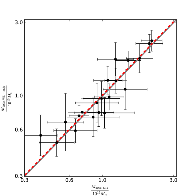
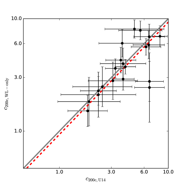
Excluding the HST lensing constraints $M_{\mathrm{SL}}(<r)$ from our Spherical modeling results in mass estimates that are consistent with those from U14 based on the one-dimensional (1D) weak-lensing analysis, with a mean difference in logarithmic mass of $\left\langle\Delta\log M_{200\mathrm{c,WL}}\right\rangle=\left\langle\log M_{200\mathrm{c,WL}}-\log M_{200\mathrm{c,U14}}\right\rangle=0.01\pm 0.04.$ This is much smaller than the systematic uncertainty in the overall mass calibration of $8\%$ (or $0.035$ dex). Similarly, the mean difference in logarithmic concentration with respect to U14 is $\left\langle\Delta c_{200\mathrm{c,WL}}\right\rangle=\left\langle\log c_{200\mathrm{c,WL}}-\log c_{200\mathrm{c,U14}}\right\rangle=-0.03\pm 0.05.$ Again, no significant tension with U14 is found, as also shown in Figure 3.

In what follows, we compare our results from joint ensemble modeling to those from U14 and U16. Since U14 and U16 constrained the $c$–$M$ relation only for the X-ray-selected subsample, we restrict our ensemble Spherical modeling to the same 16 X-ray-selected clusters for a fair comparison.

U16 constrained the NFW parameters from the stacked weak and strong lensing profile as $c_{200\mathrm{c}}=3.76^{+0.29}_{-0.27}$ and $M_{200\mathrm{c}}=\left(10.08\pm 0.7\right)\times 10^{14}\mathrm{M}_{\odot}\,h^{-1}$, respectively. In this work, joint ensemble Spherical modeling with combined weak and strong lensing yields $c_{200\mathrm{c}}=4.18^{+0.20}_{-0.19}$ and $M_{200\mathrm{c}}=\left(9.62^{+0.49}_{-0.52}\right)\times 10^{14}\mathrm{M}_{\odot}\,h^{-1}$, consistent with the 1D analysis of U16 within the quoted uncertainties. Note that this joint ensemble constraint on $c_{200\mathrm{c}}$ from our Spherical modeling is $\approx 10$$\%$ higher than that from U16 at the $1\sigma$ level. This tendency is consistent with the case of individual cluster modeling (see Figure 2). This ensemble constraint is shown in red contours in the left panel of Figure 1.

From an NFW fit to the stacked weak-lensing profile, U14 found $c_{200\mathrm{c}}=4.01^{+0.35}_{-0.32}$ and $M_{200\mathrm{c}}=\left(9.4\pm 0.70\right)\times 10^{14}\mathrm{M}_{\odot}\,h^{-1}$. Our joint ensemble Spherical modeling using the weak-lensing data alone yields $c_{200\mathrm{c}}=4.15^{+0.29}_{-0.27}$ and $M_{200\mathrm{c}}=\left(9.66^{+0.53}_{-0.51}\right)\times 10^{14}\mathrm{M}_{\odot}\,h^{-1}$, showing no significant discrepancy.

We further compare our spherical mass estimates to those fom Sereno et al. (2018). They obtained cluster masses $M_{200\mathrm{c,~{}S18}}$ from a joint analysis of weak and strong lensing, X-ray, and the SZE data sets, in both triaxial and spherical approaches. For the spherical mass comparison, we find a mean difference in logarithmic mass of $\left\langle M_{200\mathrm{c,~{}S18}}(<R)-M_{200\mathrm{c}}(<R)\right\rangle=\left(2\pm 3\right)\%$ and $\left(0\pm 1\right)\%$ at $R=1\mathrm{Mpc}\,h^{-1}$ and $1.5\mathrm{Mpc}\,h^{-1}$, respectively. This again demonstrates excellent agreement.

On the basis of these consistency tests, we find no significant tension between the results using different combinations of data sets (U14, U16, Sereno et al. (2018)), ensuring the robustness of our modeling procedures. We will discuss more results of Spherical modeling in Section 5.2.

5.2. Concentration to Mass Relations

From Bayesian regression, we determine the $c$–$M$ relation for the 16 X-ray-selected CLASH clusters as

$$c_{200\mathrm{c}}=\left(4.51\pm 0.14\right)\times\left(\frac{M_{200\mathrm{c}}}{10^{15}\mathrm{M}_{\odot}\,h^{-1}}\right)^{-0.47\pm 0.07},$$ (27)

$$c_{200\mathrm{c}}=\left(4.82\pm 0.30\right)\times\left(\frac{M_{200\mathrm{c}}}{10^{15}\mathrm{M}_{\odot}\,h^{-1}}\right)^{-0.36\pm 0.11},$$ (28)

and

$$c_{200\mathrm{c}}=\left(4.73\pm 0.28\right)\times\left(\frac{M_{200\mathrm{c}}}{10^{15}\mathrm{M}_{\odot}\,h^{-1}}\right)^{-0.36\pm 0.10},$$ (29)

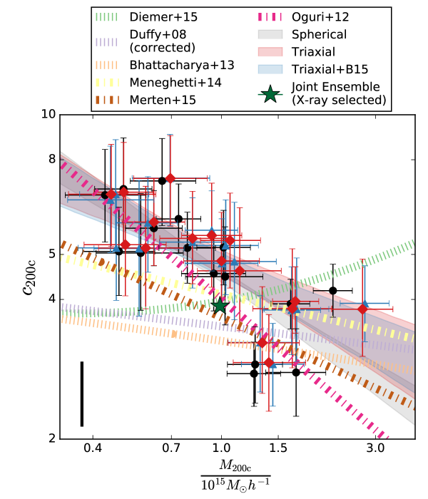
with a log-normal intrinsic scatter $D_{c_{200\mathrm{c}}}\equiv\sigma_{\log c_{200\mathrm{c}}|M_{200\mathrm{c}}}$ of $0.05$, $<0.12$ ($2\sigma$ upper bound), and $0.04$ using the Spherical, Triaxial and Triaxial+B15 modeling approaches, respectively. A redshift evolution of the NFW $c$–$M$ relation, $c\propto(1+z)^{-0.668\pm 0.341}$, was suggested for X-ray-selected CLASH-like halos in $N$-body hydrodynamical simulations (Meneghetti et al., 2014). We find that including the redshift scaling in regression analysis results in a negligible change in the inferred regression parameters within the errors. We thus ignore the redshift dependence of the $c$–$M$ relation in this study. In Figure 4, we plot the resulting scaling relations along with the individual cluster constraints for the X-ray-selected subsample. The scaling relations obtained for the full sample and the high-magnification subsample are given in Table 4.

In Figure 4, we see a steep mass dependence of the $c$–$M$ relation. Assuming spherical symmetry, we find a mass slope of $B_{c_{200\mathrm{c}}}=-0.47\pm 0.07$ for the X-ray-selected subsample, and an even steeper slope of $B_{c_{200\mathrm{c}}}=-0.65\pm 0.06$ for the full sample. Here we note that this is due in part to our fitting procedure, in which we do not account for the underlying distribution of true cluster masses. That is, the steepening of the intrinsic mass function combined with the selection function could alter the resulting distribution of true cluster masses (Sereno & Ettori, 2015). Accounting for this effect, U16 found $B_{c_{200\mathrm{c}}}=-0.44\pm 0.19$ for the same subsample, which is consistent with our results, but with a much larger uncertainty. From Triaxial modeling including additional shape and orientation parameters (with uniform priors), we find a shallower mass slope of $-0.36\pm 0.11$, which is consistent with the Spherical modeling results within the errors.

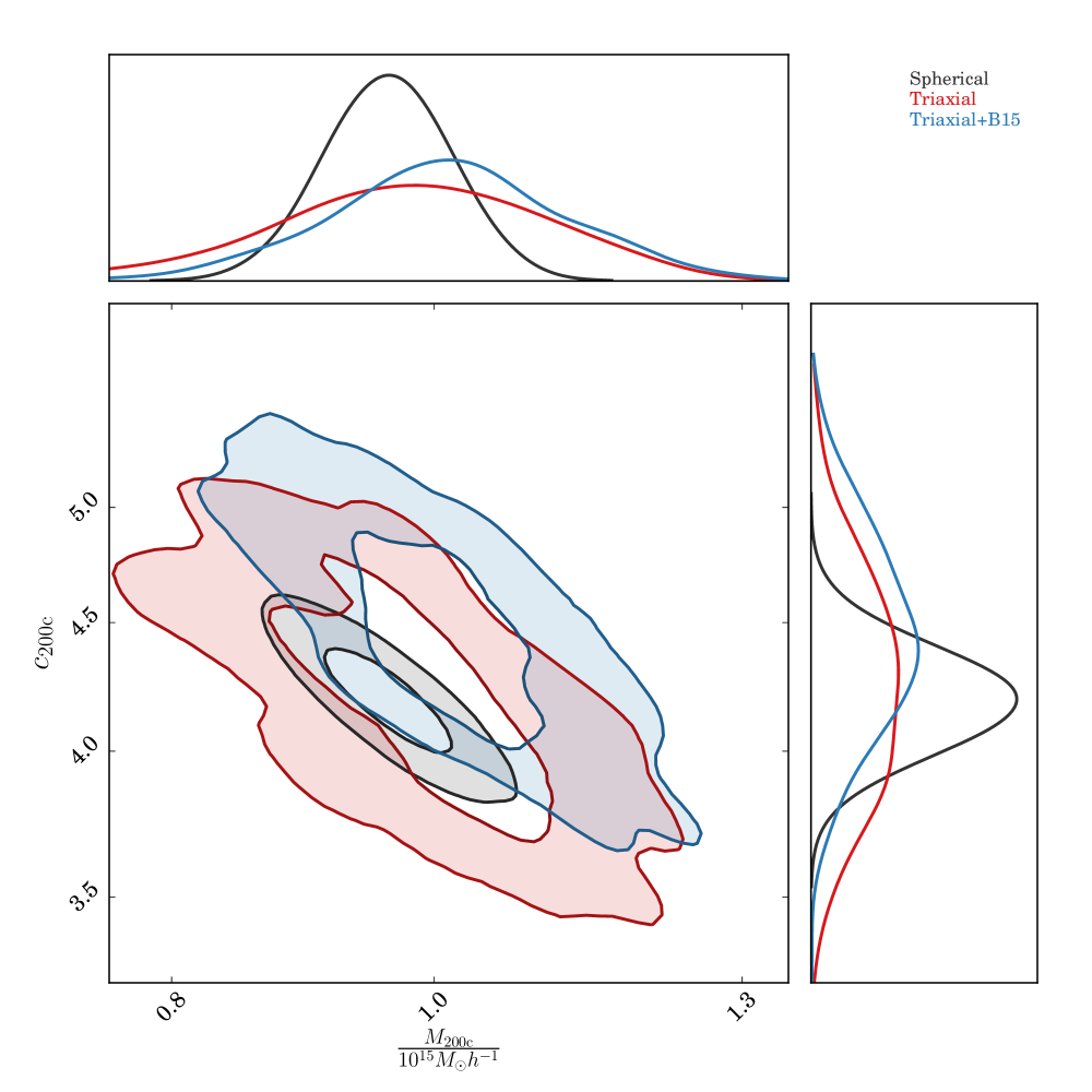
The normalization of the $c$–$M$ relation is constrained as $c_{200\mathrm{c}}=4.51\pm 0.14$ and $4.82\pm 0.30$ at the pivot mass of $M_{200\mathrm{c}}=10^{15}\mathrm{M}_{\odot}\,h^{-1}$ for Spherical and Triaxial modeling, respectively. We note that, by construction, $c_{200\mathrm{c}}(\textsf{Spherical})\leqslant c_{200\mathrm{c}}(\textsf{Triaxial})$ (see Sereno et al., 2018). On the other hand, employing the informative shape priors from B15 in Triaxial+B15 modeling does not change the results in a significant manner. Regardless of the priors chosen, the effect of triaxiality has no significant impact on the resulting $c$–$M$ relation, so that the assumption of spherical symmetry is well validated in determining the overall density structure of the CLASH clusters.

Now we discuss the results of joint ensemble modeling of the cluster mass and concentration. In the left panel of Figure 1, we show the weak-lensing-only results in gray and the weak and strong lensing results in black, both derived for the full sample of 20 clusters. Joint ensemble constraints for the X-ray-selected, high-magnification, low-mass, and high-mass subsamples are also shown in the same panel. We see a clear trend of decreasing concentration with increasing mass. In particular, the high-magnification subsample consisting of four very massive disturbed clusters ($M_{200\mathrm{c}}\approx 1.5\times 10^{15}\mathrm{M}_{\odot}\,h^{-1}$) has $c_{200\mathrm{c}}\approx 2$, much lower than other similar-mass clusters, indicating a selection effect. We will further discuss this in Section 5.2.1.

In Figure 5, we show our joint ensemble constraints on the mass and concentration parameters for the X-ray-selected subsample, obtained with three different modeling approaches (Spherical  black; Triaxial  red; Triaxial+B15  blue). In all cases, we use the weak and strong lensing constraints. From Triaxial (Triaxial+B15) modeling, we find $c_{200\mathrm{c}}=3.87^{+0.76}_{-0.11}$ and $M_{200\mathrm{c}}=\left(0.99\pm 0.11\right)\times 10^{15}\mathrm{M}_{\odot}\,h^{-1}$ ($c_{200\mathrm{c}}=4.42^{+0.41}_{-0.40}$ and $M_{200\mathrm{c}}=1.050^{+0.048}_{-0.144}\times 10^{15}\mathrm{M}_{\odot}\,h^{-1}$). Overall, triaxial modeling results in a concentration that is slightly higher than spherical modeling at the $\approx 7\%$ level, regardless of the chosen priors. As noted above, it is expected that $c_{200\mathrm{c}}(\textsf{Spherical})\leqslant c_{200\mathrm{c}}(\textsf{Triaxial})$ (Sereno et al., 2018). However, this level of difference is consistent with zero within the errors. Therefore, we conclude that the spherical symmetry is a well valid assumption in estimating the concentration of the CLASH clusters.

Figure 4.— Concentration to mass scaling relation for the 16 X-ray-selected CLASH clusters. The results of Spherical, Triaxial and Triaxial+B15 modeling are shown by black circles, red diamonds, and blue triangles, respectively. The $1\sigma$ confidence levels of the scaling relations are indicated by the shaded areas. We also plot various results from numerical simulations (Duffy et al., 2008; Bhattacharya et al., 2013; Diemer & Kravtsov, 2015) and previous observational work (Oguri et al., 2012; Meneghetti et al., 2014; Merten et al., 2015). The color codes for different authors are noted in the figure. We multiply the normalization of the $c$-$M$ relation from Duffy et al. (2008) by $1.2$ to account for the different cosmology (see the discussion in the text). The green star indicates our joint ensemble constraint from Triaxial modelling of the X-ray selected subsample. The length of the black bar at the lower-left corner indicates the level of log-normal intrinsic scatter ($D_{c_{200\mathrm{c}}}\equiv\sigma_{\log c_{200\mathrm{c}}|M_{200\mathrm{c}}}$) of $7\%$ at fixed mass, which is predicted by Meneghetti et al. (2014) for the X-ray selected sample in the CLASH survey (see the text for more details).

Figure 5.— Joint ensemble constraints on the concentration and mass for the X-ray-selected subsample of 16 CLASH clusters. The results of Spherical, Triaxial and Triaxial+B15 modeling are shown in black, red and blue, respectively.

5.2.1 Comparisons with Previous Work

We first compare our concentration to mass scaling relations to that obtained by U16. In U16, the $c$–$M$ relation for the X-ray-selected subsample is constrained as $c_{200\mathrm{c}}\propto 3.98^{+0.38}_{-0.35}\times M_{200\mathrm{c}}^{-0.44\pm 0.19}$ with a log-normal intrinsic scatter of $\sigma_{\log c_{200\mathrm{c}}|M_{200\mathrm{c}}}\approx 0.056\pm 0.026,$ assuming spherical symmetry. This is in good agreement with our Spherical modeling (see Equation (27)) at the $\lesssim 1\sigma$ level, in terms of the mass slope and intrinsic scatter. On the other hand, we find a normalization that is $\approx 13\%$ higher than U16. This trend is consistent with what we found in Section 5.1.

According to Meneghetti et al. (2014), it is expected that the mean concentration of the X-ray-selected CLASH subsample recovered from projected lensing measurements is $\approx 11\%$ higher than that for the full population of clusters. Specifically, the $c$–$M$ relation predicted for this subsample is $c_{200\mathrm{c}}\propto\left(4.1\pm 0.1\right)\times M_{200\mathrm{c}}^{-0.16\pm 0.11}$ at their median redshift of $\left\langle z\right\rangle\approx 0.35$, with an intrinsic scatter of $\sigma_{\log c_{200\mathrm{c}}|M_{200\mathrm{c}}}\approx 0.07$. The observed normalization ($A_{c_{200\mathrm{c}}}=4.51\pm 0.14$) is thus $\left(10\pm 4\right)\%$ higher than this CLASH prediction. The derived mass slope ($B_{c_{200\mathrm{c}}}=-0.47\pm 0.07$) is steeper than the CLASH prediction (Meneghetti et al., 2014) at the $2.4\sigma$ level. The predicted scatter is consistent with our measurements, but considerably smaller than the typical intrinsic scatter, $\sigma_{\log c_{200\mathrm{c}}|M_{200\mathrm{c}}}\approx 0.15$ ($\approx 0.11$), predicted for the full (relaxed) population of halos in cosmological $N$-body simulations (e.g., Duffy et al., 2008; Bhattacharya et al., 2013). This is consistent with the expectation that the X-ray-selected CLASH sample is largely ($\approx 70\%$) composed of regular and highly relaxed clusters (Meneghetti et al., 2014). The intrinsic scatter is increased by a factor of $\approx 2$ if we include the four high-magnification CLASH clusters (see Table 4).

Next, we compare our results to previous CLASH work of Merten et al. (2015), who studied 19 X-ray-selected CLASH clusters. They simultaneously combined HST strong+weak lensing constraints (specifically, HST shear catalogs plus locations and redshifts of multiple images) with wide-field shear catalogs of Umetsu et al. (2014) to reconstruct 2D mass maps of individual clusters. Weak magnification lensing was not used in their analysis. Cluster mass estimates were obtained from spherical NFW fits to azimuthally averaged surface mass density profiles. Assuming spherical symmetry, Merten et al. (2015) found $c_{200\mathrm{c}}\propto\left(3.66\pm 0.16\right)\times M_{200\mathrm{c}}^{-0.32\pm 0.18},$ with a log-normal intrinsic scatter of $0.07$, in good agreement with our results in terms of the mass slope and intrinsic scatter. However, the normalization obtained by Merten et al. (2015) is significantly lower than our results, likely arising from the different reconstruction methods.

We then compare our results to those of Sereno et al. (2017a), who carried out a 1D weak-lensing analysis to derive the $c$–$M$ relation for SZE-selected clusters from the Planck survey. Examining their $c$–$M$ relation with $M_{200\mathrm{c}}=10^{15}\mathrm{M}_{\odot}\,h^{-1}$ and the median redshift of our full sample, $\left\langle z_{\mathrm{d}}\right\rangle=0.377$, we find $c_{200\mathrm{c}}=4.04^{+6.59}_{-2.50},$ which is consistent with our Spherical modeling results for our full sample within large errors.

In addition, we compare our results to Oguri et al. (2012), who combined strong and weak lensing constraints in a 1D analysis to derive the $c$–$M$ relation for a sample of 28 strong-lensing-selected clusters from the Sloan Digital Sky Survey. The best-fit $c$–$M$ relation of Oguri et al. (2012) is $c_{\mathrm{vir}}=\left(7.7\pm 0.6\right)\times\left(M_{\mathrm{vir}}/5\times 10^{14}\mathrm{M}_{\odot}\,h^{-1}\right)^{-0.59\pm 0.12},$ with a log-normal intrinsic scatter of $\sigma_{\log c_{200\mathrm{c}}|M_{200\mathrm{c}}}=0.12$ defined with the virial overdensity. We convert this relation to that with $\Delta=200$ by substituting $M_{200\mathrm{c}}=0.88M_{\mathrm{vir}}$ and $c_{200\mathrm{c}}=0.83C_{\mathrm{vir}}$ at $M_{\mathrm{vir}}=5\times 10^{14}\mathrm{M}_{\odot}\,h^{-1}$ and the median redshift of our full sample, $\left\langle z_{\mathrm{d}}\right\rangle=0.377$. The resulting relation using a pivot mass of $10^{15}\mathrm{M}_{\odot}\,h^{-1}$ is $c_{200\mathrm{c}}=\left(4.0\pm 0.3\right)\times\left(M_{200\mathrm{c}}/10^{15}\mathrm{M}_{\odot}\,h^{-1}\right)^{-0.59\pm 0.12},$ in good agreement with our full-sample results (Table 4).

This comparison is particularly interesting because the Oguri et al. (2012) sample was selected by the presence of strong-lensing features, specifically giant arcs. In contrast, the high-magnification CLASH clusters were selected by their high lensing magnification properties, with the goal of searching for strongly lensed galaxies at high redshifts. The giant-arc selection of Oguri et al. (2012) preferentially selects clusters that are more centrally concentrated and/or elongated along the line of sight, resulting in a positive bias in the apparent degree of concentration relative to the full population of clusters. Importantly, this bias is predicted to be mass dependent and more prominent for low mass clusters (Oguri et al., 2012, e.g., estimated concentration being biased high by $\approx 80\%$ for $M_{\mathrm{vir}}\approx 8\times 10^{13}\mathrm{M}_{\odot}\,h^{-1}$ and $\lesssim 20\%$ for $M_{\mathrm{vir}}\gtrsim 10^{15}\mathrm{M}_{\odot}\,h^{-1}$). In this work, we find an opposite trend of significantly lower concentration for high-magnification-selected clusters (Tables 4.2 and 4). This is expected for typical merging, high-mass clusters, where the mass distribution is not as concentrated as relaxed systems. In fact, our high-magnification clusters are found to be dynamically disturbed systems (Zitrin et al., 2013; Medezinski et al., 2013; Balestra et al., 2016; Jauzac et al., 2017), where complex merging events are taking place. Nevertheless, this comparison suggests that clusters selected by their strong-lensing features tend to be a highly biased population in terms of their morphology and dynamical state.

Finally, we compare our joint ensemble constraints (Table 4.2) to recent simulation work of Duffy et al. (2008), Bhattacharya et al. (2013), and Diemer & Kravtsov (2015). Here we compare their predictions to our results from Spherical modeling because they measured halo mass and concentration from spherically averaged density profiles of simulated halos. Overall, our conclusions are not altered significantly if comparing to our triaxial results, given the good agreement between the spherical and triaxial results, regardless of the priors chosen.

Duffy et al. (2008) characterized the $c$–$M$ relation for both relaxed and full populations of simulated halos at $z\lesssim 2$ in the WMAP5 cosmology ($\Omega_{\mathrm{m}}=0.258$ and $H_{0}=0.719$). The mean concentration predicted for the full (relaxed) population of halos is $c_{200\mathrm{c}}\approx 2.91$ ($\approx 3.30$) at $M_{200\mathrm{c}}=10^{15}\mathrm{M}_{\odot}\,h^{-1}$ and $z_{\mathrm{d}}=0.377$, which is lower than $c_{200\mathrm{c}}=3.42^{+0.14}_{-0.15}$ ($4.18^{+0.20}_{-0.19}$) by $15\%$ ($21\%$) obtained for our full (X-ray-selected) sample. This is in line with the finding of Dutton & Macciò (2014) that the WMAP5 cosmology assumed in Duffy et al. (2008) yields a concentration that is lower by $\approx 20\%$ relative to the Planck cosmology. Bhattacharya et al. (2013) modeled the halo concentration as a function of the halo peak height. Their model yields $c_{200\mathrm{c}}=3.59$ and $3.71$ at $M_{200\mathrm{c}}=10^{15}\mathrm{M}_{\odot}\,h^{-1}$ for their full and relaxed samples, respectively, with an intrinsic scatter of $\approx 0.33$. Our result for the full sample ($c_{200\mathrm{c}}=3.42^{+0.14}_{-0.15}$) is in good agreement with their prediction. Given the scatter and measurement uncertainty, these values are not in severe tension with what we measured in this work.

We then compare our results to the model of Diemer & Kravtsov (2015), who also characterized the halo concentration as a function of the halo peak height. Their model yields $c_{200\mathrm{c}}=3.73$ for the typical mass of our sample, $M_{200\mathrm{c}}\approx 10^{15}\mathrm{M}_{\odot}\,h^{-1}$, which shows no tension with our measurement (black contours in the left panel of Figure 1).

The comparisons we discussed above can be visualized in Figure 4. To sum up, our results on the $c$–$M$ relation are in satisfactory agreement with previous lensing studies. A better agreement can be achieved once the selection function, the cosmology adopted, and/or the modeling systematics are taken into account. We find that the typical values of halo concentration ($A_{c_{200\mathrm{c}}}$) range from $c_{200\mathrm{c}}\approx 3$ to $\approx 4.5$ at $M_{200\mathrm{c}}=10^{15}\mathrm{M}_{\odot}\,h^{-1}$, largely depending on the sample selection rather than the modeling assumption on the shape of clusters.

Figure 6.— Minor-to-major axis ratio to mass scaling relation for our cluster sample. The results of Triaxial and Triaxial+B15 modeling are shown by red diamonds and blue triangles, respectively. The 16 X-ray-selected (4 high-magnification) CLASH clusters are indicated by filled (open) markers. The best-fit scaling relations and their $1\sigma$ confidence regions are shown by shaded areas.

Figure 7.— Marginalized posterior distributions of the intrinsic axis ratios $q_{\mathrm{a}}$ and $q_{\mathrm{b}}$ derived from joint ensemble modeling of our full sample of 20 clusters. The results of the Triaxial and Triaxial+B15 modeling are shown in red and blue, respectively. The B15 prior distribution evaluated at the typical mass $M_{200\mathrm{c}}=10^{15}\mathrm{M}_{\odot}\,h^{-1}$ and the median redshift $\left\langle z_{\mathrm{d}}\right\rangle=0.377$ is shown in yellow.

5.3. Axis Ratio to Mass Relations

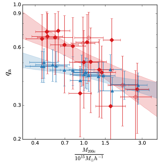
Here we present the minor-to-major axis ratio to mass scaling relation for our full sample of 20 clusters derived using the Triaxial and Triaxial+B15 modeling approaches (Equations (30) and (31)):

$$q_{\mathrm{a}}=\left(0.52\pm 0.04\right)\times\left(\frac{M_{200\mathrm{c}}}{10^{15}\mathrm{M}_{\odot}\,h^{-1}}\right)^{-0.36\pm 0.13},$$ (30)

and

$$q_{\mathrm{a}}=\left(0.44\pm 0.02\right)\times\left(\frac{M_{200\mathrm{c}}}{10^{15}\mathrm{M}_{\odot}\,h^{-1}}\right)^{-0.14\pm 0.07},$$ (31)

with an intrinsic scatter $D_{q_{\mathrm{a}}|M_{200\mathrm{c}}}$ of $0.05$ and $<~{}0.06~{}(2\sigma~{}\mathrm{upper~{}bound})$, respectively.

We plot these results in Figure 6 in a similar manner as in Figure 4. There is no clear difference in the resulting $q_{\mathrm{a}}$–$M$ relations between the X-ray-selected and high-magnification subsamples. We thus focus on the results based on the full sample hereafter. We see from Figure 6 that in Triaxial modeling, the errors of $q_{\mathrm{a}}$ for individual clusters are considerably large. However, the statistical ensemble behavior shows that $q_{\mathrm{a}}\approx\left(0.52\pm 0.04\right)$ at $M_{200\mathrm{c}}=10^{15}\mathrm{M}_{\odot}\,h^{-1}$ and it scales as $q_{\mathrm{a}}\propto M_{200\mathrm{c}}^{-0.36\pm 0.13}$ at the $2.7\sigma$ level, indicating that more massive clusters tend to be less spherical. On the other hand, introducing informative shape priors in Triaxial+B15 modeling yields an ensemble average of $q_{\mathrm{a}}\approx\left(0.44\pm 0.02\right)$ at the pivot mass $M_{200\mathrm{c}}=10^{15}\mathrm{M}_{\odot}\,h^{-1}$ and a shallower slope of $B_{q_{\mathrm{a}}}\approx\left(-0.14\pm 0.07\right)$. This corresponds to a marginal shfit in $A_{q_{\mathrm{a}}}$ and $B_{q_{\mathrm{a}}}$ at the $2\sigma$ and $1.3\sigma$ levels, respectively, with respect to the case using uniform priors. On the basis of the results above, we have detected a non-spherical shape of the clusters. The average minor-to-major axis ratio $q_{\mathrm{a}}$ is $\approx 0.5$, depending on the priors used, and it monotonically decreases with increasing cluster mass at the $\lesssim 2.7\sigma$ level.

In Figure 1, we show joint ensemble constraints on the concentration, mass, and axis ratios for the full sample obtained with different modeling approaches and data sets. It is seen in the right panel of Figure 1 that there is no clear correlation between the shape parameters (i.e., axis ratios) and the overall structural parameters (i.e., concentration and mass) regardless of the priors. This is consistent with the implication in Section 5.2 that the assumption of cluster shapes does not statistically affect the $c$–$M$ relation of the CLASH clusters. We see from the right panel of Figure 1 that including the HST lensing data $M_{\mathrm{SL}}(<r)$ results in a lower concentration, but it does not alter the axis ratios. Conversely, introducing the informative shape priors from B15 has an impact on the axis ratios, but not on the mass and concentration parameters.

Figure 8.— Comparison between the observational constraints on $q_{\mathrm{a}}$ and the theoretical predictions of Despali et al. (2014), B15, Suto et al. (2016), and Vega-Ferrero et al. (2017) evaluated at the median redshift of $\left\langle z_{\mathrm{d}}\right\rangle=0.377$. The shaded regions indicate the intrinsic scatter of $q_{\mathrm{a}}$ at fixed halo mass predicted by the respective theoretical models.

Figure 9.— Marginalized posterior distributions of the intrinsic axis ratios $q_{\mathrm{a}}$ and $q_{\mathrm{b}}$ derived from joint ensemble modeling of the low-mass and high-mass subsamples. The results of the Triaxial and Triaxial+B15 modeling for the low (high) mass subsample are shown in red and yellow (black and gray), respectively.

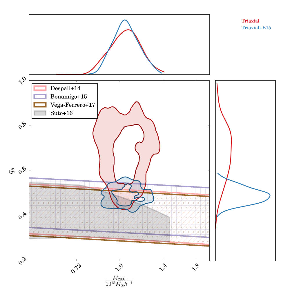
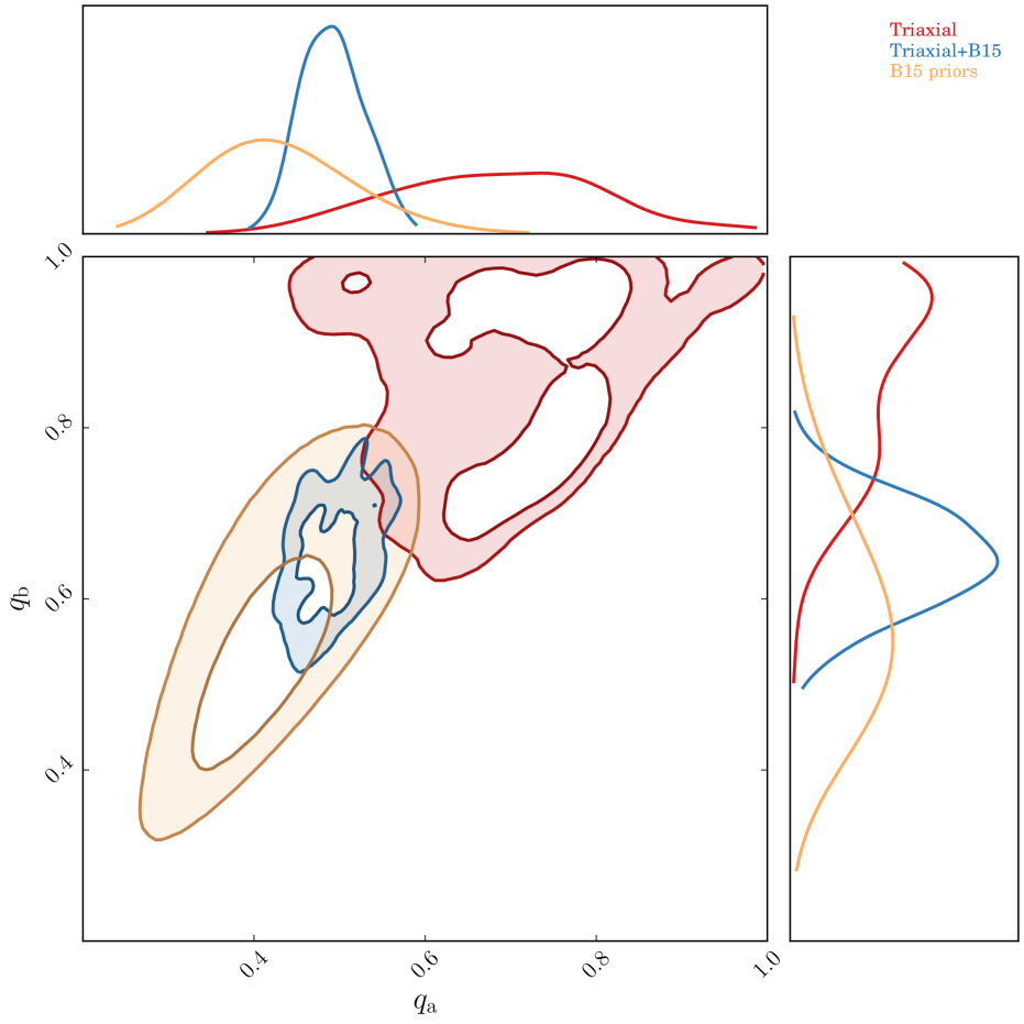
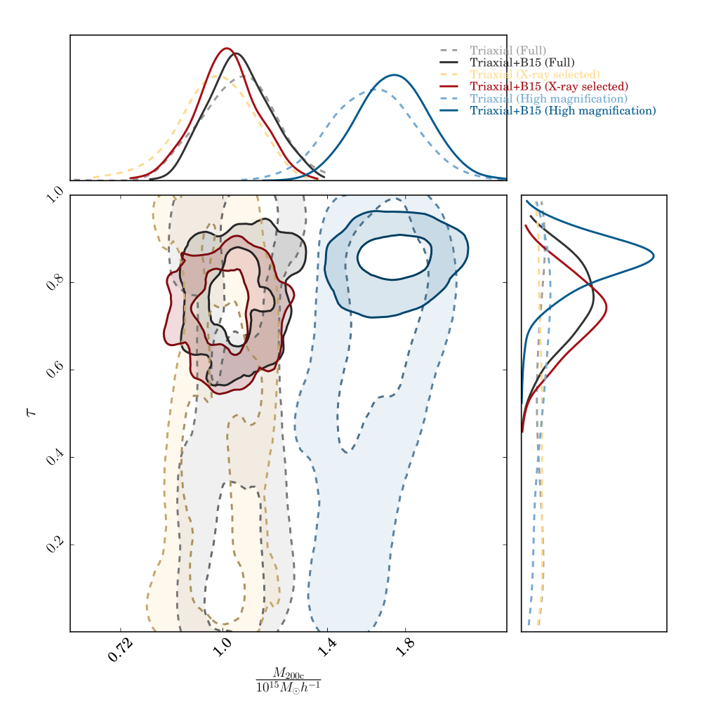
We show in Figure 7 our joint ensemble constraints on the intrinsic shape parameters for our full sample of 20 clusters, along with the B15 prior distribution. We constrain the minor-to-major axis ratio as $q_{\mathrm{a}}=0.652^{+0.162}_{-0.078}$ using uniform priors, which is higher than the expectation from the B15 prior distribution, $q_{\mathrm{a}}=0.412^{+0.095}_{-0.083}$, at the $\lesssim 1.5\sigma$ level. Employing the B15 priors in Triaxial+B15 modeling yields $q_{\mathrm{a}}=0.499^{+0.018}_{-0.056}$, which is consistent with the Triaxial constraint at the $\lesssim 1\sigma$ level, given the long tail of the posterior distribution.

Furthermore, we compare in Figure 8 our joint ensemble constraints on $q_{\mathrm{a}}$ for the full sample with theoretical predictions from $N$-body numerical simulations of Despali et al. (2014), B15, Suto et al. (2016), and Vega-Ferrero et al. (2017). Note that we evaluate the theoretical predictions in Figure 8 at the median redshift of our cluster sample, $\left\langle z_{\mathrm{d}}\right\rangle=0.377$. We see that our constraints on $q_{\mathrm{a}}$ obtained using uniform priors are in favor of the axis ratio that is higher than the theoretical predictions. However, this trend is only at the $\lesssim 1.5\sigma$ level and not statistically significant. It is worth mentioning that including baryonic physics in numerical simulations results in a rounder shape of galaxy clusters (Kazantzidis et al., 2004; Bryan et al., 2013; Suto et al., 2017), which better agrees with our results based on the uniform priors than the purely $N$-body simulations. With upcoming large cluster surveys to dramatically improve statistics, this work demonstrates an opportunity to constrain the effects of baryonic feedback on the halo shape by using gravitational lensing.

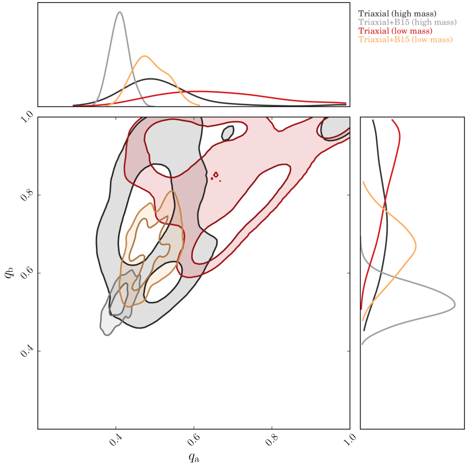
Conversely, we do not have informative constraints on the second axis ratio $q_{\mathrm{b}}$ in Triaxial modeling with uniform priors (see Table 4.2 and the right panel of Figure 1): We can only constrain the lower bound of $q_{\mathrm{b}}$ for the full sample as $0.73$, $0.63$ and $0.50$ at the $1\sigma$, $2\sigma$ and $3\sigma$ levels, respectively. Introducing the B15 priors in Triaxial+B15 modeling gives $q_{\mathrm{b}}=0.636^{+0.078}_{-0.045}$, compared to the expectation from the B15 prior distribution, $q_{\mathrm{b}}=0.55^{+0.14}_{-0.11}$. Taking the covariance between $q_{\mathrm{a}}$ and $q_{\mathrm{b}}$ into account, the overall discrepancy between our lensing data and the B15 priors is at the $\lesssim 2.5\sigma$ level. Therefore, we do not have statistically significant evidence for a strong tension between the lensing data and the B15 simulations.

Additionally, we show in Figure 9 joint ensemble constraints on the axis ratios for the low-mass and high-mass subsamples. We observe that (1) the discrepancy between the Triaxial modeling and Triaxial+B15 modeling is smaller for the high mass samples, and (2) the constraints are significantly stronger for the high mass sample, suggesting that the weak constraints on the shape parameters for the full sample are likely due to the inclusion of the low mass clusters.

We note that we currently do not have compelling constraints on the intrinsic shape (especially $q_{\mathrm{b}}$) of clusters based on the lensing data alone (using uninformative uniform priors). Nevertheless, we observe a marginal discrepancy between the lensing data and simulations, which can be better examined with a large statistical sample of clusters.

5.4. Geometrical Factor to Mass Relations

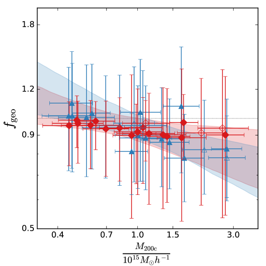
We constrain the geometrical factor to mass scaling relation for our full sample of 20 clusters from Triaxial and Triaxial+B15 modeling as

$$f_{\mathrm{geo}}=\left(0.93\pm 0.07\right)\times\left(\frac{M_{200\mathrm{c}}}{10^{15}\mathrm{M}_{\odot}\,h^{-1}}\right)^{-0.14\pm 0.15},$$ (32)

and

$$f_{\mathrm{geo}}=\left(0.96\pm 0.07\right)\times\left(\frac{M_{200\mathrm{c}}}{10^{15}\mathrm{M}_{\odot}\,h^{-1}}\right)^{-0.21\pm 0.12},$$ (33)

with an intrinsic scatter $D_{f_{\mathrm{geo}}|M_{200\mathrm{c}}}$ of $<~{}0.34~{}(2\sigma~{}\mathrm{upper~{}bound})$ and $<~{}0.26~{}(2\sigma~{}\mathrm{upper~{}bound})$, respectively. The geometrical factor $f_{\mathrm{geo}}$ is a derived quantity from the posterior distributions of the triaxial NFW parameters according to Equation (16). Specifically, $f_{\mathrm{geo}}$ is defined as the ratio of the line-of-sight half length of a triaxial ellipsoid to the geometric-mean scale-radius of its isodensity contour projected on the sky. Therefore, it represents the degree of line-of-sight elongation of the mass distribution. A geometrical factor greater (smaller) than unity indicates a line-of-sight excess (deficit) of mass structure.

We show the results of the geometrical factor to mass scaling relations in Figure 10. Although the geometrical factor is a very noisy quantity for individual clusters, the ensemble behavior from the best-fit scaling relations suggests no significant deviation from random orientations (i.e., $f_{\mathrm{geo}}$ is consistent with unity within the quoted $1\sigma$ uncertainties) regardless of the shape priors (uniform or B15). We find no significant evidence of a dependence of $f_{\mathrm{geo}}$ on cluster mass. A mild trend at the $\lesssim 2\sigma$ level is found when the B15 priors are employed.

We stress that, given the fact that lensing can only probe the integrated mass along the line of sight, we do not have a sensitivity to the line-of-sight elongation of clusters using lensing data alone (Dietrich et al., 2014). Hence, we must rely on external information (e.g., X-ray/SZE data or simulation priors) to better constrain the orientation of clusters. With the B15 priors applied on the axis ratios, we extract the biweight center location of the marginalized posterior distribution of $\cos(\theta)$ for each cluster (Section 5). The distribution of $\cos(\theta)$ spans a wide range between $0.37$ and $0.70$, with a median value of $\left\langle\cos(\theta)\right\rangle=0.55$ and a typical biweight scale of $\approx 0.30$. This corresponds to a mean inclining angle of $\cos^{-1}\left(\left\langle\cos(\theta)\right\rangle\right)\approx 57\deg$, suggesting that the orientations of our sample are nearly random (i.e., no orientation bias). This is consistent with our results on the $f_{\mathrm{geo}}$–$M$ relation (Table 4) regardless of the chosen sample, and in line with the theoretical expectation for the X-ray-selected CLASH clusters (Meneghetti et al., 2014). It is worth mentioning that a positive bias at a level of $3\%$–$6\%$ was suggested in the mass estimates of stacked weak-lensing measurements for optically selected clusters (Dietrich et al., 2014), while there is no clear indication of orientation bias for our clusters that are largely selected by their X-ray properties.

Figure 10.— Geometrical factor ($f_{\mathrm{geo}}$) to mass scaling relation. The results of Triaxial and Triaxial+B15 modeling are shown by red diamonds and blue triangles, respectively. The 16 X-ray-selected (4 high-magnification) CLASH clusters are indicated by filled (open) markers. The best-fit scaling relations and their $1\sigma$ confidence regions are shown by shaded areas. The gray thin line indicates $f_{\mathrm{geo}}=1$.

5.5. Triaxiality to Mass Relations

The degree of triaxiality $\mathcal{T}$ is a quantity derived from the posterior distributions of the intrinsic axis ratios (Equation (17)). A prolate mass distribution (i.e., $q_{\mathrm{a}}=q_{\mathrm{b}}$) has $\mathcal{T}=1$, while a oblate shape (i.e., $q_{\mathrm{a}}<q_{\mathrm{b}}=1$) has $\mathcal{T}=0$.

We stress again that we can only constrain the lower bound of the second axis ratio $q_{\mathrm{b}}$ and thus the upper bound on the degree of triaxiality $\mathcal{T}$ from Triaxial modeling when using uniform priors. Accordingly, we only present the $2\sigma$ upper bound for the results from Triaxial modeling. The $2\sigma$ upper bound on the $\mathcal{T}$–$M$ relation from Triaxial modeling is

$$\mathcal{T}<0.69\times\left(\frac{M_{200\mathrm{c}}}{10^{15}\mathrm{M}_{\odot}\,h^{-1}}\right)^{0.07\pm 0.19},$$ (34)

while the best-fit $\mathcal{T}$–$M$ relation from Triaxial+B15 modeling is

$$\mathcal{T}=\left(0.79\pm 0.03\right)\times\left(\frac{M_{200\mathrm{c}}}{10^{15}\mathrm{M}_{\odot}\,h^{-1}}\right)^{0.06\pm 0.07},$$ (35)

with an intrinsic scatter of $<~{}0.13~{}(2\sigma~{}\mathrm{upper~{}bound})$. We show the results of the $\mathcal{T}$–$M$ relation as well as the individual cluster constraints in Figure 11.

Figure 11.— Triaxiality to mass scaling relation. The results of Triaxial and Triaxial+B15 modeling are shown by red diamonds and blue triangles, respectively. The 16 X-ray-selected (4 high-magnification) CLASH clusters are indicated by filled (open) markers. The $1\sigma$ confidence region of the Triaxial+B15 modeling is shown by the blue shaded area. The $2\sigma$ upper bound of the scaling relation from the Triaxial modeling is indicated by the red shaded area.

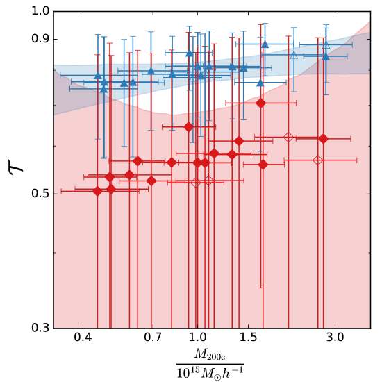
In Figure 11, a clear offset in the normalization $A_{\mathcal{T}}$ is seen between the Triaxial and Triaxial+B15 modeling results: The degree of triaxiality is constrained as $\mathcal{T}\approx 0.79\pm 0.03$ at the pivot mass $M_{200\mathrm{c}}=10^{15}\mathrm{M}_{\odot}\,h^{-1}$ using the B15 priors, and the offset in the normalization relative to the Triaxial results is at the $\approx 3\sigma$ level. This discrepancy is strongly driven by the fact that we can only constrain the lower bound of the intermediate-to-major axis ratio $q_{\mathrm{b}}$ from Triaxial modeling, resulting in a nearly flat distribution of $\mathcal{T}$. This can be further seen in Figure 12, where we plot $\mathcal{T}$ against cluster mass using the posteriors joint ensemble modeling (full, X-ray-selected, and high-magnification samples). Without the B15 priors, $\mathcal{T}$ is essentially unconstrained by the lensing data alone. On the other hand, employing the B15 priors gives $\mathcal{T}\approx 0.8$, implying a prolate configuration of the CLASH clusters. We find that the posterior constraints on the mass slope are not sensitive to the chosen prior ($B_{\mathcal{T}}\approx 0.07$), although the uncertainties are too large to claim a significant mass dependence. Even though the CLASH clusters exhibit non-spherical shapes, we echo that spherical symmetry is a well-validated assumption in estimating the cluster mass and concentration (see Section 5.2).

Figure 12.— Constraints on the degree of triaxiality $\mathcal{T}$ and cluster mass $M_{200\mathrm{c}}$ from joint ensemble modeling of different cluster subsamples. Using uninformative uniform priors, the constraints on $\mathcal{T}$ from Triaxial modeling are shown in gray (yellow, light blue) for the full (X-ray selected, high-magnification) sample. Using the B15 priors, the constraints on $\mathcal{T}$ are shown in black (red, dark blue) for the full (X-ray selected, high-magnification) sample.

6. Conclusions

In this paper, we have combined the wide-field weak-lensing mass maps obtained by Umetsu et al. (2018) with the central CLASH-HST lensing constraints (Zitrin et al., 2015; Umetsu et al., 2016) to perform three-dimensional modeling of the intrinsic mass distribution for a sample of 16 X-ray-selected and 4 high-magnification clusters targeted by the CLASH survey. These clusters span a mass range of $4\times 10^{14}\mathrm{M}_{\odot}\,h^{-1}\lesssim M_{200\mathrm{c}}<20\times 10^{14}\mathrm{M}_{\odot}\,h^{-1}$ and a redshift range of $0.18<z<0.7$, with a median redshift of $\approx 0.377$. Specifically, we have forward-modeled these lensing data sets assuming a triaxial NFW halo in a Bayesian framework, and constrained the mass $M_{200\mathrm{c}}$, concentration $c_{200\mathrm{c}}$, intrinsic axis ratios (minor-to-major ratio $q_{\mathrm{a}}$ and intermediate-to-major ratio $q_{\mathrm{b}}$), and orientation angles. For the case of triaxial modeling, we considered either uniform priors on all parameters or, alternatively, informative shape priors on $q_{\mathrm{a}}$ and $q_{\mathrm{b}}$ taken from cosmological $N$-bod simulations (Bonamigo et al., 2015). We have also performed spherical NFW modeling with the $M_{200\mathrm{c}}$ and $c_{200\mathrm{c}}$ parameters, while fixing the other parameters to the spherical configuration. We performed Bayesian modeling of both individual and ensemble clusters using the combined weak and strong lensing data sets. With the observed constraints on each individual cluster, we have investigated mass-scaling relations of the halo concentration $c_{200\mathrm{c}}$, the minor-to-major axis ratio $q_{\mathrm{a}}$, the geometrical factor $f_{\mathrm{geo}}$, and the degree of triaxiality $\mathcal{T}$.

Our results show that the halo concentration decreases with increasing mass, as found by previous work assuming spherical symmetry. The results are insensitive to both the assumed cluster geometry (spherical or triaxial) and the chosen shape prior. However, we find that the selection of clusters plays an important role. The four high-magnification CLASH clusters ($M_{200\mathrm{c}}\approx 1.5\times 10^{15}\mathrm{M}_{\odot}\,h^{-1}$) have a significantly low concentration, compared to the X-ray-selected CLASH subsample. For the 16 X-ray-selected CLASH clusters, we find a mean concentration of $c_{200\mathrm{c}}=4.82\pm 0.30$ at the pivot mass $M_{200\mathrm{c}}=10^{15}\mathrm{M}_{\odot}\,h^{-1}$, and it scales as $M_{200\mathrm{c}}^{-0.36\pm 0.11}$ according to triaxial modeling with uniform priors. On the other hand, jointly modeling this subsample assuming a triaxial NFW halo, we obtain joint ensemble constraints of $c_{200\mathrm{c}}=3.87^{+0.76}_{-0.11}$ and $M_{200\mathrm{c}}=\left(0.99\pm 0.11\right)\times 10^{15}\mathrm{M}_{\odot}\,h^{-1}$. Our results are consistent with previous work from observations and simulations. A better agreement can be achieved if accounting for the sample selection, geometry of clusters, the background cosmology adopted, and the choice of the priors. The results from triaxial modeling are in good agreement with those from spherical modeling within the errors, suggesting that the assumption of spherical symmetry is well validated in estimating the overall mass profile of the CLASH clusters, even though we do observe evidence of aspherical shapes of clusters.

When using uninformative uniform priors, we obtain joint ensemble constraints on the minor-to-major axis ratio of $q_{\mathrm{a}}=0.652^{+0.162}_{-0.078}$ at the typical mass $M_{200\mathrm{c}}=10^{15}\mathrm{M}_{\odot}\,h^{-1}$ for our full sample of 20 CLASH clusters. Conversely, only a lower bound on the intermediate-to-major axis ratio $q_{\mathrm{b}}$ is obtained as $q_{\mathrm{b}}>0.632$ at the $2\sigma$ level. Using the B15 priors gives improved joint ensemble constraints of $q_{\mathrm{a}}=0.499^{+0.018}_{-0.056}$ and $q_{\mathrm{b}}=0.636^{+0.078}_{-0.045}$, respectively. The resulting $q_{\mathrm{a}}$–$M$ relation suggests that $q_{\mathrm{a}}$ decreases with increasing halo mass as $M_{200\mathrm{c}}^{-0.36\pm 0.13}$ and $M_{200\mathrm{c}}^{-0.14\pm 0.07}$ based on the results with the uniform and B15 priors, respectively. Overall, no significant tension is seen between the lensing data and the numerical predictions from B15 in terms of the intrinsic cluster axis ratios. Our results suggest that we currently do not have strong constraints ($\lesssim 3\sigma$) on the intrinsic shape of clusters based on gravitational lensing alone, unless informative shape priors are employed.

We have also studied the geometrical factor $f_{\mathrm{geo}}$, an indicator of the line-of-sight elongation of cluster mass distributions. We find that our sample shows no significant deviation from isotropic, random orientations: $f_{\mathrm{geo}}=0.93\pm 0.07$ and $f_{\mathrm{geo}}=0.96\pm 0.07$ based on the uniform and B15 priors, respectively. The results are in agreement with the theoretical expectation for the CLASH clusters dominated by relaxed systems (Meneghetti et al., 2014). No significant mass dependence of $f_{\mathrm{geo}}$ is seen regardless of the chosen prior. The average inclination angle $\theta$ between the cluster major axis and the line of sight is $\left\langle\theta\right\rangle\approx 57\deg$, suggesting again that there is no evidence of orientation bias for the CLASH clusters.

Finally, the degree of triaxiality for our sample is constrained as $\mathcal{T}=0.79\pm 0.03$ at the pivot mass $M_{200\mathrm{c}}=10^{15}\mathrm{M}_{\odot}\,h^{-1}$ using the B15 priors, suggesting that the geometry of our sample is close to the prolate configuration ($\mathcal{T}=1$) rather than the oblate one ($\mathcal{T}=0$). However, we stress that this result strongly depends on the choice of the shape priors. With the uniform priors, we can only constrain the upper bound of $\mathcal{T}$ as $\mathcal{T}<0.69$ at the $2\sigma$ level. No significant mass trend of triaxiality is observed in our sample regardless of the priors.

We have presented a statistical three-dimensional analysis of a sizable sample of high-mass galaxy clusters using high-quality weak and strong lensing data sets. We observed clear evidence of a departure from spherical symmetry in our sample of 20 clusters. On the other hand, we find that the assumption of spherical symmetry is still well validated in terms of determining the overall mass profile (such as concentration and mass) if the sample is free from orientation bias. We find increasingly promising constraints on the intrinsic shape parameters with increasing halo mass or with increasing size of cluster sample. Therefore, it will be very desirable to extend this type of analysis to large, well-controlled samples of clusters defined from ongoing large-sky surveys, such as the Subaru Hyper Suprime-Cam survey (Miyazaki, 2015) and the Dark Energy Survey (Flaugher, 2005).

Acknowledgments

We thank Tetsu Kitayama and Daichi Suto for providing us with simulated data points that are presented in Figure 8. We thank the anonymous referee for providing constructive suggestions that lead to the improvement of this paper. KU acknowledges support from the Ministry of Science and Technology of Taiwan (grants MoST 103-2112-M-001-030-MY3 and MoST 106-2628-M-001-003-MY3) and from the Academia Sinica Investigator Award. MS acknowledges financial support from the contracts ASI-INAF I/009/10/0, NARO15 ASI-INAF I/037/12/0, ASI 2015-046-R.0 and ASI-INAF n.2017-14-H.0. JS was supported by NSF/AST-1617022. MM, MS, SE, JS acknowledge support from the Italian Ministry of Foreign Affairs and International Cooperation, Directorate General for Country Promotion (Project ”Crack the lens”). This work was made possible by the availability of high-quality lensing data produced by the CLASH survey.

This paper made use of the code colossus (Diemer, 2017) and the packages from Bocquet & Carter (2016) and Hinton (2016) for plotting. This work made use of the IPython package (Pérez & Granger, 2007), SciPy (Jones et al., 2001), TOPCAT, an interactive graphical viewer and editor for tabular data (Taylor, 2005), matplotlib, a Python library for publication quality graphics (Hunter, 2007), Astropy, a community-developed core Python package for Astronomy (Astropy Collaboration et al., 2013), NumPy (Van Der Walt et al., 2011).

Appendix A Individual Posterior Constraints

For each cluster, we show in Figure 13 the marginalized posterior distributions of model parameters from Spherical, Triaxial and Triaxial+B15 modeling approaches (indicated by red, blue, and green areas, respectively).

Figure 13.— Constraints on the cluster model parameters derived for each individual cluster with the Spherical, Triaxial  and Triaxial+B15modeling approaches, showing marginalized 1D (histograms) and 2D ($68\%$ and $95\%$ confidence level contour plots) posterior distributions. Seven parameters $(M_{200\mathrm{c}},c_{200\mathrm{c}},q_{\mathrm{a}},q_{\mathrm{b}},\cos\theta,\phi,\psi)$ are shown for the triaxial cases, while only the mass and concentration parameters ($M_{200\mathrm{c}}$ and $c_{200\mathrm{c}}$) are presented for the Spherical modeling.

Figure 13.— Continued.

Figure 13.— Continued.

Figure 13.— Continued.

Figure 13.— Continued.

References

- Allgood et al. (2006) Allgood, B., Flores, R. A., Primack, J. R., et al. 2006, MNRAS, 367, 1781
- Annunziatella et al. (2014) Annunziatella, M., Biviano, A., Mercurio, A., et al. 2014, A&A, 571, A80
- Astropy Collaboration et al. (2013) Astropy Collaboration, Robitaille, T. P., Tollerud, E. J., et al. 2013, A&A, 558, A33
- Bailin & Steinmetz (2005) Bailin, J., & Steinmetz, M. 2005, ApJ, 627, 647
- Balestra et al. (2013) Balestra, I., Vanzella, E., Rosati, P., et al. 2013, A&A, 559, L9
- Balestra et al. (2016) Balestra, I., Mercurio, A., Sartoris, B., et al. 2016, ApJS, 224, 33
- Bartelmann & Schneider (2001) Bartelmann, M., & Schneider, P. 2001, Phys. Rep., 340, 291
- Battaglia et al. (2011) Battaglia, N., Bond, J., Pfrommer, C., & Sievers, J. 2011, ArXiv:1109.3709, arXiv:1109.3709 [astro-ph.CO]
- Beers et al. (1990) Beers, T., Flynn, K., & Gebhardt, K. 1990, AJ, 100, 32
- Bett et al. (2007) Bett, P., Eke, V., Frenk, C. S., et al. 2007, MNRAS, 376, 215
- Bhattacharya et al. (2013) Bhattacharya, S., Habib, S., Heitmann, K., & Vikhlinin, A. 2013, ApJ, 766, 32
- Bocquet & Carter (2016) Bocquet, S., & Carter, F. W. 2016, The Journal of Open Source Software, 1
- Bocquet et al. (2015) Bocquet, S., Saro, A., Mohr, J., et al. 2015, ApJ, 799, 214
- Bonamigo et al. (2015) Bonamigo, M., Despali, G., Limousin, M., et al. 2015, MNRAS, 449, 3171
- Bradač et al. (2006) Bradač, M., Clowe, D., Gonzalez, A., et al. 2006, ApJ, 652, 937
- Bridle et al. (2010) Bridle, S., Balan, S. T., Bethge, M., et al. 2010, MNRAS, 405, 2044
- Broadhurst et al. (2005a) Broadhurst, T., Takada, M., Umetsu, K., et al. 2005a, ApJ, 619, L143
- Broadhurst et al. (1995) Broadhurst, T., Taylor, A., & Peacock, J. 1995, ApJ, 438, 49
- Broadhurst et al. (2005b) Broadhurst, T., Benítez, N., Coe, D., et al. 2005b, ApJ, 621, 53
- Bryan et al. (2013) Bryan, S. E., Kay, S. T., Duffy, A. R., et al. 2013, MNRAS, 429, 3316
- Chiu et al. (2016a) Chiu, I., Dietrich, J., Mohr, J., et al. 2016a, MNRAS, 457, 3050
- Chiu et al. (2016b) Chiu, I., Saro, A., Mohr, J., et al. 2016b, MNRAS, 458, 379
- Chiu et al. (2017) Chiu, I., Mohr, J. J., McDonald, M., et al. 2017, ArXiv e-prints, arXiv:1711.00917
- Chiu & Molnar (2012) Chiu, I.-N., & Molnar, S. 2012, ApJ, 756, 1
- Cialone et al. (2017) Cialone, G., De Petris, M., Sembolini, F., et al. 2017, ArXiv e-prints, arXiv:1708.03325
- Coe et al. (2013) Coe, D., Zitrin, A., Carrasco, M., et al. 2013, ApJ, 762, 32
- Corless et al. (2008) Corless, V., King, L., & Clowe, D. 2008, MNRAS, 393, 1235
- Corless et al. (2009) Corless, V. L., King, L. J., & Clowe, D. 2009, MNRAS, 393, 1235
- Czakon et al. (2015) Czakon, N. G., Sayers, J., Mantz, A., et al. 2015, ApJ, 806, 18
- De Filippis et al. (2005) De Filippis, E., Sereno, M., Bautz, M. W., & Longo, G. 2005, ApJ, 625, 108
- de Haan et al. (2016) de Haan, T., Benson, B., Bleem, L., et al. 2016, ApJ, 832, 95
- DeMaio et al. (2015) DeMaio, T., Gonzalez, A. H., Zabludoff, A., Zaritsky, D., & Bradač, M. 2015, MNRAS, 448, 1162
- Despali et al. (2014) Despali, G., Giocoli, C., & Tormen, G. 2014, MNRAS, 443, 3208
- Diemer (2017) Diemer, B. 2017, ArXiv e-prints, arXiv:1712.04512
- Diemer & Kravtsov (2015) Diemer, B., & Kravtsov, A. V. 2015, ApJ, 799, 108
- Dietrich et al. (2014) Dietrich, J. P., Zhang, Y., Song, J., et al. 2014, MNRAS, 443, 1713
- Donahue et al. (2014) Donahue, M., Voit, G., Mahdavi, A., et al. 2014, ApJ, 794, 136
- Dressler (1980) Dressler, A. 1980, ApJ, 236, 351
- Dubinski & Carlberg (1991) Dubinski, J., & Carlberg, R. G. 1991, ApJ, 378, 496
- Duffy et al. (2008) Duffy, A., Schaye, J., Kay, S., & Dalla Vecchia, C. 2008, MNRAS, 390, L64
- Dutton & Macciò (2014) Dutton, A. A., & Macciò, A. V. 2014, MNRAS, 441, 3359
- Flaugher (2005) Flaugher, B. 2005, International Journal of Modern Physics A, 20, 3121
- Flores et al. (2007) Flores, R. A., Allgood, B., Kravtsov, A. V., et al. 2007, MNRAS, 377, 883
- Ford et al. (2012) Ford, J., Hildebrandt, H., Van Waerbeke, L., et al. 2012, ApJ, 754, 143
- Foreman-Mackey et al. (2013) Foreman-Mackey, D., Hogg, D., Lang, D., & Goodman, J. 2013, PASP, 125, 306
- Frenk et al. (1988) Frenk, C. S., White, S. D. M., Davis, M., & Efstathiou, G. 1988, ApJ, 327, 507
- Grillo et al. (2015) Grillo, C., Suyu, S. H., Rosati, P., et al. 2015, ApJ, 800, 38
- Gruen et al. (2013) Gruen, D., Brimioulle, F., Seitz, S., et al. 2013, MNRAS, 432, 1455
- Gupta et al. (2016) Gupta, A., Yuan, T., Tran, K.-V. H., et al. 2016, ApJ, 831, 104
- Gupta et al. (2017) Gupta, N., Saro, A., Mohr, J. J., et al. 2017, MNRAS, 467, 3737
- Hildebrandt et al. (2009) Hildebrandt, H., Pielorz, J., Erben, T., et al. 2009, A&A, 498, 725
- Hinton (2016) Hinton, S. 2016, JOSS, 1
- Hoekstra et al. (2013) Hoekstra, H., Bartelmann, M., Dahle, H., et al. 2013, Space Sci. Rev., 177, 75
- Hoekstra et al. (2015) Hoekstra, H., Herbonnet, R., Muzzin, A., et al. 2015, MNRAS, 449, 685
- Hopkins et al. (2005) Hopkins, P. F., Bahcall, N. A., & Bode, P. 2005, ApJ, 618, 1
- Hunter (2007) Hunter, J. D. 2007, Computing In Science & Engineering, 9, 90
- Jauzac et al. (2017) Jauzac, M., Eckert, D., Schaller, M., et al. 2017, ArXiv e-prints, arXiv:1711.01324
- Jing & Suto (2002) Jing, Y. P., & Suto, Y. 2002, ApJ, 574, 538
- Johnston et al. (2007) Johnston, D., Sheldon, E., Wechsler, R., et al. 2007, ArXiv e-prints, arXiv:0709.1159
- Jones et al. (2001) Jones, E., Oliphant, T., Peterson, P., et al. 2001, SciPy: Open source scientific tools for Python
- Kasun & Evrard (2005) Kasun, S. F., & Evrard, A. E. 2005, ApJ, 629, 781
- Kazantzidis et al. (2004) Kazantzidis, S., Kravtsov, A. V., Zentner, A. R., et al. 2004, ApJ, 611, L73
- Kitching et al. (2012) Kitching, T. D., Balan, S. T., Bridle, S., et al. 2012, MNRAS, 423, 3163
- Lau et al. (2009) Lau, E., Kravtsov, A., & Nagai, D. 2009, ApJ, 705, 1129
- Limousin et al. (2013) Limousin, M., Morandi, A., Sereno, M., et al. 2013, Space Sci. Rev., 177, 155
- Mandelbaum et al. (2015) Mandelbaum, R., Rowe, B., Armstrong, R., et al. 2015, MNRAS, 450, 2963
- Mantz et al. (2015) Mantz, A. B., von der Linden, A., Allen, S. W., et al. 2015, MNRAS, 446, 2205
- McLeod et al. (2016) McLeod, D. J., McLure, R. J., & Dunlop, J. S. 2016, MNRAS, 459, 3812
- Medezinski et al. (2013) Medezinski, E., Umetsu, K., Nonino, M., et al. 2013, ApJ, 777, 43
- Medezinski et al. (2017) Medezinski, E., Battaglia, N., Umetsu, K., et al. 2017, PASJ, arXiv:1706.00434
- Melchior et al. (2017) Melchior, P., Gruen, D., McClintock, T., et al. 2017, MNRAS, 469, 4899
- Meneghetti et al. (2014) Meneghetti, M., Rasia, E., Vega, J., et al. 2014, ApJ, 797, 34
- Merten et al. (2015) Merten, J., Meneghetti, M., Postman, M., et al. 2015, ApJ, 806, 4
- Miyazaki (2015) Miyazaki, S. 2015, IAU General Assembly, 22, 2255916
- Miyazaki et al. (2012) Miyazaki, S., Komiyama, Y., Nakaya, H., et al. 2012, in Society of Photo-Optical Instrumentation Engineers (SPIE) Conference Series, Vol. 8446, Society of Photo-Optical Instrumentation Engineers (SPIE) Conference Series
- Molnar et al. (2010) Molnar, S., Chiu, I.-N., Umetsu, K., et al. 2010, ApJ, 724, L1
- Monna et al. (2014) Monna, A., Seitz, S., Greisel, N., et al. 2014, MNRAS, 438, 1417
- Morandi & Limousin (2012) Morandi, A., & Limousin, M. 2012, MNRAS, 421, 3147
- Navarro et al. (1996) Navarro, J., Frenk, C., & White, S. 1996, ApJ, 462, 563
- Navarro et al. (1997) —. 1997, ApJ, 490, 493
- Newman et al. (2013) Newman, A. B., Treu, T., Ellis, R. S., et al. 2013, ApJ, 765, 24
- Oguri et al. (2012) Oguri, M., Bayliss, M., Dahle, H., et al. 2012, MNRAS, 420, 3213
- Oguri et al. (2010) Oguri, M., Takada, M., Okabe, N., & Smith, G. P. 2010, MNRAS, 405, 2215
- Oguri et al. (2005) Oguri, M., Takada, M., Umetsu, K., & Broadhurst, T. 2005, ApJ, 632, 841
- Okabe & Smith (2016) Okabe, N., & Smith, G. P. 2016, MNRAS, 461, 3794
- Okabe et al. (2010) Okabe, N., Zhang, Y.-Y., Finoguenov, A., et al. 2010, ApJ, 721, 875
- Pérez & Granger (2007) Pérez, F., & Granger, B. E. 2007, Computing in Science and Engineering, 9, 21
- Planck Collaboration et al. (2015) Planck Collaboration, Ade, P., Aghanim, N., et al. 2015, ArXiv e-prints, arXiv:1502.01597
- Postman et al. (2012) Postman, M., Coe, D., Benítez, N., et al. 2012, ApJS, 199, 25
- Richard et al. (2010) Richard, J., Smith, G. P., Kneib, J.-P., et al. 2010, MNRAS, 404, 325
- Rosati et al. (2014) Rosati, P., Balestra, I., Grillo, C., et al. 2014, The Messenger, 158, 48
- Schrabback et al. (2018) Schrabback, T., Applegate, D., Dietrich, J. P., et al. 2018, MNRAS, 474, 2635
- Sereno et al. (2017a) Sereno, M., Covone, G., Izzo, L., et al. 2017a, MNRAS, 472, 1946
- Sereno et al. (2006) Sereno, M., De Filippis, E., Longo, G., & Bautz, M. W. 2006, ApJ, 645, 170
- Sereno & Ettori (2015) Sereno, M., & Ettori, S. 2015, MNRAS, 450, 3633
- Sereno et al. (2017b) Sereno, M., Ettori, S., Meneghetti, M., et al. 2017b, MNRAS, 467, 3801
- Sereno et al. (2010) Sereno, M., Lubini, M., & Jetzer, P. 2010, A&A, 518, A55
- Sereno & Umetsu (2011) Sereno, M., & Umetsu, K. 2011, MNRAS, 416, 3187
- Sereno et al. (2018) Sereno, M., Umetsu, K., Ettori, S., et al. 2018, ArXiv e-prints, arXiv:1804.00667
- Stark (1977) Stark, A. A. 1977, ApJ, 213, 368
- Sunyaev & Zel’dovich (1970) Sunyaev, R., & Zel’dovich, Y. 1970, Comments on Astrophysics and Space Physics, 2, 66
- Sunyaev & Zel’dovich (1972) —. 1972, Comments on Astrophysics and Space Physics, 4, 173
- Suto et al. (2016) Suto, D., Kitayama, T., Nishimichi, T., Sasaki, S., & Suto, Y. 2016, PASJ, 68, 97
- Suto et al. (2017) Suto, D., Peirani, S., Dubois, Y., et al. 2017, PASJ, 69, 14
- Taylor et al. (1998) Taylor, A., Dye, S., Broadhurst, T., Benitez, N., & van Kampen, E. 1998, ApJ, 501, 539
- Taylor (2005) Taylor, M. B. 2005, in Astronomical Society of the Pacific Conference Series, Vol. 347, Astronomical Data Analysis Software and Systems XIV, ed. P. Shopbell, M. Britton, & R. Ebert, 29
- Tudorica et al. (2017) Tudorica, A., Hildebrandt, H., Tewes, M., et al. 2017, A&A, 608, A141
- Umetsu (2010) Umetsu, K. 2010, ArXiv e-prints, arXiv:1002.3952 [astro-ph.CO]
- Umetsu (2013) Umetsu, K. 2013, ApJ, 769, 13
- Umetsu & Broadhurst (2008) Umetsu, K., & Broadhurst, T. 2008, ApJ, 684, 177
- Umetsu et al. (2011a) Umetsu, K., Broadhurst, T., Zitrin, A., et al. 2011a, ApJ, 738, 41
- Umetsu et al. (2011b) Umetsu, K., Broadhurst, T., Zitrin, A., Medezinski, E., & Hsu, L.-Y. 2011b, ApJ, 729, 127
- Umetsu & Diemer (2017) Umetsu, K., & Diemer, B. 2017, ApJ, 836, 231
- Umetsu et al. (2016) Umetsu, K., Zitrin, A., Gruen, D., et al. 2016, ApJ, 821, 116
- Umetsu et al. (2012) Umetsu, K., Medezinski, E., Nonino, M., et al. 2012, ApJ, 755, 56
- Umetsu et al. (2014) —. 2014, ApJ, 795, 163
- Umetsu et al. (2015) Umetsu, K., Sereno, M., Medezinski, E., et al. 2015, ApJ, 806, 207
- Umetsu et al. (2018) Umetsu, K., Sereno, M., Tam, S.-I., et al. 2018, ArXiv e-prints, arXiv:1804.00664
- Van Der Walt et al. (2011) Van Der Walt, S., Colbert, S. C., & Varoquaux, G. 2011, Computing in Science & Engineering, 13, 22
- Vega-Ferrero et al. (2017) Vega-Ferrero, J., Yepes, G., & Gottlöber, S. 2017, MNRAS, 467, 3226
- von der Linden et al. (2014) von der Linden, A., Allen, M., Applegate, D., et al. 2014, MNRAS, 439, 2
- Warren et al. (1992) Warren, M. S., Quinn, P. J., Salmon, J. K., & Zurek, W. H. 1992, ApJ, 399, 405
- Zheng et al. (2012) Zheng, W., Postman, M., Zitrin, A., et al. 2012, Nature, 489, 406
- Zitrin et al. (2013) Zitrin, A., Meneghetti, M., Umetsu, K., et al. 2013, ApJ, 762, L30
- Zitrin et al. (2015) Zitrin, A., Fabris, A., Merten, J., et al. 2015, ApJ, 801, 44