Confidence from Invariance to Image Transformations

Abstract

We develop a technique for automatically detecting the classification errors of a pre-trained visual classifier. Our method is agnostic to the form of the classifier, requiring access only to classifier responses to a set of inputs. We train a parametric binary classifier (error/correct) on a representation derived from a set of classifier responses generated from multiple copies of the same input, each subject to a different natural image transformation. Thus, we establish a measure of confidence in classifier’s decision by analyzing the invariance of its decision under various transformations. In experiments with multiple data sets (STL-10,CIFAR-100,ImageNet) and classifiers, we demonstrate new state of the art for the error detection task. In addition, we apply our technique to novelty detection scenarios, where we also demonstrate state of the art results.

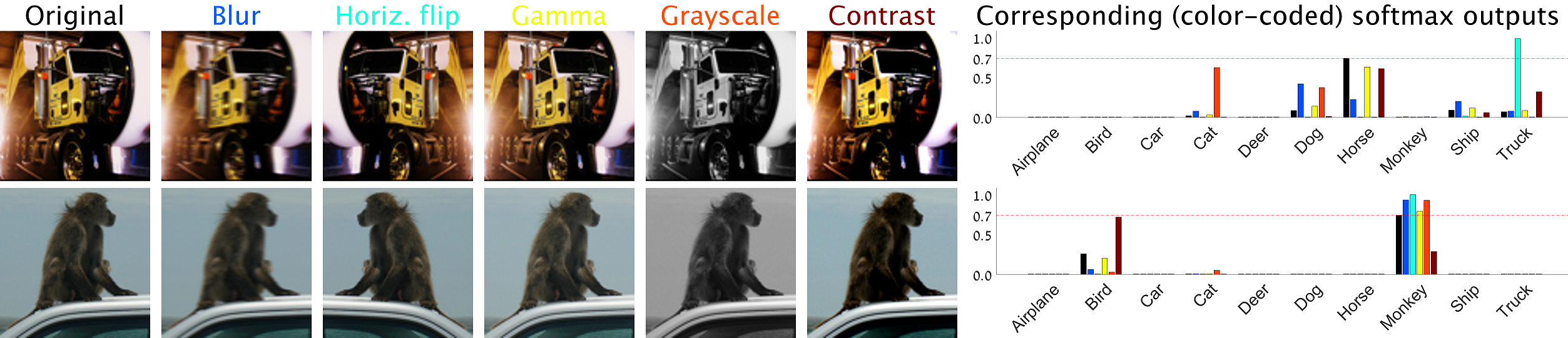
Figure 1: Correctly and incorrectly classified STL-10 images. From left to right: The original images, their transformed versions and their corresponding (color-coded) softmax outputs (obtained using the pre-trained classifier of [1]). While both (original) images obtain the same prediction confidence based on the maximal softmax response (red dashed line), the softmax values of the misclassified (upper) image fluctuate across transformed versions, while those of the correctly classified (lower) image are relatively stable.

1 Introduction

Despite rapid and continuing dramatic improvements in the accuracy of predictors applied to computer vision, these predictors (image classifiers, object detectors, etc.) continue to have a non-trivial error rate. For instance, typical error rate (top-5) of modern classifiers on ImageNet [2] is on the order of 5% [3, 4]. Error rates increase further when an adversarial process generates input images designed to “fool” the classifiers [5, 6]. This observation has led to widespread concerns regarding robustness of neural network classifiers, and sparked interest in building various defenses. In this paper, we pursue a more general goal: error detection. More specifically, enabling endowing a classifier with a reject option – the possibility of signaling lack of confidence in its ability to correctly classify it.

Our work follows two key ideas. The first is to leverage the rich signal in the output of a trained classifier to reason about the likelihood of its prediction being wrong. This approach, intuitively related to the “dark knowledge” ideas [7], goes beyond prior work which narrowly focused on the score/probability of the predicted class. The second idea is to leverage signal from the stability of classifier output under a set of natural image transformations. Intuitively, one can expect that the corresponding changes in output when the prediction is correct may differ in a systematic way from such changes when the prediction is incorrect. For instance, we may expect more invariance to transformations of a correctly classified input, as demonstrated in Fig. 1.

We convert these two intuitions into a specific model for error detection: a predictor mapping the collected outputs under a set of transformations to probability of the original input being misclassified. This approach achieves results significantly exceeding prior state of the art for error detection on a number of data sets.

We can also apply this intuition, and our approach, to the closely related problem of novelty detection. In standard classification settings, all inputs are assumed to correspond to an available output class. However, a visual recognition system deployed in the wild is likely to encounter inputs that belong to novel classes, not included in the training set. In this situation an error is unavoidable, unless the classifier is endowed with a “reject option”.

An additional scenario where the classifier may be expected to reject an input is when that input comes from a domain substantially different from that of the training data (e.g. feeding an image of a digit to a classifier trained to recognize animals). We show that our approach is applicable, and achieves state of the art results, in these novelty detection scenarios as well. To the best of our knowledge, we are the first to establish state of the art in error detection on the ImageNet data set, which is more realistic and larger than the smaller data sets typically used in error detection literature.

2 Related work

The idea of developing reject option for classifiers has been discussed in machine learning literature extensively [8, 9, 10]. We borrow some evaluation methodology from this prior work, in particular [10], but our approach is different from anything proposed there, in particular in our use of image transformations.

The body of recent related work can be broadly divided into error detection methods and novely detection methods. A common and well performing baseline method for both tasks is the Maximal softmax Response (MSR) [11], that interprets the maximal output (the one corresponding to the predicted class) of a softmax classifier as a confidence score. Thresholding this score is then used to detect misclassifications or novel class instances. The intuition is that the output of the original classifier may be poorly calibrated (i.e., will poorly reflect the actual posterior probability $p(\widehat{c}(x)=c|x)$), due to the vagaries of optimizing a particular surrogate loss such as cross entropy, and this thresholding step adjusts the calibration. In [1], calibration is based on estimating density in feature space corresponding to the last layer of a deep neural network before softmax. In order to work well, the approach in [1] requires training the classifier network with a specially modified loss.

In contrast to MSR, we look beyond the maximum of the posterior distribution, and consider a much richer family of detectors (a multilayer perceptron, rather than the simple thresholding in MSR). In contrast to both MSR and [1], we go beyond reasoning about scores on the input at hand, and consider the behavior of the classifier on a set of transformed (perturbed) versions of the input.

A number of methods have been proposed that incorporate reasoning about stability under perturbations into efforts to improve visual classification. In [12] the perturbations consist of applying stochastic dropout to classifier activations. The work in [13] proposes to defend against adversarial attacks [5, 14] using image transformations. However, unlike our work, they employ non-natural transformations, and use those as a pre-processing step rather than a test-time device. This requires retraining the classifier to correct for resulting artifacts. Neither of these efforts is aimed at error detection, which is our goal.

One key distinction between methods for error detection is their required level of access to parameters of the underlying classifier. “White box” methods [1, 15] require full access, and in fact need to re-train the classifier to fit their error detection framework. Other methods are perhaps better characterized as “gray box” requiring some degree of access but not full retraining; this includes the dropout method of [12]. In contrast, MSR, and our proposed approach, do not require any access to the classifier beyond treating it as a “black box” which takes in an image and produces softmax scores for the classes. Thus we can apply our method to endow a fixed, pre-trained classifier with a robust reject option, as we demonstrate in Sec. 4.

3 Confidence from invariance

The techniques we develop below for error and novelty detection are applicable to any classifier trained to output softmax scores for the classes given an image. These techniques require only a “black box” level access to the classifier: the ability to feed it an image and observe the output scores.

3.1 Error detection from class posteriors

A $k$-way classifier $h$ outputs for an input $x$ a $k$-dimensional vector of class scores (logits) $\mathbf{s}^{h}(x)\in\mathbb{R}^{k}$. Using the softmax transformation, the scores can be converted to estimated posterior distribution over classes $\mathbf{p}^{h}(x)=h(x)$, where $p_{c}(x)$ is the estimated conditional probability of $c\in[k]$ being the class of $x$. The prediction is made by selecting $\widehat{c}(x)=\operatorname*{argmax}_{c}p_{c}^{h}(x)$. One could use the value $p_{\widehat{c}}^{h}(x)$ as a measure of confidence in $h$’s decision on $x$. That’s the approach in MSR [11]. However, it has been shown that the entire posterior distribution contains information valuable to the decision making process. This has been called “dark knowledge” in [7].

We propose to directly exploit this information by training a binary classifier, mapping either the scores $\mathbf{s}$ or the posterior $\mathbf{p}$ to the probability of the input (on which this posterior was calculated) being misclassified. To this end, we collect a set of class-labeled examples $(x_{i},y_{i})$, with the corresponding scores $\mathbf{s}^{h}(x_{i})$. Using the trained classifier $h$, we now label each score with the binary error label $e_{i}$, where $e_{i}=0$ if $y_{i}=\widehat{c}(x)$ (correct prediction) and $e_{i}=1$ otherwise (error). Having constructed such a training set, we can learn a binary classifier $d$, producing $d(x)=p\left(e_{i}=1|\mathbf{s}^{h}(x_{i})\right)$, for instance by minimizing the cross entropy loss on the $e_{i}$ labels. To avoid confusion, we will refer to the original (multi-class) classifier $h$ as “classifier”, and to the (binary) classifier $d$ predicting whether $h$ makes an error, as “detector”.

One can expect that $h$ will be more “confident”, and make fewer mistakes on the training data than on future test data; this is the standard overfitting problem. Therefore, we will train $d$ on examples not included in training set for $h$.

3.1.1 Score representation

The score vectors $\mathbf{s}^{h}(x)$ will vary drastically depending on the estimated class distribution. Our detector needs to learn a mapping from these vectors to the probability of error $d(x)$. To facilitate the learning of this mapping, we make the detector invariant to this variation; We convert $\mathbf{s}^{h}$ to a canonical representation by sorting its values. Let $c_{1}$ be the class with the highest $s_{c}(x)$, $c_{2}$ the second highest, etc. In the sorted score representation

$$\tilde{\mathbf{s}}^{h}(x_{i})\,=\,\left[s_{c_{1}}^{h}(x),\ldots,s_{c_{k}}^{h}(x)\right]$$ (1)

the class identity information is lost, but the shape of the distribution is retained.

We can now use $\tilde{\mathbf{s}}$ as input to detector $d$, trained to predict $e_{i}$. In all our experiments the detector is a multi-layer perceptron (MLP).

When the number of classes $k$ is large, learning a detector on top of the full score vector may require too many parameters to learn (or equivalently too many error/non-error examples). To address this we can truncate the representation to $[\tilde{s}_{c_{1}}^{h}(x),\ldots,\tilde{s}_{c_{k^{\prime}}}^{h}(x)]$ for $k^{\prime}<k$. The entire process sketch appears inside the green dashed line in Fig. 3.

3.2 Invariance under transformations

The second component of our approach comes from the expectation that a correct classification decision may/should be invariant to some image transformations applied to the input, while an incorrect one may be less stable. More specifically, we argue that the confidence (here understood as probability of being correct) of prediction $h(x)$ is related to its invariance to a set of “natural” image transformations of $x$. This set includes transformations that can be expected to occur naturally in realistic imaging conditions, while not affecting the semantic content of the image. For instance, horizontal flip since the world is largely laterally symmetric; contrast variation due to environment/sensor variability; etc.

Given a family of image transformations $\cal T$, We can assess the degree of invariance for a given classifier and image pair $(h,x)$, by observing the difference between $\mathbf{p}^{h}(x)$ and $\mathbf{p}^{h}(t(x))$ for $t\in\cal T$, the classifier’s output when fed the original image $x$ vs. $x$ transformed by $t$.

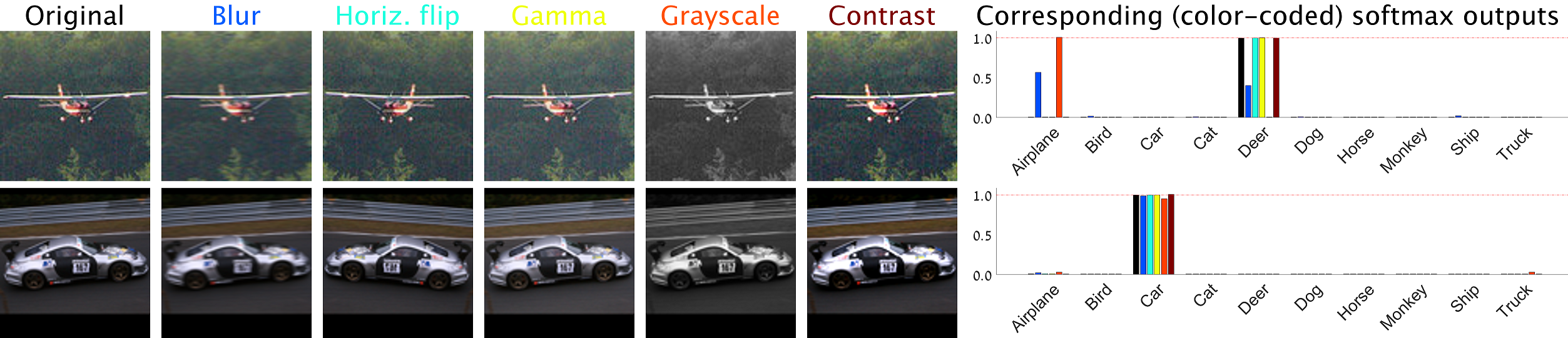
Figure 2: Additional examples of correctly and incorrectly classified STL-10 images. See caption of Fig. 1 for explanation. Note that unlike in Fig. 1, here both images get a very high MSR confidence score (close to 1). Nevertheless, while softmax values of the misclassified (upper) image are inconsistent across transformed versions, those of the correctly classified (lower) image are in concurrence.

As an illustration, Fig. 1 and 2 present two images each, along with their transformed versions under a set of transformations: horizontal blur, horizontal flip, gamma correction, conversion to grayscale, and change in contrast. The right hand side shows the corresponding softmax outputs for each image version (including the original). Note that for the correctly classified images (bottom images, in both figures) the output is fairly consistent across image versions, while for the misclassified one (top images) the transformations induce significant changes in the classifier output. We will now consider computational recipes for converting this intuition into an error detector.

3.2.1 Divergence based error detection

If we expect the correct prediction to come with more stability under transformation $t$, we can quantify stability by computing a measure of difference (divergence) $D\left(\mathbf{p}^{h}(x)||\mathbf{p}^{h}(t(x))\right)$ between the two probability distributions. A widely used choice for $D$ is the Kullback-Leibler divergence $D_{KL}$ [16]. Other choices include the Jensen-Shannon divergence (a symmetrized version of $D_{KL}$), squared distance, or Kolmogorov-Smirnov divergence.

With either of these choices, $D\left(\mathbf{p}^{h}(x)||\mathbf{p}^{h}(t(x))\right)=0$ when the classifier’s output for image $x$ is completely invariant to the image transformation $t$, and it increases as $\mathbf{p}^{h}(t(x))$ diverges more from $\mathbf{p}^{h}(x)$, that is, as the classifier’s prediction on $x$ becomes less invariant under ${t}$.

A straight-forward approach would be to base a detector on thresholding the divergence under transformation $t$ with threshold $\tau$,

$$d^{t}(x)=1\quad\text{if}\quad D\left(\mathbf{p}^{h}(x)||\mathbf{p}^{h}(t(x))\right)\,\geq\,\tau.$$ (2)

The approach as developed thus far considers one transformation at a time. We conjecture (and empirically confirm this conjecture in Sec. 4) that additional power could be derived from jointly considering multiple transformations. Rather than pursue heuristic combination rules for a divergence-based detector, we directly extend the parametric detector framework in Sec. 3.1 to invariance-based scenario with multiple transformations.

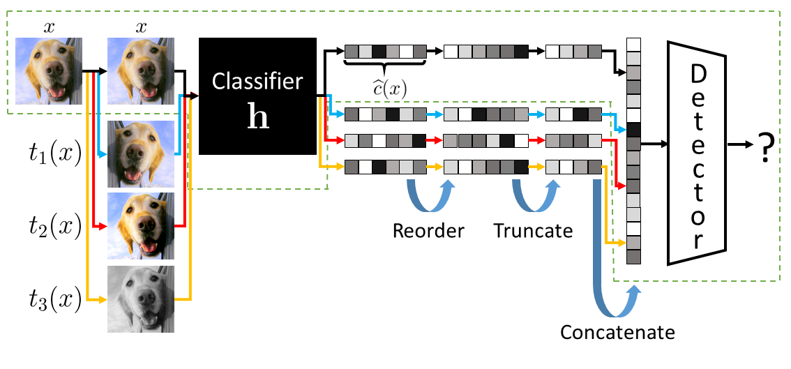
Figure 3: Method overview. Given an image $x$ and a pre-trained classifier $h$, we feed $x$ and several (three, in this example) natural transformations of it into $h$. We jointly re-order all resulting score vectors so that the score vector for $x$ (the original image) is in descending order. We then truncate the score vectors to retain only the $k^{\prime}$ first scores and concatenate them to yield the input to our detector. The green dashed line delineates our approach when used without the transformations (denoted by MLP in Sec. 4).

3.3 Combining confidence and invariance

Given a set of transformations $\mathcal{T}=\{t_{1},\ldots,t_{m}\}$ and the fixed classifier $h$, we can compute, for an image $x$, the set of output scores $\mathbf{s}^{h}(t_{0}(x)),\mathbf{s}^{h}(t_{1}(x)),\ldots,\mathbf{s}^{h}(t_{m}(x))$, where the “null transformation” $t_{0}$ is identity (i.e., the original input).

We then jointly order all score vectors $\mathbf{s}^{h}(t_{j}(x)),~{}t_{j}\in\cal T$ by sorting the scores of the original input; finally, all the sorted scores are truncated by keeping only the first $k^{\prime}\leq k$ values. Conceptually, this forms a re-ordered, truncated $m+1\times k^{\prime}$ matrix of scores. Please see Fig. 3, depicting this process for $m=3$, $k=6$ and $k^{\prime}=4$.

3.4 Novelty detection

When the true label of an image fed to a classifier lies outside the classifier’s $k$ possible classes, the predicted class is guaranteed to be incorrect. A mechanism to detect such incidents is called novelty detector. In this work, we refine the notion of novelty into two scenarios, and use our method to detect each of them. A crucial distinction from the error detection task above is that here, we can not possess labeled training examples covering the class distribution of novel images.

3.4.1 Novel Domains

The first novelty scenario (previously explored in, e.g., [1, 11]) is the domain novelty (also known as out-of-distribution (OOD) novelty), where a classifier trained on a certain domain (e.g. STL-10 dataset of objects) is fed with images from a different domain (e.g. the SVHN [17] dataset of street numbers, see top row of Fig. 4).

Figure 4: Novel (misclassified) image from SVHN and correctly classified STL-10 image. See caption of Fig. 1 for explanation.

To detect OOD images, we use the same framework explained in Sec. 3.3. We assume that we have access to a data set of images from a domain different from what the classifier was trained on, which can generally be different from the domains that may be encountered in the future. For instance, given a hand-written digit classifier, we can train the error detector by using images of objects to simulate novel inputs. We can then use this detector to detect images from other novel domains (e.g. animals).

3.4.2 Novel Classes

The second novelty scenario we discuss here is more realistic. After a classifier is trained to distinguish between $k$ classes and is deployed, it will eventually encounter input images that come from classes beyond those $k$ (but still from the same domain). In this scenario, novelty detector must identify images from the unfamiliar classes, both to prevent errors and, in some applications, to provide a mechanism for active learning (soliciting labels for examples of unfamiliar classes). Our method can be employed for this case too.

To overcome the training examples problem in this case, we take a slightly different approach, and use a hold-out partition of the original training set for the classifier $h$. Specifically, we hold out a subset of classes, say $\tilde{k}<k$, and train a classifier $\tilde{h}$ (with the same architecture) on the remaining classes $c\leq\tilde{k}$. We then train an error/novelty detector as in the OOD scenario, but using examples from the heldout classes as OOD examples. Once the detector $d$ is trained, we can apply it to detect novelty for the original, full-set classifier $h$. We elaborate on this procedure in Sec. 4.4.3.

4 Experiments

In our experiments we use three primary data sets: STL-10 [18], CIFAR-100 [19], and ImageNet [2], as base data sets on which the visual classifier (whose errors we will want to detect) is trained. Each of these is roughly an order of magnitude larger than the previous one in terms of both number of examples and the number of classes. This is to confirm that the proposed method generalized across such parameters of the data set/classification task.

We demonstrate results with different classifiers, including a competitive Inception-ResNet classifier. Our experiments include both the basic error detection task and multiple novelty detection scenarios. We compare, to the extent possible, to previously proposed methods, across a range of meaningful metrics; in contrast to image classification, there is no clear single way to evaluate error detection or novelty detection.

4.1 Evaluation Measures

We use the following measures to evaluate and compare performance.

Area Under Receiver Operating Characteristic Curve (AUROC) relies on the ROC curve (true-positive vs. false positive rates for all possible thresholds on a detector’s output). The area under the ROC curve is invariant to the “polarity” of our detection task - whether we detect correct or incorrect classifications - because the curves for these two definitions are symmetric. However, the AUROC is dependent on the ratio of incorrect vs. correct classifications, hence this ratio in the test set should be maintained constant when comparing different detectors.

Coverage vs. Accuracy Curve (CAC) that relates to using the reject option for classification. Each point $(coverage,accuracy)$ in the curve reflects the anticipated $accuracy$ when using detector $d$ to keep only the $coverage$ portion of classifications corresponding to the lowest error detection score $d(x)$. Similar to AUROC, we also use the area under the CAC (AUCAC) to evaluate performance.

4.2 Error detection: Experimental setup

Throughout our experiments we use a fully connected MLP detector that has two hidden layers of width 70, each followed by RELU nonlinearity, and a batch normalization layer. We train our detector using asymmetric cross-entropy loss, reweighting examples to correct for the binary class (correct / incorrect) imbalance, and with dropout probability $0.5$ in both hidden layers.

We used the following set of natural image transformations $\mathcal{T}$ throughout our experiments:

Horizontal flip: Flipping the image on the horizontal axis. Horizontal blur: Blurring the image with a horizontal blur kernel. We used a magnitude of 3 pixels in our implementation. Converting to gray-scale: Overriding all three channels ($R,G,B$) of each image pixel with $0.299\times R+0.587\times G+0.114\times B$. Contrast enhancement: Increasing image contrast by $1.3$. Gamma correction: Raising each image pixel to the power of $0.85$.

To avoid the problem of fitting our detector to training-set images outputs, we train it using validation-set images. To this end, we split the originally given validation set to two subsets, and use them as training and validation sets for our detector. As explained in Sec. 3.3, when using an MLP, we reorder and clip to length $k^{\prime}$ the output vectors $\mathbf{s}^{h}(t_{j}(x))$ corresponding to each image $t_{j}(x)$, before concatenating them into a single input vector for our detector. We use $k^{\prime}=5,10,20$ when applying our method to the STL-10, CIFAR-100 and ImageNet data-set, respectively.

In training error and novelty detectors, we use data augmentation, by randomly applying horizontal flip and random brightness and contrast adjustments (and for ImageNet, also a random crop). When constructing the MLP+Invariance representations, the (fixed) transformations in $\mathcal{T}$ are applied to an input image after it has been obtained using the data augmentation pipeline.

	Original	Flip	Gamma	Contrast	Blur	Gray scale	ALL
MSR [11]	0.807	-	-	-	-	-	-
Ours, KL divergence	-	0.809	0.787	0.798	0.797	0.708	-
Ours, MLP	0.813	0.834	0.821	0.824	0.825	0.822	0.846

Table 1: Error detection using different image transformations, STL-10. AUROC values of detectors based on scores of different image transformations. Middle row values correspond to directly using the KL-divergence score, while bottom row values are obtained using MLP on top of the logits. All detectors are applied on the Regular classifier of [1].

4.3 Error detection: results

STL-10 We evaluated the performance gains of the different components of our method using a pre-trained STL-10 image classifier (trained by [1]) with $70\%$ accuracy, and present the result in table 1. We followed Eq. 2 and directly used the KL-divergences between classifier outputs corresponding to the original images vs. one of the transformations in $\mathcal{T}$, as an error detection mechanism. This by itself (middle row) gave comparable performance to MSR. Using other divergence measures mentioned in Sec. 3.2 gave results which were consistent with those of KL-divergence. We omit those divergences from further discussion.

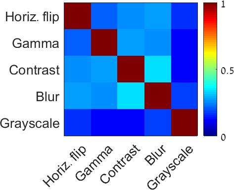
Figure 5: Correlation between KL-divergences for different $t\in\mathcal{T}$.

Next, we evaluate the power of combining several image transformations. As a diagnostic experiment, we compute correlation coefficients between KL-divergence values (between posteriors for the original input and the posterior for the result of transformation $t$) computed for different $t\in\mathcal{T}$. As shown in Fig. 5), many of these correlations are low, indicating that the information provided by outputs on different $t$s is not completely redundant.

The bottom row of table 1 presents the performance achieved when using an MLP and feeding it with the classifier’s output corresponding to (1) the original image alone (left column), (2) the original image and one transformed image (middle columns) and (3) all image versions (right column). This exploits the full power of our method and achieves a significant increase in error detection performance (approximately 4 points gain in AUROC compared to MSR or KL-divergence).

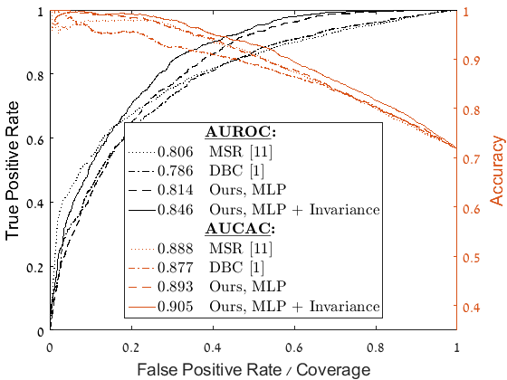
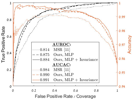
Figure 6: Error detection on the STL-10 (left) and ImageNet top-5 (right) classification tasks. ROC and CAC corresponding to error detection using MSR [11] and our method, with and without using invariance to image transformations. For STL-10, we also plot the curves for DBC [1], and leave out the plot for MC-dropout [12], which performs similarly to MSR (see table 2). Values in the legend correspond to Area Under Curves.

More extensive comparison of our method to MSR [11], MC-dropout [12] and the SOTA method by Mandelbaum and Weinshall [1] on STL-10 are shown in Tables 2 and 3. Our evaluation included pre-trained classifiers used in [1], that differ in the loss function they utilized; The Regular classifier used only the cross entropy loss. Dist. and AT both employ the cross-entropy loss, but augment it with a features embedding term or the adversarial loss term of [14], respectively. The latter two loss functions require retraining the classifier to improve the performance of DBC, and thus are by design favorable to DBC (and in that sense do not satisfy our desired black box treatment of the classifier).

The resulting ROC and CAC (corresponding to the ‘Regular’ classifier) appear in Fig. 6 (left). AUROC and AUCAC values for all three classifiers are presented in tables 2 and 3, respectively.

	STL-10			CIFAR-100
	Regular	Dist.	AT	Regular	Dist.	AT
Accuracy (%)	71.8	71.9	70	58.8	57.8	59.1
MSR [11]	0.806	0.772	0.813	0.834	0.83	0.842
MC-dropout[12]	0.803	0.78	0.809	0.834	0.83	0.847
DBC [1]	0.786	0.816	0.866	0.782	0.852	0.858
Ours, MLP	0.814	0.789	0.817	0.848	0.833	0.846
Ours, MLP+Inv.	0.846	0.836	0.868	0.864	0.857	0.869

Table 2: Error detection AUROC on pre-trained classifiers of [1]. Comparing our method (bottom row) to MSR [11], MC-Dropout [12] and the method of Mendelbaum and Weinshall [1], when tested on classifiers trained by [1].

	STL-10			CIFAR-100
	Regular	Dist.	AT	Regular	Dist.	AT
Accuracy (%)	71.8	71.9	70	58.8	57.8	59.1
MSR [11]	0.888	0.862	0.883	0.825	0.815	0.832
MC-dropout[12]	0.89	0.869	0.883	0.827	0.815	0.834
DBC [1]	0.877	0.892	0.904	0.772	0.824	0.833
Ours, MLP	0.893	0.874	0.887	0.832	0.817	0.834
Ours, MLP+Inv.	0.905	0.9	0.903	0.839	0.827	0.843

Table 3: Error detection AUCAC on pre-trained classifiers of [1]. Different measure for the same experiment as in table 2.

Our method achieves the best performance on all three classifiers (except for one metric in one experiment). Note that while our detector can be used on any given, pre-trained, classifier, it achieves SOTA performance even on classifiers that were especially modified by [1] (the AT and Dist. configurations).

CIFAR-100 Next, we performed an evaluation on the CIFAR-100 dataset. We followed the same experiment as before, and used the three pre-trained classifier of the DBC method [1]. A comparison of AUROC and AUCAC values is presented in tables 2 and 3, respectively. Here too, our method achieves SOTA performance on all classifiers, including those modified by DBC.

ImageNet Finally, we evaluated our method’s performance when applied to the ILSVRC-2012 ImageNet classification task. We used a pre-trained Inception-ResNet-v2 model [3] that achieves $81\%$ and $95.5\%$ top-1 and top-5 accuracies, respectively. As before, we used part of ImageNet’s validation set to train our detector, and evaluated its performance on the remaining part ($20\%$ in this experiment). Fig. 6 (right) presents ROC and CAC for detecting errors in the top-5 classification task. We compare curves corresponding to our method (with and without employing transformations) and MSR. Table 4 presents the corresponding AUROC and AUCAC values. Due to the scale of ImageNet, we did not compare to “white box” methods that require either extensive re-training (DBC) or extensive computation (MC-dropout).

	Top-1	Top-5
Accuracy (%)	81	95.5
MSR [11]	0.842/0.936	0.806 /0.983
Ours, MLP	0.866/0.948	0.877/0.991
Ours, MLP+Inv.	0.875/0.952	0.884/0.991

Table 4: Error detection performance on a pre-trained Inception-ResNet-v2 ImageNet classifier of [3]. AUROC/AUCAC values of MSR compared to our method, with (bottom row) and without (middle row) employing invariance to image transformations.

4.4 Novelty detection

We evaluated the performance of our method when used for detecting novelty of both types described in Sec. 3.4, namely novel domain (OOD) and novel classes. Prior to performing the evaluation, we had to decide how to treat cases of non-novel images that are misclassified by the classifier (i.e. errors, in the context of error-detection). We took an operational point of view and chose to treat these cases as novel (hence a novelty detector should detect them), rather than ignore them.

4.4.1 Domain novelty: setup

We fed the three pre-trained STL-10 classifiers of DBC (Regular, Dist. and AT) with images from either the CIFAR-100 or the SVHN data-sets. In both cases, half the images came from the original data-set (STL-10) and the other half from the novel data-set (CIFAR-100 or SVHN).

1. Define ${\cal C}_{N}\subset{\cal C}$ of size $S_{N}=|{\cal C}_{N}|$, simulating novel, unknown classes. Denote by ${\cal C}_{F}$ its complementary subset of familiar, known classes ${\cal C}_{F}={\cal C}\setminus{\cal C}_{N}$.

2. Train a classifier $h$ using only images from classes $\in{\cal C}_{F}$

3. Set $T_{F}=\{\}$, a training set containing output scores corresponding to images and their transformations.

4. for All possible subsets $\tilde{{\cal C}}_{N}\subset{\cal C}_{F}$ of size $S_{N}$ (and their complementaires, $\tilde{{\cal C}}_{F}$) do

      

(a)

Train a classifier $\tilde{h}$ using only images from classes $\in\tilde{{\cal C}}_{F}$

(b)

Feed $\tilde{h}$ with images from all familair classes (${\cal C}_{F}$) and their transformed versions (Note that $S_{N}$ of the classes in ${\cal C}_{F}$ are unkonwn to $\tilde{h}$). Add the corresponding output logits of $\tilde{h}$ to the training set $T_{F}$.

end for

Train an MLP novelty detector using $T_{F}$. 6. Evaluate the detector performance on classifier $h$, by feeding it with images from all classes $\in{\cal C}$ (and their transformed versions).

Algorithm 1 The training procedure used for class novelty experiments on STL-10. $\mathcal{C}$ is the complete set of classes in the data set.

	SVHN is novel			CIFAR-100 is novel
	Regular	Dist.	AT	Regular	Dist.	AT
Accuracy (%)	35.9/50	35.9/50	35.0/50	35.9/50	35.9/50	35.0/50
MSR [11]	0.818	0.798	0.745	0.802	0.775	0.846
DBC [1]	0.813	0.854	0.893	0.783	0.849	0.883
MC-dropout [12]	0.819	0.808	0.743	0.804	0.792	0.846
Ours	0.825	0.847	0.902	0.818	0.837	0.879
Ours, Cross-train	0.898	0.889	0.914	0.86	0.874	0.907

Table 5: Novelty detection, across domains. The STL-10 pre-trained classifiers of [1] were fed with images from SVHN and CIFAR100 datasets. Values represent AUROC on validation sets constituting 50% novel images (hence the maximum accuracy is 50%). Misclassified STL-10 images were considered novel for this experiment. Ours, Cross-train is our detector when trained on novel images from the non-participating domain - CIFAR-100 for the ‘SVHN is novel’ experiment, and vice versa.

4.4.2 Domain novelty: results

Table 5 presents AUROC results for detecting novel images. Note that in this case, training our detector on familiar domain images only (denoted by ‘Ours’) yields inferior results. This problem is solved, however, by augmenting our detector training set with images from a domain with which the classifier at hand is unfamiliar (‘Ours, Cross-train’).

Novel classes (${\cal C}_{N}$)	Classifier’s	MSR [11]	Ours, MLP	Ours, MLP+Inv.
	accuracy (%)
(0)-Airplane, (1)-Bird	57.4	0.732/0.646	0.734/0.648	0.774/0.68
(2)-Car, (3)-Cat	54.5	0.717/0.622	0.724/0.62	0.78/0.659
(4)-Deer, (5)-Dog	57.9	0.718/0.65	0.722/0.652	0.772/0.685
(6)-Horse, (7)-Monkey	54.5	0.724/0.627	0.722/0.63	0.769/0.662
(8)-Ship, (9)-Truck	56.3	0.655/0.553	0.637/0.548	0.691/0.577
(0)-Airplane, (5)-Dog	59.1	0.724/0.655/	0.73/0.663	0.768/0.683
(3)-Cat, (6)-Horse	55	0.725/0.636	0.723/0.635	0.776/0.668
(4)-Deer, (8)-Ship	57	0.706/0.63	0.709/0.639	0.762/0.666
(2)-Car, (7)-Monkey	60.8	0.708/0.648	0.712/0.654	0.749/0.67
(1)-Bird, (9)-Truck	61.6	0.737/0.677	0.746/0.685	0.782/0.705
Average	57.4	0.715/0.634	0.716/0.637	0.762/0.666
STD	2.5	0.023/0.033	0.03/0.035	0.027/0.034

Table 6: Novelty detection, within domain (novel classes). Each row corresponds to different classes chosen to simulate novelty. From left to right: Chosen classes, classifier’s accuracy on the 8 non-novel classes and AUROC/AUCAC values for MSR and our method, without and with employing classifier’s invariance to image transformations. Average and STD values appear in the bottom two rows.

4.4.3 Class novelty: setup

To simulate this scenario and evaluate our detector’s performance in this case, we use the STL-10 data-set with its 10 classes ($|{\cal C}|=10$) and follow the procedure in Alg. 6.

In this experiment we used a simple architecture (available on-line in [20]) as our classifiers $h$ and $\tilde{h}$. To this end, we downscaled the 96x96 pixels STL-10 images to 32x32 pixels before feeding them into our classifiers. This architecture has 2 convolutional blocks, each constituting a max-pool and a batch-normalization layer, followed by two fully connected layers. We trained each of the classifiers $h$ (for a given choice of ${\cal C}_{N}$) and $\tilde{h}$ (for all classes subsets $\tilde{{\cal C}}_{F}$ induced by this chosen ${\cal C}_{N}$) for two hours (in parallel), reaching the accuracy of approximately $55\%-60\%$ on non-novel classes.

4.4.4 Class novelty: results

We repeated the experiment in Sec. 4.4.3 for ten, arbitrarily chosen pairs of classes that simulate novelty. AUROC and AUCAC values are reported in table 6, along with average and standard deviation values.

Using our method without the invariance part achieves comparable results to the other “black-box” method, MSR. However, exploiting the full power of our method brings a major leap in performance in this realistic novelty scenario.

5 Conclusion

We have presented a new approach to error and novelty detection in visual classification, based on analysis of stability of classifier’s output under a set of natural input transformations. We use a multi-layer perceptron detector whose input is the output scores of a visual classifier. In contrast to many previous efforts, our approach only requires a black box level access to the classifier, and thus can be applied to any off the shelf, pre-trained classifier. We demonstrate new state of the art achieved by our method on both error detection and novelty (novel domain or novel class) detection on a number of data sets, including ImageNet paired with a modern ResNet-based classifier. We believe the notion of classifier’s invariance to natural image transformations can be further exploited in the future, for example by incorporating it into the training procedure of visual classifiers, in an attempt to yield accuracy gains.

References

- [1] Mandelbaum, A., Weinshall, D.: Distance-based Confidence Score for Neural Network Classifiers. ArXiv e-prints (September 2017)
- [2] Russakovsky, O., Deng, J., Su, H., Krause, J., Satheesh, S., Ma, S., Huang, Z., Karpathy, A., Khosla, A., Bernstein, M., Berg, A.C., Fei-Fei, L.: ImageNet Large Scale Visual Recognition Challenge. International Journal of Computer Vision (IJCV) 115(3) (2015) 211–252
- [3] Szegedy, C., Ioffe, S., Vanhoucke, V.: Inception-v4, inception-resnet and the impact of residual connections on learning. In: ICLR workshop. (2016)
- [4] Huang, G., Liu, Z., Weinberger, K.Q., van der Maaten, L.: Densely connected convolutional networks. In: CVPR. (2017)
- [5] Szegedy, C., Zaremba, W., Sutskever, I., Bruna, J., Erhan, D., Goodfellow, I., Fergus, R.: Intriguing properties of neural networks. arXiv preprint arXiv:1312.6199 (2013)
- [6] Nguyen, A., Yosinski, J., Clune, J.: Deep neural networks are easily fooled: High confidence predictions for unrecognizable images. In: CVPR. (2015)
- [7] Hinton, G., Vinyals, O., Dean, J.: Distilling the knowledge in a neural network. arXiv preprint arXiv:1503.02531 (2015)
- [8] Bartlett, P.L., Wegkamp, M.H.: Classification with a reject option using a hinge loss. Journal of Machine Learning Research 9(Aug) (2008)
- [9] Cortes, C., DeSalvo, G., Mohri, M.: Boosting with abstention. In: Advances in Neural Information Processing Systems. (2016)
- [10] Geifman, Y., El-Yaniv, R.: Selective classification for deep neural networks. In: Advances in neural information processing systems. (2017)
- [11] Hendrycks, D., Gimpel, K.: A Baseline for Detecting Misclassified and Out-of-Distribution Examples in Neural Networks. ArXiv e-prints (October 2016)
- [12] Gal, Y., Ghahramani, Z.: Dropout as a Bayesian approximation: Representing model uncertainty in deep learning. arXiv:1506.02142 (2015)
- [13] Guo, C., Rana, M., Cissé, M., van der Maaten, L.: Countering adversarial images using input transformations. In: ICLR. (2018)
- [14] Goodfellow, I.J., Shlens, J., Szegedy, C.: Explaining and Harnessing Adversarial Examples. ArXiv e-prints (December 2014)
- [15] Wang, W., Wang, A., Tamar, A., Chen, X., Abbeel, P.: Safer classification by synthesis. arXiv preprint arXiv:1711.08534 (2017)
- [16] Cover, T.M., Thomas, J.A.: Elements of information theory. John Wiley & Sons (2012)
- [17] Netzer, Y., Wang, T., Coates, A., Bissacco, A., Wu, B., Ng, A.Y.: Reading digits in natural images with unsupervised feature learning. In: NIPS workshop on deep learning and unsupervised feature learning. Volume 2011. (2011) 5
- [18] Coates, A., Ng, A., Lee, H.: An analysis of single-layer networks in unsupervised feature learning. In: AISTATS. (2011)
- [19] Krizhevsky, A., Nair, V., Hinton, G.: Cifar-100 (canadian institute for advanced research). In: AISTATS. (2011)
- [20] TensorFlow: Convolutional Neural Networks TensorFlow. https://github.com/tensorflow/models/tree/master/tutorials/image/cifar10/ Accessed: 2018-03-04.