Recursive Optimization of Convex Risk Measures:
Mean-Semideviation Models

Abstract

We develop recursive, data-driven, stochastic subgradient methods for optimizing a new, versatile, and application-driven class of convex risk measures, termed here as mean-semidevi- ations, strictly generalizing the well-known and popular mean-upper-semideviation. We introduce the $\textit{MESSAGE}^{p}$ algorithm, which is an efficient compositional subgradient procedure for iteratively solving convex mean-semideviation risk-averse problems to optimality, and constitutes a parallel variation of the recently developed, general purpose $T$-SCGD algorithm of Yang, Wang & Fang (Yang et al., 2018). We analyze the asymptotic behavior of the $\textit{MESSAGE}^{p}$ algorithm under a flexible and structure-exploiting set of problem assumptions, which reveal a well-defined trade-off between the expansiveness of the random cost and the smoothness of the mean-semideviation risk measure under consideration. In particular:

• Under appropriate stepsize rules, we establish pathwise convergence of the $\textit{MESSAGE}^{p}$ algorithm in a strong technical sense, confirming its asymptotic consistency.

• Assuming a strongly convex cost, we show that, for fixed semideviation order $p>1$ and for $\epsilon\in\left[0,1\right)$, the $\textit{MESSAGE}^{p}$ algorithm achieves a squared-${\cal L}_{2}$ solution suboptimality rate of the order of ${\cal O}(n^{-\left(1-\epsilon\right)/2})$ iterations, where, for $\epsilon>0$, pathwise convergence is simultaneously guaranteed. This result establishes a rate of order arbitrarily close to ${\cal O}(n^{-1/2})$, while ensuring strongly stable pathwise operation. For $p\equiv 1$, the rate order improves to ${\cal O}(n^{-2/3})$, which also suffices for pathwise convergence, and matches previous results.

• Likewise, in the general case of a convex cost, we show that, for any $\epsilon\in\left[0,1\right)$, the $\textit{MESSAGE}^{p}$ algorithm with iterate smoothing achieves an ${\cal L}_{1}$ objective suboptimality rate of the order of ${\cal O}(n^{-\left(1-\epsilon\right)/\left(4\mathds{1}_{\left\{p>1\right\}}+4\right)})$. This result provides maximal rates of ${\cal O}(n^{-1/4})$, if $p\equiv 1$, and ${\cal O}(n^{-1/8})$, if $p>1$, matching the state of the art, as well.

Finally, we discuss the superiority of the proposed framework for convergence, as compared to that employed earlier in (Yang et al., 2018), within the risk-averse context under consideration. By performing careful analysis and by constructing non-trivial counterexamples, we explicitly demonstrate that the class of mean-semideviation problems supported herein is strictly larger than the respective class of problems supported in (Yang et al., 2018). As a result, this work establishes the applicability of compositional stochastic optimization for a significantly and strictly wider spectrum of convex mean-semideviation risk-averse problems, as compared to the state of the art. This fact justifies the purpose of our work from this perspective, as well.

   Keywords. Risk-Averse Optimization, Risk-Aware Learning, Risk Measures, Mean-Upper-Semi- deviation, Stochastic Optimization, Stochastic Gradient Descent, Compositional Optimization.

1 Introduction

During the last almost twenty years, many significant advances have been made in the now relatively mature area of risk-averse modeling and optimization. These primarily include the fundamental axiomatization and theoretical characterization of risk functionals, also commonly known as risk measures (Kijima and Ohnishi, 1993; Rockafellar and Uryasev, 1997; Artzner et al., 1999; Ogryczak and Ruszczyński, 1999, 2002; Rockafellar and Uryasev, 2002; Rockafellar et al., 2003, 2006; Ruszczyński and Shapiro, 2006b; Shapiro et al., 2014), as well as extensive analysis in the context of risk-averse stochastic programs in both static and sequential decision making problem settings (Rockafellar and Uryasev, 1997; Föllmer and Schied, 2002; Rockafellar et al., 2003, 2006; Ruszczyński and Shapiro, 2006a; Collado et al., 2012; Çavuş and Ruszczyński, 2014a; Asamov and Ruszczyński, 2015; Dentcheva and Ruszczyński, 2017; Grechuk and Zabarankin, 2017; Shapiro, 2017; Fan and Ruszczyński, 2018). The importance of building a well structured theory of risk is motivated by its natural and intuitive relevance to problems from a large variety of applied domains. Arguably the oldest, archetypical application of risk is in Finance (Kijima and Ohnishi, 1993; Rockafellar and Uryasev, 1997; Andersson et al., 2001; Krokhmal et al., 2001; Chen and Wang, 2008; Shang et al., 2018), which has decisively driven pioneering research in risk-averse modeling and optimization, from its very birth, probably dating back to the work of Markowitz (Markowitz, 1952), to present. Other applications of risk may be found in both classical and contemporary domains such as Energy (Moazeni et al., 2015; Bruno et al., 2016; Jiang and Powell, 2016), Wireless Networks (Ma et al., 2018), Inventory Optimization (Ahmed et al., 2007; Chen et al., 2007; Xinsheng et al., 2015) and Supply Chain Management (Gan et al., 2004; Sawik, 2016), to name a few.

Most recently, the development of effective computational methods for applying risk-averse optimization to actual problems has also been attracting considerable attention; see, e.g., (Ruszczyński, 2010; Çavuş and Ruszczyński, 2014b; Moazeni et al., 2017; Tamar et al., 2017; Dentcheva et al., 2017; Huang and Haskell, 2018; Jiang and Powell, 2017; Yu et al., 2018). This line of work can be divided between sequential settings (Çavuş and Ruszczyński, 2014b; Moazeni et al., 2017; Tamar et al., 2017; Huang and Haskell, 2018; Jiang and Powell, 2017; Yu et al., 2018), and static settings (Tamar et al., 2017; Dentcheva et al., 2017), for a variety of different problem characteristics. Computational recipes also vary. For instance, (Ruszczyński, 2010) and (Çavuş and Ruszczyński, 2014b) develop and analyze variations of the well known value and policy iteration algorithms of risk-neutral dynamic programming; (Moazeni et al., 2017) proposes a method for risk-averse nonstationary direct parametric policy search for finite horizon problems; (Tamar et al., 2017), (Dentcheva et al., 2017) and (Yu et al., 2018) rely on the so-called Sample Average Approximation (SAA) approach (Shapiro et al., 2014), where an appropriately constructed empirical estimate of the original objective is used as a surrogate to that of the original stochastic program, assuming existence of a sufficiently large sample of the processes introducing uncertainty into the corresponding risk-averse objective; (Huang and Haskell, 2018) and (Jiang and Powell, 2017) consider an Approximate Dynamic Programming (ADP) (Powell, 2011) approach, where sequential finite state/action risk-averse stochastic programs are tackled via stochastic approximation (Kushner and Yin, 2003).

Following this recent trend, this paper proposes and rigorously analyzes recursive stochastic subgradient methods for an important class of static, convex risk-averse stochastic programs. In a nutshell, we make the following contributions:

1. Following the Mean-Risk Model paradigm (Shapiro et al., 2014), we introduce a new class of convex risk measures, called mean-semideviations. These strictly generalize the well known mean-upper-semideviation risk measure, and are constructed by replacing the positive part weighting function of the latter by another nonlinear map, termed here as a risk regularizer, obeying certain properties. Mean-semideviations share the same core analytical structure with the mean-upper-semideviation risk measure; however, they are much more versatile in applications. We study mean-semideviations in terms of their basic properties, and we present a fundamental constructive characterization result, demonstrating their generality. Specifically, we show that the class of all mean-semideviation risk measures is almost in one-to-one correspondence with the class of cumulative distribution functions (cdfs) of all integrable random variables. This result provides an analytical device for constructing mean-semideviations with desirable characteristics, starting from any cdf of the aforementioned type. The flexibility and effectiveness of mean-semideviations are explicitly demonstrated on a classical, chance-constrained newsvendor model, as well.

2. We introduce the $\textit{MESSAGE}^{p}$ (MEan-Semideviation Stochastic compositionAl subGradient dEscent of order $p$) algorithm, an efficient, data-driven Stochastic Subgradient Descent (SSD) -type procedure for iteratively solving convex mean-semideviation risk-averse problems to optimality. The $\textit{MESSAGE}^{p}$ algorithm constitutes a parallel variation of general purpose T-level Stochastic Compositional Gradient Descent ($T$-SCGD) algorithm, recently developed in (Yang et al., 2018), under a generic theoretical framework. Although risk-averse optimization is listed in (Yang et al., 2018) as a potential application of stochastic compositional optimization for the mere case of mean-upper-semideviations, this work is the first to propose a general algorithm, applicable to any mean-semideviation model of choice.

3. We analyze the asymptotic behavior of the $\textit{MESSAGE}^{p}$ algorithm under a new, flexible and structure-exploiting set of problem assumptions, which reveal a well-defined trade-off between the expansiveness of the random cost and the smoothness of the mean-semideviation risk measure under consideration. In particular, under our proposed structural framework:

   • Under appropriate stepsize rules, we establish pathwise convergence of the $\textit{MESSAGE}^{p}$ algorithm in a strong technical sense, confirming its asymptotic consistency.

   • Assuming a strongly convex cost function, the convergence rate of the $\textit{MESSAGE}^{p}$ algorithm is studied in detail. More specifically, we show that, for fixed semideviation order $p>1$ and for $\epsilon\in\left[0,1\right)$, the $\textit{MESSAGE}^{p}$ algorithm achieves a squared-${\cal L}_{2}$ solution suboptimality rate of the order of ${\cal O}(n^{-\left(1-\epsilon\right)/2})$ iterations, where, for $\epsilon>0$, pathwise convergence is simultaneously guaranteed. Thus, this new result establishes a rate of order arbitrarily close to ${\cal O}(n^{-1/2})$, also ensuring strongly stable pathwise operation of the $\textit{MESSAGE}^{p}$ algorithm. In the simpler case where the semideviation order is chosen as $p\equiv 1$, the rate order of the proposed algorithm improves to ${\cal O}(n^{-2/3})$, which is sufficient for pathwise convergence as well, and matches previous results in the related literature (Wang et al., 2017).

   • For the general case of a convex cost, we show that, for any $\epsilon\in\left[0,1\right)$, the $\textit{MESSAGE}^{p}$ algorithm with iterate smoothing achieves an ${\cal L}_{1}$ objective suboptimality rate of the order of ${\cal O}(n^{-\left(1-\epsilon\right)/\left(4\mathds{1}_{\left\{p>1\right\}}+4\right)})$. As in the strongly convex case, for $\epsilon>0$, pathwise convergence is also simultaneously guaranteed. For $\epsilon\equiv 0$, this result provides maximal rates of ${\cal O}(n^{-1/4})$, if $p\equiv 1$, and ${\cal O}(n^{-1/8})$, if $p>1$, matching the state of the art, as well.

4. We discuss the superiority of the proposed framework for convergence, as compared to that employed earlier in (Yang et al., 2018), within the risk-averse context under consideration. By performing careful analysis and by constructing non-trivial counterexamples, we explicitly demonstrate that the class of mean-semideviation problems supported herein is strictly larger than the respective class of problems supported in (Yang et al., 2018). As a result, this paper establishes the applicability of compositional stochastic optimization for a significantly and strictly wider spectrum of convex mean-semideviation risk-averse problems, as compared to the state of the art. This fact justifies the purpose of our work from this perspective, as well.

Our contributions, briefly outlined above, are now discussed in greater detail. We also briefly explain how our work relates to and is placed within the existing literature.

1.1 Mean-Semideviation Risk Measures

Mean-semideviation risk measures, as proposed and developed in this work, constitute a new class of risk measures where, given a random cost, the corresponding dispersion measure (the term penalizing the “mean” part of a mean-risk functional) is defined as the ${\cal L}_{p}$-norm of a nonlinear, one-dimensional map of the centered cost, or, in other words, its central deviation. This map is called a risk regularizer, and possesses certain analytical properties: convexity, nonnegativity, monotonicity and nonexpansiveness. Dispersion measures with this structure are suggestively called generalized semideviations.

This terminology originates from the presence of the positive part function $\left(\cdot\right)_{+}\triangleq\max\left\{\cdot,0\right\}$, which is the simplest, prototypical example of a risk regularizer, in the corresponding dispersion measure of the well known mean-upper-semideviation risk measure (Shapiro et al., 2014), i.e., the upper-(central)-semideviation. Mean-semideviations are much more versatile, however, since different choices for the involved risk regularizer correspond to different rules for ranking the relative effect of both riskier (higher than the mean) and less risky (lower than the mean) events, corresponding to specific regions in the range of the (centered) cost. As a result, the choice of the risk regularizer affects the general quality and the roughness/stability of an optimal random cost, in a decision making setting. Consequently, owing to their versatility, mean-semideviations are practically appealing as well, because they are parametrizable and they may incorporate domain specific knowledge more easily than the rigid mean-upper-semideviation.

In this work, after we formulate simple conditions for the existence of mean-semideviation risk measures, we study their basic geometric properties, such as convexity and monotonicity. Contrary to the mean-upper-semideviation alone, mean-semideviations are not coherent risk measures, in general (as a class), because they do not satisfy positive homogeneity (Shapiro et al., 2014). This is due to the potential nonhomogeneity of the risk regularizer involved. They do satisfy convexity, monotonicity and translation equivariance, though and, therefore, they belong to the class of convex risk measures, (Föllmer and Schied, 2002; Shapiro et al., 2014), and that of convex-monotone risk measures, as well.

Further, we present a fundamental constructive characterization result, demonstrating the generality of mean-semideviations. Specifically, on the one hand, this result shows that the class of all mean-semideviation risk measures is almost in one-to-one correspondence with the class of cdfs of all integrable random variables (on the line). On the other, it provides an analytical device for constructing such risk measures from any cdf of the aforementioned type. Although not studied in this paper, this correspondence between mean-semideviations and cdfs might be of interest in other areas related to stochastically robust optimization such as stochastic dominance; see, for instance, the seminal articles (Ogryczak and Ruszczyński, 1999, 2002) for some interesting connections.

Our discussion on mean-semideviation risk measures is concluded by a demonstration of their practical usefulness and flexibility on a classical, chance-constrained newsvendor model. After we briefly analyze the structure of the problem under consideration, we put risk regularizers -each inducing a mean-semideviation risk measure- in context, and we explicitly discuss their construction, so that the resulting mean-semideviation risk measure best reflects problem characteristics, and the objectives of the decision maker. Additionally, we present numerical simulations, experimentally confirming the effectiveness of the proposed risk-averse approach. Our simulations also reveal some interesting features of the resulting risk-averse solutions, which we further discuss.

Relation to the Literature: We are not the first to propose convex risk measures featuring nonlinear weighting functions; see, for instance, (Kijima and Ohnishi, 1993; Chen and Yang, 2011; Fu et al., 2017). In particular, the recent article (Fu et al., 2017) considers risk measures defined as a nonlinearly weighted, order-$1$ (lower) semideviation from a fixed target (see, for instance, Example 6.25 in (Shapiro et al., 2014)), focusing mainly on their applications on a portfolio selection model. In (Fu et al., 2017), the corresponding weighting function shares the same properties as a risk regularizer (see above), except for nonexpansiveness. However, our proposed mean-semideviation risk measures are substantially different and structurally more complex compared to the risk measures proposed in (Fu et al., 2017). The main reason is the presence of the expected cost, rather than a fixed target, in the definition of mean-semideviations; for more details, compare ((Fu et al., 2017), Definition 1) with Section 3 herein.

1.2 Recursive Optimization of Mean-Semideviations

The main contribution of this work concerns efficient optimization of mean-semideviations, measuring convexly parameterized random cost functions, over a closed and convex set. We introduce and rigorously analyze the $\textit{MESSAGE}^{p}$ (MEan-Semideviation Stochastic compositionAl subGradient dEscent of order $p$) algorithm (Algorithm 1 in Section 4.3), which constitutes an efficient Stochastic Subgradient Descent (SSD) -type procedure for iteratively solving our base problem to optimality. The $\textit{MESSAGE}^{p}$ algorithm may be seen as a parameterized (relative to the choice of the risk regularizer), parallel variation of the general purpose T-Level Stochastic Compositional Gradient Descent ($T$-SCGD) algorithm, presented and analyzed very recently in (Yang et al., 2018) under generic assumptions. In turn, the $T$-SCGD algorithm is a natural generalization of the Basic 2-Level SCGD algorithm, presented and analyzed earlier in (Wang et al., 2017). A key feature of the aforementioned compositional stochastic subgradient schemes is the existence of more than one ($T$, in general), pairwise coupled stochastic approximation updates, or levels, each with a dedicated stepsize, which are executed concurrently through the operation of the algorithm. In the case of the $\textit{MESSAGE}^{p}$ algorithm, there exist three such levels (that is, $T\equiv 3$), and this results naturally, due our specific problem structure. However, contrary to the $T$-SCGD algorithm, all three stochastic approximation levels of the $\textit{MESSAGE}^{p}$ algorithm are executed completely in parallel within every iteration, presenting additional operational efficiency, potentially important in various applications.

Pathwise convergence and convergence rate analyses of the $T$-SCGD algorithm are presented in (Yang et al., 2018), and (Wang et al., 2017) (where, in the latter, $T\equiv 2$). However, the respective structural framework considered in both (Yang et al., 2018) and (Wang et al., 2017), when applied to the problem class considered in this work, imposes significant restrictions in regard to the possible choice of the risk regularizer, partially related to the expansiveness and smoothness (or roughness) of the involved random cost function. This fact significantly limits the type of problems the $T$-SCGD algorithm is provably applicable to, at least within the class of risk-averse problems introduced and studied herein. For example, when $p\equiv 1$, arguably the most popular regularizer $\left(\cdot\right)_{+}$, leading to the mean-upper-semideviation risk measure, is not supported within the framework of (Wang et al., 2017; Yang et al., 2018). This is because nonsmooth risk regularizers exhibiting corner points, such as $\left(\cdot\right)_{+}$, apparently have discontinuous subderivatives, whereas the respective assumptions made in (Wang et al., 2017; Yang et al., 2018) essentially require the respective risk regularizer to be not only everywhere differentiable, but to have Lipschitz derivatives, as well. This shortcoming of the theoretical framework of (Wang et al., 2017; Yang et al., 2018) naturally carries over to higher values of the semideviation order, $p$. Naturally, the theoretical narrowness of (Wang et al., 2017; Yang et al., 2018) motivates closer study of any compositional subgradient algorithm whatsoever, one that would exploit the special characteristics of a mean-semideviation risk measure. The ultimate goal is the development of a sufficiently general theoretical framework, which will justify the compositional optimization approach for the whole class of mean-semideviation risk measures, under as weak structural assumptions as possible.

Following this direction, and focusing on optimizing mean-semideviation models, we present a new and flexible set of problem assumptions, substantially weaker than those employed in (Wang et al., 2017; Yang et al., 2018), under which we analyze the asymptotic behavior of the $\textit{MESSAGE}^{p}$ algorithm, proposed in our work. Our framework carefully exploits the structure of mean-semideviations, and presents a probably fundamental, though practically useful, trade-off between the expansiveness of the random cost function and the smoothness of the chosen risk regularizer, in a very well-defined sense. As previously outlined, our results are restated, as follows.

First, under appropriate stepsize rules, we establish pathwise convergence of the $\textit{MESSAGE}^{p}$ algorithm in the same strong sense as in (Wang et al., 2017; Yang et al., 2018), thus confirming its asymptotic consistency.

Second, assuming a strongly convex cost function, we study the convergence rate of the $\textit{MESSAGE}^{p}$ algorithm, in detail. More specifically, we show that, for fixed semideviation order $p>1$ and for any choice of $\epsilon\in\left[0,1\right)$, the $\textit{MESSAGE}^{p}$ algorithm achieves a squared-${\cal L}_{2}$ solution suboptimality rate of the order of ${\cal O}(n^{-\left(1-\epsilon\right)/2})$ iterations. Here, $\epsilon$ is a user-specified parameter, which directly affects stepsize selection. If, additionally, $\epsilon$ is chosen to be strictly positive, that is, for $\epsilon>0$, pathwise convergence is simultaneously guaranteed. This completely novel result establishes a convergence rate of order arbitrarily close to ${\cal O}(n^{-1/2})$ as $\epsilon\rightarrow 0$, while ensuring strongly stable pathwise operation of the algorithm. In the structurally simpler case where $p\equiv 1$, the rate order improves to ${\cal O}(n^{-2/3})$, which is sufficient for pathwise convergence as well, and matches existing results in compositional stochastic optimization, developed earlier along the lines of (Wang et al., 2017).

Third, for the general case of a convex cost function, we show that, for any $\epsilon\in\left[0,1\right)$, the $\textit{MESSAGE}^{p}$ algorithm with iterate smoothing achieves an ${\cal L}_{1}$ objective suboptimality rate of the order of ${\cal O}(n^{-\left(1-\epsilon\right)/\left(4\mathds{1}_{\left\{p>1\right\}}+4\right)})$. As in the strongly convex case, for $\epsilon>0$, pathwise convergence is also simultaneously guaranteed. For $\epsilon\equiv 0$, this result provides maximal rates of ${\cal O}(n^{-1/4})$, if $p\equiv 1$, and ${\cal O}(n^{-1/8})$, if $p>1$, matching the state of the art, as well (Wang et al., 2017; Yang et al., 2018). Although those rates may not be particularly satisfying, they quantitatively demonstrate the remarkable speedup achieved by assuming and leveraging strong convexity for the analysis and operation of the $\textit{MESSAGE}^{p}$ algorithm.

The proposed structural framework adequately mitigates the aforementioned technical issues of that considered in (Wang et al., 2017; Yang et al., 2018). For example, we show that, when the random cost function has bounded (random) subgradients and its distribution is generally well-behaved, the choice of the risk regularizer can be completely unconstrained, regardless of the value of $p\in\left[1,\infty\right)$. As a result, under the new framework, the most popular candidate $\left(\cdot\right)_{+}$, but also every risk regularizer exhibiting corner points, are now valid choices (under appropriate conditions) for any $p$, contrary to (Wang et al., 2017; Yang et al., 2018).

Finally, in order to show the superiority of our proposed framework compared to that of (Wang et al., 2017; Yang et al., 2018), we present a detailed analytical comparison, which rigorously demonstrates that the class of mean-semideviation programs supported within this work contains the respective class of problems supported within (Wang et al., 2017; Yang et al., 2018); further, the inclusion is strict. Such comparison is made possible by performing careful analysis and by constructing non-trivial, non-cornercase counterexamples. As a result, the applicability of compositional stochastic optimization is established herein for a significantly and strictly wider spectrum of convex mean-semideviation risk-averse problems, as compared to the state of the art. This fact justifies the purpose of our work from this perspective, in addition to our algorithmic contribution, as well.

Relation to the Literature: Apparently, the results presented in this work are related to those developed in (Wang et al., 2017; Yang et al., 2018), for a generic problem setting. Indeed, as already stated, optimization of mean-upper-semideviation risk measures has been briefly identified in (Wang et al., 2017; Yang et al., 2018) as a potential application of the compositional algorithms proposed therein. However, as mentioned above, the assumptions on problem structure employed in (Wang et al., 2017; Yang et al., 2018) are too restrictive to adequately study the class of mean-semideviation risk measures introduced herein, which include the mean-upper-semideviation as a single member of this class. Except for the aforementioned works, and as also discussed above, there is a significant line of research considering the SAA approach to risk-averse stochastic optimization, both from a fundamental, theoretical perspective (Shapiro, 2013; Guigues et al., 2016; Dentcheva et al., 2017) and from the computational one (Dentcheva et al., 2017; Tamar et al., 2017). As noted in (Wang et al., 2017; Yang et al., 2018), the compositional, SSD-type optimization algorithms analyzed in this paper present some major natural advantages over the SAA approach. First, the $\textit{MESSAGE}^{p}$ algorithm solves the original risk-averse stochastic program asymptotically to optimality, whereas, in the SAA approach, the corresponding SAA surrogate to the original program is solved, producing only an approximate solution; as the number of the sample increases the solution to the SAA surrogate approaches that of the original stochastic program, in some well defined sense (Shapiro, 2013; Dentcheva et al., 2017). Second, because of its nature, the SAAs cannot exploit new information available to the decision maker, so that they can improve their decisions, based on those made so far; in fact, the SAA surrogate needs to be redefined using new available information, and then solved afresh. Of course, the $\textit{MESSAGE}^{p}$ algorithm efficiently exploits new information, due to its recursive, sequential nature. Third, as a result of the above, SAAs are not suitable for settings where information is available sequentially, and decisions have to be made adaptively over time. Fourth, SAAs might often require a very large number of samples for producing accurate approximations to the optimal decisions corresponding to the original problem, and this might result in optimization problems whose objective is computationally difficult to evaluate. For more details on this, see (Wang et al., 2017). On the contrary, the $\textit{MESSAGE}^{p}$ algorithm is iterative in nature, and presents minimal and fixed time and space complexity per iteration.

Organization of the Paper

The rest of the paper is organized as follows. Section 2 establishes the stochastic risk-averse convex programming setting under study, and provides some elementary, albeit necessary preliminaries on the theory of risk measures. In Section 3, we constructively introduce the class of mean-semideviation risk measures, we study their existence and their structural properties, we discuss specific examples, and we develop our above mentioned fundamental characterization result. Section 4 is devoted to the development and analysis of the $\textit{MESSAGE}^{p}$ algorithm, under our proposed theoretical framework for convergence, and includes the rigorous comparison of our results with those presented in (Yang et al., 2018). Finally, Section 5 concludes the paper.

Note: Some longer proofs of the theoretical results presented in the paper in the form of Theorems, Lemmata and Propositions are excluded from the main body of the paper for clarity in the exposition, and are presented in Section 7 (Appendix).

Notation & Definitions

Matrices and vectors will be denoted by boldface uppercase and boldface lowercase letters, respectively. Calligraphic letters and formal script letters will generally denote sets and $\sigma$-algebras, respectively, except for clearly specified exceptions. The operator $\left(\cdot\right)^{\boldsymbol{T}}$ will denote vector transposition. The $\ell_{p}$-norm of $\boldsymbol{x}\in\mathbb{R}^{n}$ is $\left\|\boldsymbol{x}\right\|_{p}\triangleq\left(\sum_{i=1}^{n}\left|x\left(i\right)\right|^{p}\right)^{1/p}$, for all $\mathbb{N}\ni p\geq 1$. Similarly, the ${\cal L}_{p}$ norm of an appropriately measurable function $f\left(\cdot\right)$ will be $\left\|f\right\|_{{\cal L}_{p}}\triangleq\left(\int\left|f\left(x\right)\right|^{p}\mathrm{d}\mu\left(x\right)\right)^{1/p}$ for $p\in\left[1,\infty\right)$, and $\left\|f\right\|_{{\cal L}_{\infty}}\triangleq\mathrm{ess\hskip 1.00374ptsup}_{x}\left|f\left(x\right)\right|$, where the reference measure $\mu$ will be clearly specified by the context. The finite $N$-dimensional identity operator will be denoted as ${\bf I}_{N}$. Additionally, we define $\mathbb{N}^{+}\triangleq\left\{1,2,\ldots\right\}$, $\mathbb{N}_{n}^{+}\triangleq\left\{1,2,\ldots,n\right\}$ and $\mathbb{N}_{n}\triangleq\left\{0\right\}\cup\mathbb{N}_{n}^{+}$, for $n\in\mathbb{N}^{+}$.

If $\Omega$ denotes a base sample space and $F:\mathbb{R}^{N}\times\Omega\rightarrow\mathbb{R}$ (referring directly to $\Omega$), then, for the sake of clarity, we sometimes drop dependence on $\omega\in\Omega$, and write simply $F\left(\boldsymbol{x},\omega\right)\equiv F\left(\boldsymbol{x}\right)$ (clear by the context).

For every set ${\cal X}\subseteq\mathbb{R}^{N}$, which is nonempty, closed and convex, the Euclidean projection onto ${\cal X}$, $\Pi_{{\cal X}}:\mathbb{R}^{N}\rightarrow{\cal X}$ is defined, as usual, as $\Pi_{{\cal X}}\left(\boldsymbol{x}\right)\triangleq\mathrm{arg\hskip 1.00374ptmin}_{\widetilde{\boldsymbol{x}}\in{\cal X}}\left\|\widetilde{\boldsymbol{x}}-\boldsymbol{x}\right\|_{2}$, for all $\boldsymbol{x}\in\mathbb{R}^{N}$. Euclidean projections, as defined above, always exist and are nonexpansive operators.

For every real-valued function $f:\mathbb{R}^{N}\rightarrow\mathbb{R}$, which is differentiable at a point $\boldsymbol{x}\in\mathbb{R}^{N}$, the vector $\nabla f\left(\boldsymbol{x}\right)\in\mathbb{R}^{N}$ denotes its gradient at $\boldsymbol{x}$. If, additionally, $f$ is differentiable on ${\cal X}\subseteq\mathbb{R}^{N}$, the function $\nabla f:{\cal X}\rightarrow\mathbb{R}^{N}$ denotes its gradient function, mapping each $\boldsymbol{x}\in{\cal X}$ to $\nabla f\left(\boldsymbol{x}\right)$.

If $f$ is nonsmooth and convex, its subdifferential is the closed-valued multifunction $\partial f:\mathbb{R}^{N}\rightrightarrows\mathbb{R}^{N}$, defined, for every $\boldsymbol{x}\in\mathbb{R}^{N}$, as the set of all gradients each corresponding to a linear underestimator of $f$, or, in other words,

$$\partial f\left(\boldsymbol{x}\right)\triangleq\left\{\left.\boldsymbol{y}_{\boldsymbol{x}}\in\mathbb{R}^{N}\right|f\left(\boldsymbol{z}\right)\geq f\left(\boldsymbol{x}\right)+\boldsymbol{y}_{\boldsymbol{x}}^{\boldsymbol{T}}\left(\boldsymbol{z}-\boldsymbol{x}\right),\quad\forall\boldsymbol{z}\in\mathbb{R}^{N}\right\},\quad\forall\boldsymbol{x}\in\mathbb{R}^{N}.$$ (1)

A subgradient (function) of $f$, suggestively denoted as $\underline{\nabla}f:\mathbb{R}^{N}\rightarrow\mathbb{R}^{N}$, is defined as any selection of the subdifferential multifunction $\partial f$, that is, for every $\boldsymbol{x}\in\mathbb{R}^{N}$, it is true that $\underline{\nabla}f\left(\boldsymbol{x}\right)\in\partial f\left(\boldsymbol{x}\right)$; for brevity, we write $\underline{\nabla}f\in\partial f$. For fixed $\boldsymbol{x}\in\mathbb{R}^{N}$, $\underline{\nabla}f\left(\boldsymbol{x}\right)$ will be called a subgradient of $f$ at $\boldsymbol{x}$.

2 Problem Setting & Preliminaries

We now formally introduce the problem of interest in this work. Henceforth, all subsequent probabilistic statements will presume the existence of a common probability space $\left(\Omega,\mathscr{F},{\cal P}\right)$. We refer to $\left(\Omega,\mathscr{F},{\cal P}\right)$ as the base space. We place no topological restrictions on the sample space $\Omega$. However, in order for some mild technicalities to be easily resolved, we conveniently assume that $\left(\Omega,\mathscr{F},{\cal P}\right)$ constitutes a complete measure space.

Let $F:\mathbb{R}^{N}\times\mathbb{R}^{M}\rightarrow\mathbb{R}$ be a bivariate real-valued mapping, such that, for every $\boldsymbol{x}\in\mathbb{R}^{N}$, the function $F\left(\boldsymbol{x},\cdot\right)$ is $\mathscr{\mathscr{B}}\left(\mathbb{R}^{M}\right)$-measurable and, for every $\boldsymbol{w}\in\mathbb{R}^{M}$, the path $F\left(\cdot,\boldsymbol{w}\right)$ is (real-valued) convex (and subdifferentiable). Also, for a given $\mathscr{F}$-measurable (in general) random element $\boldsymbol{W}:\Omega\rightarrow\mathbb{R}^{M}$, consider the composite function $\widetilde{F}:\mathbb{R}^{N}\times\Omega\rightarrow\mathbb{R}$, defined as

$$\widetilde{F}\left(\cdot,\omega\right)\triangleq F\left(\cdot,\boldsymbol{W}\left(\omega\right)\right),\quad\forall\omega\in\Omega.$$ (2)

It easily follows that, for every $\boldsymbol{x}\in\mathbb{R}^{N}$, the function $\widetilde{F}\left(\boldsymbol{x},\cdot\right)\equiv F\left(\boldsymbol{x},\boldsymbol{W}\left(\cdot\right)\right)$ is an $\mathscr{F}$-measurable (in general), real-valued random variable. We additionally assume that, for every $\boldsymbol{x}\in\mathbb{R}^{N}$, $\widetilde{F}\left(\boldsymbol{x},\cdot\right)$ belongs to the Lebesgue space ${\cal L}_{q}$ for some fixed choice of $q\in\left[1,\infty\right]$, relative to the base measure ${\cal P}$, that is, $\widetilde{F}\left(\boldsymbol{x},\cdot\right)\in{\cal L}_{q}\left(\Omega,\mathscr{F},{\cal P};\mathbb{R}\right)\triangleq{\cal Z}_{q}$. Of course, if, for every $\boldsymbol{x}\in\mathbb{R}^{N}$, $F\left(\boldsymbol{x},\cdot\right)\in{\cal L}_{q}\left(\mathbb{R}^{M},\mathscr{\mathscr{B}}\left(\mathbb{R}^{M}\right),{\cal P}_{\boldsymbol{W}};\mathbb{R}\right)$, where ${\cal P}_{\boldsymbol{W}}$ is the Borel pushforward of $\boldsymbol{W}$, then $\widetilde{F}\left(\boldsymbol{x},\cdot\right)\in{\cal Z}_{q}$, as well. Hereafter, $F\left(\cdot,\boldsymbol{W}\right)$ will be referred to as a random cost function.

With the term risk measure, we refer to some fixed and known real-valued functional on the Banach space ${\cal Z}_{q}$ (Shapiro et al., 2014). Among all risk measures on ${\cal Z}_{q}$, we pay special attention to those exhibiting the following basic structural characteristics.

Definition 1.

(Convex-Monotone Risk Measures) A real valued functional on ${\cal Z}_{q}$, $\rho:{\cal Z}_{q}\rightarrow\mathbb{R}$, is called a convex-monotone risk measure, if and only if it satisfies the following conditions:

$\mathbf{R1}$

   (Convexity): For every $Z_{1}\in{\cal Z}_{q}$ and $Z_{2}\in{\cal Z}_{q}$, it is true that

$$\rho\left(\alpha Z_{1}+\left(1-\alpha\right)Z_{2}\right)\leq\alpha\rho\left(Z_{1}\right)+\left(1-\alpha\right)\rho\left(Z_{2}\right),$$ (3)

for all $\alpha\in\left[0,1\right]$.

$\mathbf{R2}$

   (Monotonicity): For every $Z_{1}\in{\cal Z}_{q}$ and $Z_{2}\in{\cal Z}_{q}$, such that $Z_{1}\left(\omega\right)\geq Z_{2}\left(\omega\right)$, for ${\cal P}$-almost all $\omega\in\Omega$, it is true that $\rho\left(Z_{1}\right)\geq\rho\left(Z_{2}\right)$.

For a possibly convex-monotone risk measure $\rho:{\cal Z}_{q}\rightarrow\mathbb{R}$ (following Assumption 1), we will be interested in the “static” stochastic program

$$\boxed{\begin{array}[]{rl}\underset{\boldsymbol{x}}{\mathrm{minimize}}&\rho\left(\widetilde{F}\left(\boldsymbol{x},\cdot\right)\right)\equiv\rho\left(F\left(\boldsymbol{x},\boldsymbol{W}\right)\right)\triangleq\phi^{\widetilde{F}}\left(\boldsymbol{x}\right)\\ \mathrm{subject\,to}&\boldsymbol{x}\in{\cal X}\end{array},}$$ (4)

where the set of feasible decisions ${\cal X}\subseteq\mathbb{R}^{N}$ is assumed to be closed and convex.

Under the standard problem setting outlined above, it is straightforward to formulate the following elementary result, provided here without proof, and for completeness.

Proposition 1.

(Convexity of Risk-Function Compositions (Shapiro et al., 2014)) Consider a real-valued random function $f:\mathbb{R}^{N}\times\Omega\rightarrow\mathbb{R}$, as well as a real-valued risk measure $\rho:{\cal Z}_{q}\rightarrow\mathbb{R}$. Suppose that, for every $\omega\in\Omega$, $f\left(\cdot,\omega\right)$ is convex and that $\rho$ is convex-monotone. Then, the real-valued composite function $\phi^{f}\left(\cdot\right)\equiv\text{$\rho$}\left(f\left(\cdot,\bullet\right)\right):\mathbb{R}^{N}\rightarrow\mathbb{R}$ is convex.

Proposition 1 shows that, under the respective assumptions, (4) constitutes a convex mathematical program in standard form. Thus, application of a subgradient method would require that some selection of the subdifferential multifunction $\partial\phi^{\widetilde{F}}$ can be evaluated at will, at any $\boldsymbol{x}\in{\cal X}$. However, for most choices of the random cost function $F\left(\cdot,\boldsymbol{W}\right)$ and of the risk measure $\rho$, even the composition $\phi^{\widetilde{F}}\left(\cdot\right)\equiv\rho\left(F\left(\cdot,\boldsymbol{W}\right)\right)$ is impossible to be evaluated exactly, let alone (a selection of) $\partial\phi^{\widetilde{F}}$. Instead, we may be given either realizations of the random exogenous information $\boldsymbol{W}$, or direct evaluations of $F\left(\cdot,\boldsymbol{W}\right)$ and a subgradient, $\underline{\nabla}F\left(\cdot,\boldsymbol{W}\right)$, at some test decision candidate $\boldsymbol{x}$. It might also be desirable that decision making is performed sequentially over time, where decisions are updated adaptively as new information arrives. Such settings motivate the consideration of SSD-type algorithms for solving (4), which are of main interest in this paper.

Some basic assumptions follow, fairly standard in the literature of stochastic approximation (Shapiro et al., 2014; Wang et al., 2017; Yang et al., 2018; Kushner and Yin, 2003). To this end, let us formally introduce the elementary concept of a IID process. Then, our assumptions follow.

Definition 2.

(IID Process) A stochastic sequence $\left\{\boldsymbol{W}^{n}\right\}_{n\in\mathbb{N}^{+}}$ is called IID if and only if it consists of statistically independent, $\mathbb{R}^{M}$-valued random elements, identically distributed according to a fixed Borel measure ${\cal P}_{\boldsymbol{W}}$.

Assumption 1.

(Availability of Information) Either one, or more, mutually independent, IID sequences are available sequentially, all distributed according to ${\cal P}_{\boldsymbol{W}}$.

Remark 1.

Note that in Assumption 1 we do not require that the process $\boldsymbol{W}^{n}$ is actually observable to the user, but only available, either in the form of a data stream, or by simulation. $\blacksquare$

Assumption 2.

(Existence of an ${\cal SO}$) There exists a mechanism, called a Sampling Oracle (${\cal SO}$), which, given $\boldsymbol{x}\in{\cal X}$ and $\boldsymbol{w}\in\mathbb{R}^{M}$, returns either $F\left(\boldsymbol{x},\boldsymbol{w}\right)$, or $\underline{\nabla}F\left(\boldsymbol{x},\boldsymbol{w}\right)$, a subgradient of $F$ relative to $\boldsymbol{x}$, or both. It is further assumed that the ${\cal SO}$ has direct access to all available information streams, according to Assumption 1.

In this work, we propose and analyze efficient algorithms for solving (4) under Assumptions 1 and 2, and explicitly assuming no prior knowledge of either the random cost function $F\left(\cdot,\boldsymbol{W}\right)$, or its respective subgradients. We will be restricting our attention to a new class of convex-monotone risk measures with, however, wide applicability, and whose general structure follows the so-called Mean-Risk Model ((Shapiro et al., 2014), Section 6.2). This special class of risk measures is introduced and analyzed, in detail, in Section 3.

3 Mean-Semideviation Models

Under the Mean-Risk Model paradigm (Shapiro et al., 2014), a risk measure $\rho:{\cal Z}_{q}\rightarrow\mathbb{R}$ is defined, for each random cost $Z\in{\cal Z}_{q}$, as

$$\rho\left(Z\right)\triangleq\mathbb{E}\left\{Z\right\}+c\mathbb{D}\left\{Z\right\},$$ (5)

where the functional $\mathbb{D}:{\cal Z}_{q}\rightarrow\mathbb{R}$ constitutes a dispersion measure, and provided that the respective quantities are well defined, for the particular choice of $q\in\left[1,\infty\right]$. The dispersion measure $\mathbb{D}$ may be conveniently thought as a penalty, weighted by the penalty multiplier $c\geq 0$, effectively quantifying the uncertainty of the particular cost $Z$.

In this section, we introduce a special class of dispersion measures, which constitute natural generalizations of the well-known upper semideviation of order $p$ (Shapiro et al., 2014). This new class of dispersion measures is termed here as generalized semideviations. Reasonably enough, risk measures of the form of (5), where the respective dispersion measure constitutes a generalized semideviation will be called either mean-semideviation risk measures, or, interchangeably, mean-semideviation models, or, simply, mean-semideviations.

This section is structured as follows. First, the simple notion of a risk regularizer is introduced; risk regularizers constitute the basic building block of generalized semideviations. The basic properties of risk regularizers are concisely presented, and a formal definition of generalized semideviations is also formulated, along with a brief discussion related to their practical relevance. Mean-semideviation risk measures are then formally introduced, along with their basic properties, and specific examples are discussed, highlighting their versatility. Next, we develop a constructive characterization result, essentially showing that the class of all mean-semideviation risk measures is almost in one-to-one correspondence with the class of cumulative distribution functions of all integrable random variables (on the line). This result readily demonstrates an apparent generality of mean-semideviations, as well. Lastly, the usefulness, flexibility and effectiveness of mean-semideviation risk measures are demonstrated on a classical, chance-constrained newsvendor model. In particular, risk regularizers (each inducing a mean-semideviation risk measure) are put in context, and their construction is explicitly discussed, reflecting the special characteristics of the specific newsvendor problem under consideration, and the objectives of the decision maker.

3.1 Basic Concepts

We start by introducing the concept of a risk regularizer. Risk regularizers are simple, real-valued functions of one variable, which are reasonably structured, so that they, on the one hand, can be used to quantify risk (see below) and, on the other, can result in problems which can be solved efficiently and exactly via convex stochastic optimization.

Definition 3.

(Risk Regularizers) A real-valued function ${\cal R}:\mathbb{R}\rightarrow\mathbb{R}$ is called a risk regularizer, if it satisfies the following conditions:

$\mathbf{S1}$

   ${\cal R}$ is convex.

$\mathbf{S2}$

   ${\cal R}$ is nonnegative.

$\mathbf{S3}$

   ${\cal R}$ is nondecreasing.

$\mathbf{S4}$

   For every $\alpha\geq 0$, it is true that ${\cal R}\left(x+\alpha\right)\leq{\cal R}\left(x\right)+\alpha$, for all $x\in\mathbb{R}$.

Fig. 3.1 illustrates the shapes of various risk regularizers, other than the arguably most obvious example of the positive part function $\left(\cdot\right)_{+}$. Note that a risk regularizer need not be smooth (a trivial example is $\left(\cdot\right)_{+}$); several of the examples of Fig. 3.1 are indeed nonsmooth, with the respective corner points highlighted by black dots.

Risk regularizers of Definition 3 may be further structurally characterized via the following simple result.

Proposition 2.

(Characterization of ${\cal R}$) Consider a real-valued function ${\cal R}:\mathbb{R}\rightarrow\mathbb{R}$, satisfying condition $\mathbf{S3}$ of Definition 4. Then, condition $\mathbf{S4}$ holds if and only if ${\cal R}$ is nonexpansive.

Proof of Proposition 2.

First, assume that condition $\mathbf{S4}$ holds. Then, by the fact that ${\cal R}$ is nondecreasing ($\mathbf{S3}$), it is true that

$$\left|{\cal R}\left(x\right)-{\cal R}\left(y\right)\right| \equiv\left({\cal R}\left(x\right)-{\cal R}\left(y\right)\right)\mathds{1}_{\left\{x\geq y\right\}}+\left({\cal R}\left(y\right)-{\cal R}\left(x\right)\right)\mathds{1}_{\left\{x<y\right\}}$$

$$\equiv\left({\cal R}\left(y+\left(x-y\right)\right)-{\cal R}\left(y\right)\right)\mathds{1}_{\left\{x\geq y\right\}}+\left({\cal R}\left(x+\left(y-x\right)\right)-{\cal R}\left(x\right)\right)\mathds{1}_{\left\{x<y\right\}}$$

$$\leq\left(x-y\right)\mathds{1}_{\left\{x\geq y\right\}}+\left(y-x\right)\mathds{1}_{\left\{x<y\right\}}\equiv\left|x-y\right|,$$ (6)

for all $\left(x,y\right)\in\mathbb{R}^{2}$, showing that ${\cal R}$ is a nonexpansive map. Conversely, assume that ${\cal R}$ is nonexpansive. Then, for any $\alpha\geq 0$, it is true that

$$0\leq{\cal R}\left(x+\alpha\right)-{\cal R}\left(x\right) \equiv\left|{\cal R}\left(x+\alpha\right)-{\cal R}\left(x\right)\right|$$

$$\leq\left|x+\alpha-x\right|\equiv\alpha,$$ (7)

for all $x\in\mathbb{R}$, verifying condition $\mathbf{S4}$. ∎

At this point, let us emphasize the elementary fact that, because of convexity, every (real-valued) risk-regularizer must also be differentiable almost everywhere, relative to the Lebesgue measure on the Borel space $\left(\mathbb{R},\mathscr{B}\left(\mathbb{R}\right)\right)$. This also follows either by monotonicity, or due to the fact that a risk regularizer is nonexpansive and, therefore, Lipschitz continuous on $\mathbb{R}$. Further, because of convexity, the set of Lebesgue measure zero of points in $\mathbb{R}$, where a risk regularizer is nondifferentiable, is at most countable.

The class all possible risk regularizers induces that of generalized semideviations, which constitute the class of dispersion measures considered in this paper. The definition of a generalized semideviation is presented below.

Definition 4.

(Generalized Semideviations) Fix $p\in\left[1,\infty\right)$ and choose a risk regularizer ${\cal R}:\mathbb{R}\rightarrow\mathbb{R}$. A dispersion measure $\mathbb{D}_{p}^{{\cal R}}:{\cal Z}_{q}\rightarrow\mathbb{R}$ is called a generalized semideviation of order $p$, if and only if, for $Z\in{\cal Z}_{q}$,

$$\mathbb{D}_{p}^{{\cal R}}\left\{Z\right\}\triangleq\left(\mathbb{E}\left\{\left({\cal R}\left(Z-\mathbb{E}\left\{Z\right\}\right)\right)^{p}\right\}\right)^{1/p}\equiv\left\|{\cal R}\left(Z-\mathbb{E}\left\{Z\right\}\right)\right\|_{{\cal L}_{p}},$$ (8)

where it is assumed that all involved quantities are well defined and finite.

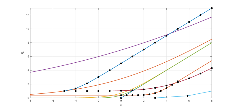
Figure 3.1: Some examples of both smooth and nonsmooth risk regularizers. Black dots highlight the respective corner points of nondifferentiability (some imperceptible).

The power of generalized semideviations is in the fact that they form a parametric family relative to the choice of the risk regularizer ${\cal R}$; different risk regularizers correspond to different rules for ranking the relative effect of both riskier (higher than the mean) and less risky (lower than the mean) events, corresponding to specific regions in the range of the cost. For more details, see Section 3, where we illustrate the versatility of generalized semideviations via additional examples, considering various specific choices for ${\cal R}$, with the well known upper-semideviation dispersion measure (Shapiro et al., 2014) being the prototypical representative of this class.

3.2 Mean-Semideviations: Definition, Existence & Structure

Utilizing the concept of generalized semideviations, we may now introduce the class of risk measures of central interest in this work, as follows.

Definition 5.

(Mean-Semideviation Risk Measures) Fix $p\in\left[1,\infty\right)$ and choose a risk regularizer ${\cal R}:\mathbb{R}\rightarrow\mathbb{R}$. The mean-semideviation of order $p$, induced by ${\cal R}$, or $MS_{p}^{{\cal R}}$, for short, is the real-valued risk measure defined, for $Z\in{\cal Z}_{q}$, as

$$\rho\left(Z\right)\equiv\rho_{p}^{{\cal R}}\left(Z;c\right) \triangleq\mathbb{E}\left\{Z\right\}+c\mathbb{D}_{p}^{{\cal R}}\left\{Z\right\},$$ (9)

where $c\geq 0$ constitutes a fixed penalty multiplier, and provided that all involved quantities are well defined and finite.

Next, we state and prove a small number of relatively simple results, related to the existence of mean-semideviation risk measures, introduced in Definition 5, as well as their functional structure. First, as it might be expected, we show that mean-semideviation risk measures of order $p$ may be naturally associated with costs which are also in ${\cal L}_{p}$ (i.e., choosing $p\equiv q$). Recall that, throughout the paper, $p$ is reserved for specifying the order of the mean-semideviation risk measure under consideration, whereas $q$ is related to the integrability of the respective cost.

Proposition 3.

(Compatibility of $p$’s and $q$’s) Fix $p\in\left[1,\infty\right)$, $c\geq 0$, and choose any risk regularizer ${\cal R}:\mathbb{R}\rightarrow\mathbb{R}$. Then, as long as $q\geq p$, the $MS_{p}^{{\cal R}}$ risk measure $\rho_{p}^{{\cal R}}\left(\cdot;c\right)$ is well-defined and finite, for every $Z\in{\cal Z}_{q}$.

Proof of Proposition 3.

Since $q\geq p\geq 1$, it is trivial that $Z\in{\cal Z}_{1}$, simply due to the inclusion ${\cal Z}_{1}\supset{\cal Z}_{2}\supset\ldots$, for any choice of $q$. Thus, the expectation of every $Z\in{\cal Z}_{q}$ exists and is finite, and what remains is to prove the result for the dispersion measure $\mathbb{D}_{p}^{{\cal R}}$.

For simplicity, let $q\equiv p$. Using the fact that $\mathbb{E}\left\{Z\right\}$ is finite, it is true that, for every $Z\in{\cal Z}_{p}$, the shifted cost $Z-\mathbb{E}\left\{Z\right\}$ is in ${\cal Z}_{p}$. It thus suffices to show that, for every $Z-\mathbb{E}\left\{Z\right\}\triangleq X\in{\cal Z}_{p}$, ${\cal R}\left(X\right)$ is in ${\cal Z}_{p}$, as well. Because the risk regularizer ${\cal R}$ is nonnegative (condition $\mathbf{S2}$), the integral $\mathbb{E}\left\{\left({\cal R}\left(X\right)\right)^{p}\right\}$ exists. Also, due to condition $\mathbf{S4}$ of Definition 3, it follows that, for every $x\geq 0$, ${\cal R}\left(x\right)\leq{\cal R}\left(0\right)+x,$ and since ${\cal R}$ is nondecreasing ($\mathbf{S3}$), it is true that ${\cal R}\left(x\right)\leq{\cal R}\left(0\right)+\left|x\right|$, for all $x\in\mathbb{R}$. Setting $x\equiv X$, this yields

$$0\leq{\cal R}\left(X\right)\leq{\cal R}\left(0\right)+\left|X\right|,$$ (10)

and since $X\in{\cal Z}_{p}$, ${\cal R}\left(0\right)+\left|X\right|\in{\cal Z}_{p}$, as well. Consequently, it is true that

$$\left(\mathbb{E}\left\{\left({\cal R}\left(X\right)\right)^{p}\right\}\right)^{1/p}\leq\left(\mathbb{E}\left\{\left({\cal R}\left(0\right)+\left|X\right|\right)^{p}\right\}\right)^{1/p}<+\infty,$$ (11)

showing that $\mathbb{D}_{p}^{{\cal R}}$ and, therefore, $\rho_{p}^{{\cal R}}\left(\cdot;c\right)$, are both well defined and finite, for every $Z\in{\cal Z}_{p}$.

Now, due to the inclusion ${\cal Z}_{1}\supset{\cal Z}_{2}\supset\ldots$, we know that, if $Z\in{\cal Z}_{q}$, for some $q\geq p$, then $Z\in{\cal Z}_{p}$, as well. Enough said. ∎

Hereafter, for the sake of generality, we will implicitly assume that $p$ and $q$ are compatible, so that existence and finiteness of the resulting risk measures considered is ensured. Of course, in actual applications, Proposition 3 may be directly invoked on a case-by-case basis, in order to select the order of the particular dispersion measure of choice, depending on the nature of the random cost, or a family of those, under study.

After characterizing existence and finiteness of mean-semideviation risk measures, as introduced in Definition 5, we focus on their structural properties, from a functional point of view. As the following result suggests, mean-semideviation risk measures are indeed convex-monotone under a standardized assumption on the penalty multiplier $c$.

Theorem 1.

(When are Mean-Semideviations Convex-Monotone?) Fix $p\in\left[1,\infty\right)$ and choose any risk regularizer ${\cal R}:\mathbb{R}\rightarrow\mathbb{R}$. Then, as long as $c\in\left[0,1\right]$, the $MS_{p}^{{\cal R}}$ risk measure $\rho_{p}^{{\cal R}}\left(\cdot;c\right)$ is convex-monotone; that is, it satisfies both conditions $\mathbf{R1}$ and $\mathbf{R2}$.

Proof of Theorem 1.

Let us start with verifying convexity ($\mathbf{R1}$). Since the expectation term of $\rho_{p}^{{\cal R}}\left(\cdot;c\right)$ is a linear functional on ${\cal Z}_{q}$, it will suffice to show that the generalized semideviation term $\mathbb{D}_{p}^{{\cal R}}$ is convex. Indeed, for every $Z_{1}\in{\cal Z}_{q}$, $Z_{2}\in{\cal Z}_{q}$ and every $\alpha\in\left[0,1\right]$, we may write

$$\mathbb{D}_{p}^{{\cal R}}\left\{\alpha Z_{1}+\left(1-\alpha\right)Z_{2}\right\} \equiv\left\|{\cal R}\left(\alpha Z_{1}+\left(1-\alpha\right)Z_{2}-\mathbb{E}\left\{\alpha Z_{1}+\left(1-\alpha\right)Z_{2}\right\}\right)\right\|_{{\cal L}_{p}}$$

$$\equiv\left\|{\cal R}\left(\alpha\left(Z_{1}-\mathbb{E}\left\{Z_{1}\right\}\right)+\left(1-\alpha\right)\left(Z_{2}-\mathbb{E}\left\{Z_{2}\right\}\right)\right)\right\|_{{\cal L}_{p}}$$

$$\leq\left\|\alpha{\cal R}\left(\left(Z_{1}-\mathbb{E}\left\{Z_{1}\right\}\right)\right)+\left(1-\alpha\right){\cal R}\left(Z_{2}-\mathbb{E}\left\{Z_{2}\right\}\right)\right\|_{{\cal L}_{p}}$$

$$\leq\alpha\left\|{\cal R}\left(\left(Z_{1}-\mathbb{E}\left\{Z_{1}\right\}\right)\right)\right\|_{{\cal L}_{p}}+\left(1-\alpha\right)\left\|{\cal R}\left(Z_{2}-\mathbb{E}\left\{Z_{2}\right\}\right)\right\|_{{\cal L}_{p}}$$

$$\equiv\alpha\mathbb{D}_{p}^{{\cal R}}\left\{Z_{1}\right\}+\left(1-\alpha\right)\mathbb{D}_{p}^{{\cal R}}\left\{Z_{2}\right\},$$ (12)

where the first inequality is true due to conditions $\mathbf{S1}$ (convexity) and $\mathbf{S2}$ (nonnegativity), and the second is due to the triangle (Minkowski) inequality. Thus, $\mathbb{D}_{p}^{{\cal R}}$ is a convex functional, which means that $\rho_{p}^{{\cal R}}\left(\cdot;c\right)$ is also convex on ${\cal Z}_{q}$. Note that the value of $c\geq 0$ is not crucial in order to show convexity of $\rho_{p}^{{\cal R}}\left(\cdot;c\right)$.

Let us now study monotonicity ($\mathbf{R2}$) of the risk measure $\rho_{p}^{{\cal R}}\left(\cdot;c\right)$. For every $Z_{1}\in{\cal Z}_{q}$ and $Z_{2}\in{\cal Z}_{q}$, such that $Z_{1}\left(\omega\right)\geq Z_{2}\left(\omega\right)$, for ${\cal P}$-almost all $\omega\in\Omega$, we have

$$\rho_{p}^{{\cal R}}\left(Z_{2};c\right) \equiv\mathbb{E}\left\{Z_{2}\right\}+c\left\|{\cal R}\left(Z_{2}-\mathbb{E}\left\{Z_{2}\right\}\right)\right\|_{{\cal L}_{p}}$$

$$\leq\mathbb{E}\left\{Z_{2}\right\}+c\left\|{\cal R}\left(Z_{1}-\mathbb{E}\left\{Z_{2}\right\}\right)\right\|_{{\cal L}_{p}}$$

$$\equiv\mathbb{E}\left\{Z_{2}\right\}+c\left\|{\cal R}\left(Z_{1}-\mathbb{E}\left\{Z_{1}\right\}+\mathbb{E}\left\{Z_{1}\right\}-\mathbb{E}\left\{Z_{2}\right\}\right)\right\|_{{\cal L}_{p}}$$

$$\leq\mathbb{E}\left\{Z_{2}\right\}+c\left\|{\cal R}\left(Z_{1}-\mathbb{E}\left\{Z_{1}\right\}\right)+\mathbb{E}\left\{Z_{1}\right\}-\mathbb{E}\left\{Z_{2}\right\}\right\|_{{\cal L}_{p}}$$

$$\leq\mathbb{E}\left\{Z_{2}\right\}+c\left(\mathbb{E}\left\{Z_{1}\right\}-\mathbb{E}\left\{Z_{2}\right\}\right)+c\left\|{\cal R}\left(Z_{1}-\mathbb{E}\left\{Z_{1}\right\}\right)\right\|_{{\cal L}_{p}},$$ (13)

where the first inequality is due to conditions $\mathbf{S2}$ (nonnegativity) and $\mathbf{S3}$ (monotonicity), the second is due to conditions $\mathbf{S2}$ (nonnegativity), $\mathbf{S4}$ (nonexpansiveness), as well as the fact that $\mathbb{E}\left\{Z_{1}\right\}\geq\mathbb{E}\left\{Z_{2}\right\}$, and the third is again due to the triangle inequality. From (13), we readily see that, as long as $c\in\left[0,1\right]$, we may further write

$$\rho_{p}^{{\cal R}}\left(Z_{2};c\right)\leq\mathbb{E}\left\{Z_{1}\right\}+c\left\|{\cal R}\left(Z_{1}-\mathbb{E}\left\{Z_{1}\right\}\right)\right\|_{{\cal L}_{p}}\equiv\rho_{p}^{{\cal R}}\left(Z_{1};c\right),$$ (14)

completing the proof of the theorem. ∎

We may now invoke Proposition 1, presented earlier, to immediately obtain the following key corollary. The proof is trivial and, thus, omitted.

Corollary 1.

(When is (4) Convex?) Fix $p\in\left[1,\infty\right)$ and choose any risk regularizer ${\cal R}:\mathbb{R}\rightarrow\mathbb{R}$. Then, as long as $c\in\left[0,1\right]$, the composite function $\phi^{\widetilde{F}}\left(\cdot\right)\equiv\rho_{p}^{{\cal R}}\left(F\left(\cdot,\boldsymbol{W}\right);c\right)\equiv\rho\left(F\left(\cdot,\boldsymbol{W}\right)\right)$ is convex on $\mathbb{R}^{N}$, and (4) constitutes a convex stochastic program.

Corollary 1 is an important result, because it shows that, for every mean-semideviation risk measure, or equivalently, for every risk regularizer of choice, problem (4) would be exactly solvable via, for instance, subgradient methods, if the function $\phi^{\widetilde{F}}$ was known in advance. This fact reinforces our hope that it might indeed be possible to solve (4) to optimality, utilizing some carefully designed stochastic search, or, more specifically, and based on the assumed subdifferentiability of $F\left(\cdot,\boldsymbol{W}\right)$, stochastic subgradient algorithm. Of course, such an algorithm should be designed to work under Assumptions 1 and 2, without the need for explicit knowledge of $F\left(\cdot,\boldsymbol{W}\right)$, or $\underline{\nabla}F\left(\cdot,\boldsymbol{W}\right)$.

Remark 2.

(Coherence?) We should mention that mean-semideviations are not coherent risk measures ((Shapiro et al., 2014), Section 6.3), since they do not satisfy the axiomatic property of positive homogeneity. This is simply due to the fact that, in general, one may find choices for ${\cal R}$ such that

$$\left\|{\cal R}\left(tZ-\mathbb{E}\left\{tZ\right\}\right)\right\|_{{\cal L}_{p}}\neq t\left\|{\cal R}\left(Z-\mathbb{E}\left\{Z\right\}\right)\right\|_{{\cal L}_{p}},$$ (15)

for some $t>0$ and $Z\in{\cal Z}_{q}$. Nevertheless, mean-semideviations may be readily shown to satisfy translation equivariance, although such property is not explicitly required in this work. As a result, except for being convex-monotone, mean-semideviations also belong to the class of convex risk measures (Föllmer and Schied, 2002; Shapiro et al., 2014). $\blacksquare$

3.3 Examples of Mean-Semideviation Models

Before moving on, it would be instructive to discuss some examples of mean-semideviations, highlighting the versatility of this particular class of risk measures. We start from simple, illustrative choices as far as the involved risk regularizer is concerned, and then we generalize.

3.3.1 Mean-Upper-Semideviations

The simplest, prototypical example of a mean-semideviation risk measure is the mean-upper-semide- viation of order $p$ ((Shapiro et al., 2014), Sections 6.2.2 & 6.3.2), which is constructed by choosing as risk regularizer the function

$${\cal R}\left(x\right)\triangleq\left(x\right)_{+}\triangleq\max\left\{x,0\right\},\quad x\in\mathbb{R},$$ (16)

yielding the risk measure

$$\rho\left(Z\right) \equiv\mathbb{E}\left\{Z\right\}+c\left(\mathbb{E}\left\{\left(\left(Z-\mathbb{E}\left\{Z\right\}\right)_{+}\right)^{p}\right\}\right)^{1/p}$$

$$\equiv\mathbb{E}\left\{Z\right\}+c\left\|\left(Z-\mathbb{E}\left\{Z\right\}\right)_{+}\right\|_{{\cal L}_{p}},$$ (17)

for $Z\in{\cal Z}_{q}$. Of course, in this case, it is trivial to show that ${\cal R}$ satisfies conditions $\mathbf{S1}$-$\mathbf{S4}$ of Definition 3. Recall that we have assumed that $q$ is appropriately chosen, such that $\rho$ is a well defined, real-valued functional on ${\cal Z}_{q}$.

3.3.2 Entropic Mean-Semideviations

Our second example is a generalization of the mean-upper-semideviation risk measure discussed in the previous example. Here, the risk regularizer ${\cal R}$ is chosen itself from a parametric family, as

$${\cal R}\left(x;t\right)\triangleq\dfrac{1}{t}\log\left(1+\exp\left(tx\right)\right),\quad\left(x,t\right)\in\mathbb{R}\times\mathbb{R}_{++},$$ (18)

where $t$ is a parameter, regulating the sharpness of the function at zero. It is trivial to verify conditions $\mathbf{S2}$ (nonnegativity) and $\mathbf{S3}$ (monotonicity). Also, for fixed $t$, the first derivative of ${\cal R}$ relative to $x$ is the logistic function

$$\dfrac{\partial{\cal R}}{\partial x}\left(x;t\right)\equiv\dfrac{\exp\left(tx\right)}{1+\exp\left(tx\right)}\in\left(0,1\right),\quad\forall x\in\mathbb{R},$$ (19)

showing that ${\cal R}$ is a contraction mapping, immediately verifying condition $\mathbf{S4}$ (nonexpansiveness), via Proposition 2. Likewise, the second derivative of ${\cal R}$ is given by

$$\dfrac{\partial^{2}{\cal R}}{\partial x^{2}}\left(x;t\right)\equiv\dfrac{t\exp\left(tx\right)}{\left(1+\exp\left(tx\right)\right)^{2}}>0,\quad\forall x\in\mathbb{R},$$ (20)

and, thus, $\mathbf{S1}$ (convexity) is readily verified, as well. Hence, ${\cal R}$ is a valid risk regularizer. Alternatively and to illustrate the procedure, we may verify condition $\mathbf{S4}$ directly; for fixed $t>0$, for every $\alpha\geq 0$ and for every $x\in\mathbb{R}$, we may write

$${\cal R}\left(x+a;t\right) \equiv\dfrac{1}{t}\log\left(1+\exp\left(t\left(x+\alpha\right)\right)\right)$$

$$\equiv\dfrac{1}{t}\log\left(\dfrac{1}{\exp\left(t\alpha\right)}+\exp\left(tx\right)\right)+\alpha$$

$$\leq\dfrac{1}{t}\log\left(1+\exp\left(tx\right)\right)+\alpha$$

$$\equiv{\cal R}\left(x;t\right)+\alpha,$$ (21)

where the inequality is due to the fact that $t\alpha\geq 0$. It is also easy to see that, for every $x\in\mathbb{R}$, ${\cal R}\left(x;t\right)\underset{t\rightarrow\infty}{\longrightarrow}\left(x\right)_{+}$, showing that ${\cal R}\left(\cdot;t\right)$ constitutes a smooth approximation to the risk regularizer of the mean-upper-semideviation risk measure discussed previously.

The resulting risk measure is called an entropic mean-semideviation of order $p$, and may be expressed as

$$\rho\left(Z\right)\equiv\mathbb{E}\left\{Z\right\}+\dfrac{c}{t}\left\|\log\left(1+\exp\left(t\left(Z-\mathbb{E}\left\{Z\right\}\right)\right)\right)\right\|_{{\cal L}_{p}},$$ (22)

for $Z\in{\cal Z}_{q}$. For obvious reasons, this risk measure may be considered a soft version of the mean-upper-semideviation risk measure.

3.3.3 CDF-Antiderivative (CDFA) Mean-Semideviations

We now show that, in fact, both previously presented examples are special cases of a much more general approach, which may be utilized for the construction of risk regularizers. To this end, let $Y:\Omega\rightarrow\mathbb{R}$ be a random variable in ${\cal Z}_{1}$, with cumulative distribution function (cdf) $F_{Y}$. Consider the choice

$${\cal R}\left(x\right)\triangleq\int_{-\infty}^{x}F_{Y}\left(y\right)\textrm{d}y,\quad x\in\mathbb{R},$$ (23)

where, because $F_{Y}$ is a nonnegative Borel measurable function, the involved integration is always well-defined (might be $+\infty$, though), in the sense of Lebesgue. The particular antiderivative of the cdf $F_{Y}$, as defined in (23), constitutes a very important quantity in the theory of stochastic dominance; see, for instance, related articles (Ogryczak and Ruszczyński, 1999) and (Ogryczak and Ruszczyński, 2002) for definition and insights. In particular, via Fubini’s Theorem (Theorem 2.6.6 in (Ash and Doléans-Dade, 2000)), ${\cal R}$ may be easily shown to admit the alternative integral representation

$${\cal R}\left(x\right)\equiv\mathbb{E}\left\{\left(x-Y\right)_{+}\right\},\quad\forall x\in\mathbb{R}.$$ (24)

Exploiting the assumption that $Y\in{\cal Z}_{1}$, it follows that ${\cal R}\left(x\right)<+\infty$, for every $x\in\mathbb{R}$. Also, from (24), it is trivial to see that, because of the structure of the function $\left(\cdot\right)_{+}$, ${\cal R}$ is convex ($\mathbf{S1}$), nonnegative ($\mathbf{S2}$) and nondecreasing ($\mathbf{S3}$) on $\mathbb{R}$. Nonexpansiveness ($\mathbf{S4}$) may also be readily verified.

Consequently, ${\cal R}$ is a valid risk regularizer, and the resulting risk measure, called a CDF-Antiderivative (CDFA) mean-semideviation, may be expressed in various forms as

$$\rho\left(Z\right) \equiv\mathbb{E}\left\{Z\right\}+c\left\|\int_{-\infty}^{Z-\mathbb{E}\left\{Z\right\}}F_{Y}\left(y\right)\textrm{d}y\right\|_{{\cal L}_{p}}$$

$$\equiv\mathbb{E}\left\{Z\right\}+c\left\|\left.\mathbb{E}\left\{\left(x-Y\right)_{+}\right\}\right|_{x\equiv Z-\mathbb{E}\left\{Z\right\}}\right\|_{{\cal L}_{p}}$$

$$\equiv\mathbb{E}\left\{Z\right\}+c\left\|\int_{\mathbb{R}}\left(\left[Z-\mathbb{E}\left\{Z\right\}\right]-y\right)_{+}\textrm{d}{\cal P}_{Y}\left(y\right)\right\|_{{\cal L}_{p}}$$

$$\equiv\mathbb{E}\left\{Z\right\}+c\left\|\mathbb{E}\left\{\left.\left(\left[Z-\mathbb{E}\left\{Z\right\}\right]-Y\right)_{+}\right|Z\right\}\right\|_{{\cal L}_{p}},$$ (25)

for $Z\in{\cal Z}_{q}$, where $Y$ can be arbitrarily taken to be independent of $Z$ and ${\cal P}_{Y}$ denotes the Borel pushforward of $Y$.

We may now verify that both mean-upper-semideviation and entropic mean-semideviation risk measures discussed above are special cases of CDFA mean-semideviations. In mean-upper-semidevi- ations, the respective risk regularizer is an antiderivative (taken piecewise) of the cdf corresponding to the Dirac measure at zero. In entropic mean-semideviations, the respective risk regularizer is an antiderivative of (19) (by monotone convergence and via a sequential argument), which is the cdf of a zero-mean element in ${\cal Z}_{1}$. In both cases, the antiderivatives involved are of the form of (23).

3.3.3.1 Special Case: Gaussian Antiderivative (GA) Mean-Semideviations

An interesting subclass of CDFA mean-semideviations is the one resulting from taking antiderivatives of the cdf of a standard Gaussian random variable $Y\sim{\cal N}\left(0,1\right)$. In this case, the simplest possible risk regularizer may be constructed as

$${\cal R}\left(x\right)\triangleq\int_{-\infty}^{x}\varPhi\left(y\right)\textrm{d}y\equiv x\varPhi\left(x\right)+\varphi\left(x\right),\quad x\in\mathbb{R},$$ (26)

where $\varPhi:\mathbb{R}\rightarrow\left[0,1\right]$ and $\varphi:\mathbb{R}\rightarrow\mathbb{R}$ denote the standard Gaussian cdf and density, respectively. This particular antiderivative of $\varPhi$ appears naturally in standard treatments of the so-called ranking-&-selection, or best arm identification problem and, more specifically, in lookahead selection policies, such as the Knowledge Gradient and the Expected Improvement (Frazier et al., 2008; Ryzhov, 2016).

The resulting mean-semideviation risk measure is called a Gaussian Antiderivative (GA) mean-semideviation of order $p$, and may be expressed as

$$\rho\left(Z\right)\equiv\mathbb{E}\left\{Z\right\}+c\left\|\left(Z-\mathbb{E}\left\{Z\right\}\right)\varPhi\left(Z-\mathbb{E}\left\{Z\right\}\right)+\varphi\left(Z-\mathbb{E}\left\{Z\right\}\right)\right\|_{{\cal L}_{p}},$$ (27)

for $Z\in{\cal Z}_{q}$. Of course, as it happens for all mean semideviations, the functional $\rho$, as defined in (27), is a convex risk measure for every $c\geq 0$, and a convex-monotone risk measure, if $c\in\left[0,1\right]$.

3.4 A Complete Characterization of Mean-Semideviations

As a result of the discussion in Section 3.3.3 above, it follows that risk regularizers may be formed by taking antiderivatives of the cdf of any integrable random variable of choice, resulting in a vast variety of mean-semideviation risk measures, all sharing a common favorable structure.

Here, we show that if we start from a given risk regularizer ${\cal R}$, the converse statement is also true. In this respect, we state and prove the following important result.

Theorem 2.

(CDF-Based Representation of Risk Regularizers) Let $Y:\Omega\rightarrow\mathbb{R}$ be a random variable, such that, for every $x\in\mathbb{R}$, $\mathbb{E}\left\{\left(x-Y\right)_{+}\right\}<+\infty$, and let $F_{Y}:\mathbb{R}\rightarrow\left[0,1\right]$ denote its cdf. Then, for any fixed $0\leq C_{S}\leq 1$ and $C_{I}\geq 0$, the function ${\cal R}:\mathbb{R}\rightarrow\mathbb{R}$ defined as

$${\cal R}\left(x\right)\triangleq C_{S}\int_{-\infty}^{x}F_{Y}\left(y\right)\textrm{d}y+C_{I},\quad\forall x\in\mathbb{R},$$ (28)

is a valid risk regularizer, where integration may be interpreted either in the improper Riemann sense (for computation), or in the standard sense of Lebesgue (for derivation).

Conversely, let ${\cal R}:\mathbb{R}\rightarrow\mathbb{R}$ be any risk regularizer. Then, there exist some random variable $Y:\Omega\rightarrow\mathbb{R}$, satisfying $\mathbb{E}\left\{\left(x-Y\right)_{+}\right\}<+\infty$, for all $x\in\mathbb{R}$, with cdf $F_{Y}:\mathbb{R}\rightarrow\left[0,1\right]$, and constants $0\leq C_{S}\leq 1$ and $C_{I}\geq 0$, such that, for every $x\in\mathbb{R}$, the representation (28) is valid. In particular, if ${\cal R}^{\prime}_{+}:\mathbb{R}\rightarrow\mathbb{R}$ denotes the right derivative of ${\cal R}$, it is always true that $C_{S}\equiv\sup_{x\in\mathbb{R}}{\cal R}^{\prime}_{+}\left(x\right)$, $C_{I}\equiv\inf_{x\in\mathbb{R}}{\cal R}\left(x\right)$, and, as long as ${\cal R}$ is nonconstant, it holds that $C_{S}\neq 0$, and $F_{Y}$ is given by $F_{Y}\left(x\right)\equiv C_{S}^{-1}{\cal R}^{\prime}_{+}\left(x\right),$ for all $x\in\mathbb{R}$.

Proof of Theorem 2.

See Section 7.1 (Appendix). ∎

Theorem 2 is important for two main reasons, the first being related to the forward statement, and the second to the converse. On the one hand, Theorem 2 provides us with the clean, very versatile and analytically friendly integral formula (28) for constructing risk regularizers of various shapes and types. On the other hand, it informs us that, necessarily, any risk regularizer can be expressed in the form of (28) and, as a result, all possible risk regularizers may be constructed utilizing (28), each time for some suitably chosen cdf. Therefore, risk regularizers are completely characterized by the cdf-based representation of Theorem 2.

Of course, every risk regularizer induces a unique mean-semideviation risk measure. But also notice that, trivially, every mean-semideviation risk measure corresponds to a uniquely specified risk regularizer (as a functional, or when all costs in the corresponding ${\cal L}_{p}$-space ${\cal Z}_{p}$ -the largest such space, for the smallest possible $q$- are considered). Therefore, Theorem 2 provides a complete characterization of the whole class of mean-semideviation risk measures. In particular, Theorem 2 implies that the class of all mean-semideviation risk measures is almost in one-to-one correspondence with the class of cdfs of all integrable $\mathbb{R}$-valued random elements. The “almost” in the preceding statement is due to the presence of constants $C_{S}$ and $C_{I}$ in Theorem 2, and that actually slightly less is required than (absolute) integrability of the involved random variable $Y$.

3.5 Practical Illustration of Mean-Semideviation Models

We conclude this section by briefly outlining the relevance of mean-semideviation models in applications, also putting our proposed risk regularizers in context. More specifically, we consider a chance-constrained version of the prototypical, single-product newsvendor problem (see, for instance, Chapter 1 in (Shapiro et al., 2014)), upon which we are based in order to formulate a doubly risk-averse newsvendor problem, which jointly controls both unmet demand and holding costs. We also explicitly demonstrate how the respective risk regularizer may be potentially designed, based on the characteristics of the particular problem under consideration.

Although the single-product newsvendor problem (and its variations) indeed constitutes a one-dimensional, toy example, it provides insights and highlights some important features of the mean-semideviation risk measures advocated herein. Additionally, the simplicity of such a problem facilitates numerical solution, and enables us to present some numerical results, verifying the effectiveness of the proposed mean-semideviation risk measures experimentally, as well.

3.5.1 A Chance-Constrained Single-Product NewsVendor

Suppose that a newsvendor is interested in optimally producing newspapers for an uncertain market, so that they minimize the cost incurred by actual production and by not meeting market demand, while respecting their holding capacity, or a predefined holding cost target. Let $K^{P}>0$, $K^{U}>0$ and $K^{H}>0$ be known constants, standing for the production, unmet demand and holding costs per production unit. Also let $W:\Omega\rightarrow\mathbb{R}_{+}$ be the random market demand, a random variable with cdf $F_{W}:\mathbb{R}\rightarrow\left[0,1\right]$, for simplicity assumed to be absolutely continuous relative to the Lebesgue measure on $\left(\mathbb{R},\mathscr{B}\left(\mathbb{R}\right)\right)$. Since the market is uncertain, the newsvendor resorts to stochastically deciding their production plan by solving the chance-constrained program

$$\begin{array}[]{rl}\underset{x}{\mathrm{minimize}}&K^{P}x+\mathbb{E}\left\{K^{U}\left(W-x\right)_{+}\right\}\\ \mathrm{subject\,to}&{\cal P}\left(K^{H}\left(x-W\right)_{+}>h\right)\leq\alpha\\ &x\geq 0\end{array},$$ (29)

where, also for simplicity, we assume that the decision variable is real-valued, and where $0\leq\alpha\leq 1$ constitutes the newsvendor’s tolerance in the event that their holding cost $K^{H}\left(x-W\right)_{+}$ will exceed a prescribed threshold $h\geq 0$. Both $\alpha$ and $h$ are fixed design parameters decided by the newsvendor beforehand. Chance-constrained newsvendor problems similar to (29) have been previously considered in the literature; see, for instance, the related article (Zhang et al., 2009). Here, an important detail is that, despite the probabilistic constraint, problem (29) is risk-neutral as far as treatment of unmet demand is concerned. This is because only the expectation of the cost of not meeting the demand, corresponding to $K^{U}\left(W-x\right)_{+}$, is considered in the objective.

Problem (29) exhibits some interesting features and may be significantly simplified, as follows. First, we may observe that, for every fixed choice of $h\geq 0$,

$${\cal P}\left(K^{H}\left(x-W\right)_{+}>h\right) ={\cal P}\left(K^{H}\left(x-W\right)>h\right)$$

$$\equiv{\cal P}\left(W<x-\dfrac{h}{K^{H}}\right)$$

$$\equiv F_{W}\left(x-\dfrac{h}{K^{H}}\right),\quad\forall x\in\mathbb{R}.$$ (30)

Consequently, it is true that

$${\cal P}\left(K^{H}\left(x-W\right)_{+}>h\right)\leq\alpha \iff F_{W}\left(x-\dfrac{h}{K^{H}}\right)\leq\alpha$$

$$\iff x\leq F_{W}^{-1}\left(\text{$\alpha$}\right)+\dfrac{h}{K^{H}}$$ (31)

$$\iff{\cal P}\left(W<x\right)\leq F_{W}\left(F_{W}^{-1}\left(\text{$\alpha$}\right)+\dfrac{h}{K^{H}}\right),$$ (32)

where, due to $F_{W}$ being continuous, the pseudo-inverse or quantile function $F_{W}^{-1}:\left[0,1\right]\rightarrow\mathbb{R}_{+}$ is defined as

$$F_{W}^{-1}\left(\alpha\right)\triangleq\inf\left\{x\in\mathbb{R}\left|F_{W}\left(x\right)\geq\alpha\right.\right\}\equiv\sup\left\{x\in\mathbb{R}\left|F_{W}\left(x\right)\leq\alpha\right.\right\}.$$ (33)

Thus, problem (29) is convex and may be reformulated as

$$\begin{array}[]{rl}\underset{x}{\mathrm{minimize}}&K^{P}x+\mathbb{E}\left\{K^{U}\left(W-x\right)_{+}\right\}\\ \mathrm{subject\,to}&x\in\left[0,F_{W}^{-1}\left(\text{$\alpha$}\right)+\dfrac{h}{K^{H}}\right]\end{array}.$$ (34)

Hereafter, without loss of generality, we may assume that $\alpha$ and $h$ are chosen such that $F_{W}^{-1}\left(\text{$\alpha$}\right)+h/K^{H}>0$. Otherwise, the problem is trivially solved at $x^{*}\equiv 0$. To be fully compatible with the generic notation utilized in this paper, we may also define $F\left(\cdot,\bullet\right)\triangleq K^{P}\left(\cdot\right)+K^{U}\left(\left(\bullet\right)-\left(\cdot\right)\right)_{+},$ and ${\cal X}\triangleq\left[0,F_{W}^{-1}\left(\text{$\alpha$}\right)+h/K^{H}\right]$.

Next, let us consider the derivative of the objective of (34), relative to $x$. We have

$$\nabla\mathbb{E}\left\{F\left(x,W\right)\right\}=K^{P}-K^{U}{\cal P}\left(W\geq x\right),\quad\forall x\in{\cal X}.$$ (35)

Hence, unless $K^{U}>K^{P}$, it readily follows that, for every $x\in{\cal X}$, $\nabla\mathbb{E}\left\{F\left(x,W\right)\right\}\geq 0$, again implying that the choice $x^{*}\equiv 0$ constitutes a solution of (34); in other words, producing nothing is always optimal whenever $K^{U}\leq K^{P}$. On the other hand, it is apparently true that $\nabla\mathbb{E}\left\{F\left(x,W\right)\right\}<0$, for all $x\in{\cal X}$, if and only if

$$K^{P}-K^{U}\left(1-{\cal P}\left(W<x\right)\right)<0,\quad\forall x\in{\cal X},$$ (36)

implying that the condition

$$K^{P}-K^{U}\left(1-F_{W}\left(F_{W}^{-1}\left(\text{$\alpha$}\right)+\dfrac{h}{K^{H}}\right)\right)<0$$ (37)

is sufficient to ensure negativity of $\nabla\mathbb{E}\left\{F\left(x,W\right)\right\}$ everywhere within the feasible set ${\cal X}$ (where (32) is always satisfied), in which case the choice $x^{*}\equiv F_{W}^{-1}\left(\text{$\alpha$}\right)+h/K^{H}$ constitutes the optimal production level. Putting it altogether, whenever

$$F_{W}\left(F_{W}^{-1}\left(\text{$\alpha$}\right)+\dfrac{h}{K^{H}}\right)>0,$$ (38)

the condition

$$K^{U}\left(1-F_{W}\left(F_{W}^{-1}\left(\text{$\alpha$}\right)+\dfrac{h}{K^{H}}\right)\right)\leq K^{P}<K^{U}$$ (39)

ensures that problem (29) admits nontrivial solutions, thus being of technical interest.

Problem (29) may be solved in closed form. Indeed, either by considering the Karush-Kuhn-Tucker (KKT) conditions for problem (29) (for a constraint qualification, we may observe that Slater’s condition is satisfied trivially whenever $F_{W}^{-1}\left(\text{$\alpha$}\right)+h/K^{H}>0$), or by looking at its geometric structure directly, it may be easily shown that its optimal solution may be expressed analytically as

$$x^{*}=\begin{cases}0,&\text{if }K^{U}\leq K^{P}\\ \min\left\{F_{W}^{-1}\left(\dfrac{K^{U}-K^{P}}{K^{U}}\right),F_{W}^{-1}\left(\text{$\alpha$}\right)+\dfrac{h}{K^{H}}\right\},&\text{if }K^{U}>K^{P}\end{cases},$$ (40)

representing the newsvendor’s optimal decision in regard to the quantity of newspapers they would have to plan for, before the random market demand $W$ is revealed.

Remark 3.

Problems of the type of (29) are meaningful in various settings; specifically, they are most suitable when holding is operationally more important than unmet demand. For instance, it might be the case that the event where holding exceeds some threshold might have severe economic consequences, while not meeting the demand might be tolerable, although undesirable.

Additionally and perhaps more importantly, we should mention that a chance-constrained approach such as that adopted in (29) allows to efficiently blend economic with physical quantities in a single stochastic program. This is simply due to the fact that by defining a quantity $\widetilde{h}\triangleq h/K^{H}\geq 0$, the probabilistic constraint of (29) may be written as

$${\cal P}\left(\left(x-W\right)_{+}>\widetilde{h}\right)\leq\alpha,$$ (41)

implying that, if we want to, we may directly choose $\widetilde{h}$ as a probabilistic upper bound directly on the excess production $\left(x-W\right)_{+}$.

The modification above can be very useful if we are willing to consider the problem

$$\begin{array}[]{rl}\underset{x}{\mathrm{minimize}}&K^{P}x+\mathbb{E}\left\{K^{H}\left(x-W\right)_{+}\right\}\\ \mathrm{subject\,to}&{\cal P}\left(K^{U}\left(W-x\right)_{+}>u\right)\leq\alpha\\ &x\geq 0\end{array},$$ (42)

which constitutes a dual version of the initial newsvendor problem (29) resulting by interchanging the two respective stochastic costs and where, similarly to (29), $u\geq 0$ is a prescribed threshold. In this case, unmet demand is operationally more important than holding, by choice. Of course, problem (42) is structurally very similar to (29), and can be analyzed via almost the same procedure as above. By defining $\widetilde{u}\triangleq u/K^{U}\geq 0$, problem (42) may be reformulated as

$$\begin{array}[]{rl}\underset{x}{\mathrm{minimize}}&K^{P}x+\mathbb{E}\left\{K^{H}\left(x-W\right)_{+}\right\}\\ \mathrm{subject\,to}&{\cal P}\left(\left(W-x\right)_{+}>\widetilde{u}\right)\leq\alpha\\ &x\geq 0\end{array},$$ (43)

where $\widetilde{u}$ can now be preselected directly. We may readily observe that the objective of (43) constitutes an economic quantity (a cost), whereas the probabilistic constraint is placed on the unmet demand itself, which, of course, is a physical quantity. This modification can be extremely useful in a more realistic scenario, since in many practical cases the unit cost of unmet demand, $K^{U}$, is either completely unknown, or extremely difficult to estimate based on experience. $\blacksquare$

3.5.2 A Doubly Risk-Averse Single-Product NewsVendor

Suppose now that, due to high variability of the market demand, the newsvendor realizes that minimizing their unmet demand cost in expectation does not constitute a very meaningful objective. Thus, the newsvendor would like to decide on their newspaper production size by explicitly accounting for market variability in their model and, because they are reasonable, they are willing to settle with a potentially slightly higher expected monetary penalty for not meeting market demand. In effect, the newsvendor is interested in making their decision by additionally considering the risk incurred due to stochastic variability in the resulting unmet demand, the latter realized when market demand is revealed. In other words, the newsvendor would like to come up with a meaningful doubly risk-averse version of the original, chance-constrained problem (29).

The newsvendor may think as follows. For every fixed and feasible production decision $x\in{\cal X}$, if the noisy unmet demand $\left(W-x\right)_{+}$ is smaller than $\mathbb{E}\left\{\left(W-x\right)_{+}\right\}$, which is the newsvendor’s expectation, then there is no risk incurred, since the newsvendor has been prepared for and has agreed to settle with a cost of unmet demand equal to $\mathbb{E}\left\{K^{U}\left(W-x\right)_{+}\right\}$. In an actual production scenario, $\mathbb{E}\left\{\left(W-x\right)_{+}\right\}$ might correspond to a small quantity of newspapers which are not actually produced, but for which resources have been allocated beforehand, to compensate for the case $W$ is greater than $x$, but not too much. In other words, we might think about the quantity $\mathbb{E}\left\{\left(W-x\right)_{+}\right\}$ as a risk-free, first-level safety stock.

Positive risk is incurred whenever $\left(W-x\right)_{+}>\mathbb{E}\left\{\left(W-x\right)_{+}\right\}$. However, the newsvendor realizes that not all values of the central deviation

$$CD\left(x,W\right)\triangleq\left(W-x\right)_{+}-\mathbb{E}\left\{\left(W-x\right)_{+}\right\}$$ (44)

are of equal importance, or equal severity. In other words, the newsvendor’s risk is variable relative to the value of $CD\left(x,W\right)$. Under the reasonable assumption that positive risk should be increasing as a function of the deviation $CD\left(x,W\right)$, the newsvendor’s realization translates naturally into a variable and increasing rate of change of the risk, relative to the values of the deviation. In particular, whenever $CD\left(x,W\right)>0$, the newsvendor identifies the following risk-incurring regions of increasing severity:

1. $CD\left(x,W\right)\in\left(0,t_{1}>0\right]$. In this case, unmet demand is higher than what the newsvendor expects, but its deviation from their expectation is no higher than a fixed threshold $t_{1}$. The value $\mathbb{E}\left\{\left(W-x\right)_{+}\right\}+t_{1}$ corresponds to the maximum partially unplanned or unexpected production quantity that the newsvendor may be able to produce today, potentially using presently unallocated resources. We might think about the threshold $t_{1}$ as a risk-incurring, second-level safety stock.

2. $CD\left(x,W\right)\in\left(t_{1},t_{2}>t_{1}\right]$. Here, the deviation of the unmet demand from the newsvendor’s expectation is exceeds $t_{1}$, but is no higher than another fixed threshold $t_{2}$. The value $t_{2}-t_{1}$ corresponds to the maximum quantity of newspapers that the newsvendor cannot produce in-house today, but may ask a nearby vendor to produce for them. Of course, such events should incur higher and more severely increasing risk, since the newsvendor essentially borrows resources from the nearby vendor. We might call $t_{2}$ as the borrowing threshold.

3. $CD\left(x,W\right)\in\left(t_{2},\infty\right)$. This constitutes an event of “total disaster,” in which it is impossible for the newsvendor to compensate for unmet market demand. When $CD\left(x,W\right)>t_{2}$, unmet demand is so high that it cannot be met even if the newsvendor borrows the maximum amount of resources from some nearby newsvendor. This might have severe consequences for the newsvendor, since they either might be in debt, or even lose their professional credibility, or both.

Although potentially simplified, a narrative such as the above is reasonable and quite realistic. Of course, what is important for us in the context of this paper, is the fact that the characteristics of the relatively complex risk dynamics discussed above can be succinctly captured by an appropriately shaped risk regularizer, as proposed and analyzed herein. As a simplest example, we may define a piecewise linear risk regularizer ${\cal R}^{nv}:\mathbb{R}\rightarrow\mathbb{R}$ as

$${\cal R}^{nv}\left(x\right)\triangleq\begin{cases}0,&\text{if }x\leq 0\\ \psi_{1}x,&\text{if }0<x\leq K^{U}t_{1}\\ \psi_{2}x+\left(\psi_{1}-\psi_{2}\right)K^{U}t_{1},&\text{if }K^{U}t_{1}<x\leq K^{U}t_{2}\\ x+\left(\psi_{2}-1\right)K^{U}t_{2}+\left(\psi_{1}-\psi_{2}\right)K^{U}t_{1},&\text{if }x>K^{U}t_{2}\end{cases},$$ (45)

where the risk slopes $\psi_{1}\geq 0$ and $\psi_{2}\geq 0$ are chosen such that $\psi_{1}\leq\psi_{2}\leq 1$. Of course, ${\cal R}$ may be rewritten as

$${\cal R}^{nv}\left(x\right) \equiv\psi_{1}x\mathds{1}_{\left[0,K^{U}t_{1}\right)}\left(x\right)+\left(\psi_{2}x+\left(\psi_{1}-\psi_{2}\right)K^{U}t_{1}\right)\mathds{1}_{\left[K^{U}t_{1},K^{U}t_{2}\right)}\left(x\right)$$

$$\quad\quad+\left(x+\left(\psi_{2}-1\right)K^{U}t_{2}+\left(\psi_{1}-\psi_{2}\right)K^{U}t_{1}\right)\mathds{1}_{\left[K^{U}t_{2},\infty\right)}\left(x\right),$$ (46)

for all $x\in\mathbb{R}$, and may be conveniently thought as a generalization of the positive part function of the upper-semideviation dispersion measure. Equivalently, the risk regularizer ${\cal R}^{nv}$ may be defined as an antiderivative of the cdf $F_{Y}^{nv}:\mathbb{R}\rightarrow\left[0,1\right]$ corresponding to some random variable $Y:\Omega\rightarrow\mathbb{R}$ in ${\cal Z}_{\infty}$, and defined as

$$F_{Y}^{nv}\left(x\right)\triangleq\psi_{1}\mathds{1}_{\left[0,K^{U}t_{1}\right)}\left(x\right)+\psi_{2}\mathds{1}_{\left[K^{U}t_{1},K^{U}t_{2}\right)}\left(x\right)+\mathds{1}_{\left[K^{U}t_{2},\infty\right)}\left(x\right),\quad x\in\mathbb{R},$$ (47)

as suggested by Theorem 2. The cdf $F_{Y}^{nv}$ expresses precisely the rate of increase of the risk incurred at each $x\in\mathbb{R}$, where $x$ may be thought of as the central deviation of the quantity whose risk is assessed by the risk regularizer ${\cal R}^{nv}$; in the newsvendor’s case, this quantity should be the noisy economic consequence due to unmet demand, i.e., $K^{U}\left(W-x\right)_{+}$, also justifying the multiplication of thresholds $t_{1}$ and $t_{2}$ with the unit cost $K^{U}$ in (45). Essentially, $F_{Y}^{nv}$ admits an intuitive interpretation, and can be utilized in order to actually design ${\cal R}^{nv}$, as well; also see Theorem 2.

If the newsvendor chooses the risk slopes $\psi_{1}$ and $\psi_{2}$ such that $\psi_{1}<\psi_{2}<1$ (only they know how set specific appropriate values), the quantity ${\cal R}^{nv}\left(K^{U}CD\left(x,W\right)\right)$ (for a fixed and feasible $x\in{\cal X}$) captures the dynamic behavior of the risk incurred by the central deviation $CD\left(x,W\right)$ when taking different values in $\mathbb{R}_{+}$, as described above. Essentially, ${\cal R}^{nv}$ may be regarded as a nonlinear weighting function acting on $K^{U}CD\left(x,W\right)$, whose shape has been carefully designed in order to reflect the newsvendor’s particular context.

Now, the newsvendor is interested in utilizing ${\cal R}^{nv}\left(K^{U}CD\left(\cdot,W\right)\right)$ for decision making purposes. Since, for each $x\in{\cal X}$, ${\cal R}^{nv}\left(K^{U}CD\left(\cdot,W\right)\right)$ depends pointwise on the random market demand $W$, which is unobservable when the newsvendor decides their production plan, it is most reasonable to consider the ${\cal L}_{p}$-norm of ${\cal R}^{nv}\left(K^{U}CD\left(\cdot,W\right)\right)$, for some prespecified $p\in\left[1,\infty\right)$, as a measure of magnitude. Of course, lower values for such deterministic term are preferred. In order to effectively manage their risk during decision making, the newsvendor proceeds by adding the ${\cal L}_{p}$-norm of ${\cal R}^{nv}\left(K^{U}CD\left(\cdot,W\right)\right)$ as a penalty term to their original, risk-neutral objective, leading to the risk-averse stochastic program

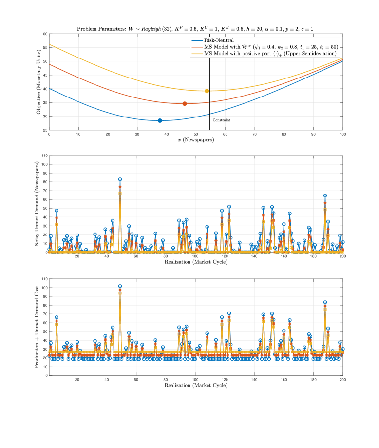
Figure 3.2: Top: Objective as a function of the production decision, for each of the following three cases: Risk neutral (problem (29)), risk-averse of the form (50), and risk-averse of the form (50), but with ${\cal R}^{nv}$ being replaced by $\left(\cdot\right)_{+}$. Middle: Unmet demand realizations as a function of the market cycle, for each of the three cases. Bottom: Combined monetary cost of production plus unmet demand realizations as a function of the market cycle, for each of the three cases.

$$\begin{array}[]{rl}\underset{x}{\mathrm{minimize}}&K^{P}x+\mathbb{E}\left\{K^{U}\left(W-x\right)_{+}\right\}+c\left\|{\cal R}^{nv}\left(K^{U}\left(W-x\right)_{+}-\mathbb{E}\left\{K^{U}\left(W-x\right)_{+}\right\}\right)\right\|_{{\cal L}_{p}}\\ \mathrm{subject\,to}&{\cal P}\left(K^{H}\left(x-W\right)_{+}>h\right)\leq\alpha\\ &x\geq 0\end{array},$$ (48)

where, in general, $c\geq 0$ denotes the corresponding penalty tradeoff multiplier. It is then easy to see that the objective of problem (48) constitutes a mean-semideviation model. Indeed, by equivalently rewriting ${\cal R}^{nv}\left(K^{U}CD\left(\cdot,W\right)\right)$ as

$${\cal R}^{nv}\left(K^{U}CD\left(x,W\right)\right) \equiv{\cal R}^{nv}\left(K^{P}x+K^{U}\left(W-x\right)_{+}-\mathbb{E}\left\{K^{P}x+K^{U}\left(W-x\right)_{+}\right\}\right)$$

$$\equiv{\cal R}^{nv}\left(F\left(x,W\right)-\mathbb{E}\left\{F\left(x,W\right)\right\}\right),\quad\forall x\in{\cal X},$$ (49)

problem (48) may be equivalently restated as

$$\begin{array}[]{rl}\underset{x}{\mathrm{minimize}}&\mathbb{E}\left\{F\left(x,W\right)\right\}+c\left\|{\cal R}^{nv}\left(F\left(x,W\right)-\mathbb{E}\left\{F\left(x,W\right)\right\}\right)\right\|_{{\cal L}_{p}}\\ \mathrm{subject\,to}&x\in{\cal X}\end{array}.$$ (50)

Apparently, the objective of problem (50) is a mean-semideviation risk measure. Of course, whenever $c\in\left[0,1\right]$, (50) (and thus, (48), as well) constitutes a convex, risk-averse stochastic program, precisely of the form considered in this paper.

To empirically demonstrate the effectiveness of the risk-averse newsvendor problem (50), we have conducted numerical simulations concerning the following three cases: Initial problem (29) (risk neutral), risk-averse problem (50), and risk-averse of the form (50), but with ${\cal R}^{nv}$ being replaced by $\left(\cdot\right)_{+}$, resulting to the mean-upper-semideviation risk measure. In all simulations, the random market demand $W$ follows a Rayleigh distribution, and all necessary expectations present in each objective have been approximated utilizing $5\cdot 10^{6}$ demand realizations, sampled independently. The precise values for the scale of the aforementioned distribution and for all the rest of parameters involved in problem (50) are shown in the title of Fig. 3.2 (top), respectively.

From Fig. 3.2 (top), we observe that the optimal production decision obtained by solving (50) is distinctly different from the respective solutions obtained by solving both the risk neutral problem (29), and the risk-averse problem employing the mean-upper-semideviation risk measure (all optimal solutions are represented by appropriately colored dots in Fig. 3.2 (top)). In particular, the solution of (50) lies somewhere near the midpoint of the respective solutions of the remaining two aforementioned problems. Therefore, we may conclude that the solution of (50) constitutes a less conservative risk-averse production decision, compared to the case of the mean-upper-semideviation risk measure, which essentially presumes that all risk-incurring events are of equal operational severity for the newsvendor. Equivalently, the mean-semideviation model utilized in (50) constitutes a less conservative risk-averse objective compared to that involving the mean-upper-semideviation risk measure (which, of course, is itself a mean-semideviation model induced by the trivial risk regularizer $\left(\cdot\right)_{+}$). As it can be readily observed in Fig. 3.2 (middle & bottom), the less conservative character of problem (50) translates directly to the statistical behavior of the realized unmet demand, and that of the combined cost due to production and unmet demand. This is obviously expected in this example, and is due to the simple structure to the original newsvendor problem we started with.

4 The $\textit{MESSAGE}^{p}$ Algorithm

This section is devoted to the introduction and detailed analysis of the $\textit{MESSAGE}^{p}$ algorithm. As also stated in Section 1, the $\textit{MESSAGE}^{p}$ algorithm is a parameterized (relative to the choice of ${\cal R}$) parallel version of the general purpose $T$-SCGD algorithm (Yang et al., 2018). Both the algorithm and analysis presented in this work are new; as compared to (Yang et al., 2018), we propose a significantly milder set of problem assumptions, which, nonetheless, result in asymptotic guarantees of at least the same quality, and more.

Before proceeding, let us restate the stochastic program under study. Formally, for fixed $p\in\left[1,\infty\right)$, we are interested in the convex optimization problem

$$\begin{array}[]{rl}\underset{\boldsymbol{x}}{\mathrm{minimize}}&\mathbb{E}\left\{F\left(\boldsymbol{x},\boldsymbol{W}\right)\right\}+c\left\|{\cal R}\left(F\left(\boldsymbol{x},\boldsymbol{W}\right)-\mathbb{E}\left\{F\left(\boldsymbol{x},\boldsymbol{W}\right)\right\}\right)\right\|_{{\cal L}_{p}}\\ \mathrm{subject\,to}&\boldsymbol{x}\in{\cal X}\end{array},$$ (51)

where, for every $\boldsymbol{x}\in{\cal X}$, the convex real-valued random cost $F\left(\boldsymbol{x},\boldsymbol{W}\left(\cdot\right)\right)\equiv\widetilde{F}\left(\boldsymbol{x},\cdot\right)$ is in ${\cal Z}_{q}$, the set of feasible decisions ${\cal X}\subseteq\mathbb{R}^{N}$ is closed and convex, the risk related penalty multiplier is denoted by $c\geq 0$, and where ${\cal R}:\mathbb{R}\rightarrow\mathbb{R}$ constitutes any risk regularizer of choice. Recall that we implicitly assume that $q$ and $p$ are compatible according to Proposition 3. Also, based on our definitions, the objective is identified as either of the functions $\rho\left(F\left(\cdot,\boldsymbol{W}\right)\right)\equiv\rho_{p}^{{\cal R}}\left(F\left(\cdot,\boldsymbol{W}\right);c\right)$ and $\phi^{\widetilde{F}}$, where the choices of $\rho$-related quantities $p$, $c$, ${\cal R}$ are assumed to be fixed and made in advance; as such, they will not be explicitly referred to in our notation. Additionally, in the following, we assume that $c\in\left[0,1\right]$, so that, by Corollary 1, (51) constitutes a convex problem.

In the following, we first discuss the reformulation of the objective of (51) in a convenient compositional form, key to the development of any compositional algorithm whatsoever. Second, we discuss the technical reasons that motivate the consideration of a compositional SSD-type algorithm for solving (51), as well as differentiability of its objective. Then, we present the $\textit{MESSAGE}^{p}$ algorithm, along with some of its key characteristics.

The section proceeds with the asymptotic analysis of the $\textit{MESSAGE}^{p}$ algorithm. First, our structural assumptions are presented and their main implications are discussed. Second, pathwise convergence of the $\textit{MESSAGE}^{p}$ algorithm is established, in a strong technical sense. Our proof follows the somewhat standard “almost-supermartingale approach”, also adopted in (Wang et al., 2017; Yang et al., 2018). Third, we present a detailed convergence rate analysis of the $\textit{MESSAGE}^{p}$ algorithm, where we systematically develop all the results advertised in Section 1, along with relevant discussions.

Finally, the generality of our structural framework against that utilized in (Yang et al., 2018) is also clearly demonstrated, rigorously showing that the class of mean-semideviation programs supported herein is strictly larger than the respective class of problems supported within (Wang et al., 2017; Yang et al., 2018). This result concludes our discussion related to the consistency of the $\textit{MESSAGE}^{p}$ algorithm, and justifies our effort.

4.1 Mean-Semideviations in Compositional Form

Because we will be interested in determining the structure of the subdifferential of the objective of (51), $\phi^{\widetilde{F}}$, it is convenient to express $\phi^{\widetilde{F}}$ in compositional form, similar to the general approach adopted in (Wang et al., 2017; Yang et al., 2018). To do this, let us define the expectation functions $\varrho:\mathbb{R}_{+}\rightarrow\mathbb{R}$, $g^{\widetilde{F}}:\mathbb{R}^{N}\times\mathbb{R}\rightarrow\mathbb{R}_{+}$ and $\boldsymbol{h}^{\widetilde{F}}:\mathbb{R}^{N}\rightarrow\mathbb{R}^{N}\times\mathbb{R}$ as

$$\varrho\left(x\right) \triangleq x^{1/p},\quad x>0,$$ (52)

$$g^{\widetilde{F}}\left(\boldsymbol{x},y\right) \triangleq\mathbb{E}\left\{\left({\cal R}\left(F\left(\boldsymbol{x},\boldsymbol{W}\right)-y\right)\right)^{p}\right\}\quad\text{and}$$ (53)

$$\boldsymbol{h}^{\widetilde{F}}\left(\boldsymbol{x}\right) \triangleq\left[\boldsymbol{x}\>\mathbb{E}\left\{F\left(\boldsymbol{x},\boldsymbol{W}\right)\right\}\right],$$ (54)

for every admissible choice of $F$ and ${\cal P}_{\boldsymbol{W}}$. Then, $\phi^{\widetilde{F}}$ may be alternatively expressed as

$$\phi^{\widetilde{F}}\left(\boldsymbol{x}\right)\equiv\mathbb{E}\left\{F\left(\boldsymbol{x},\boldsymbol{W}\right)\right\}+c\varrho\left(g^{\widetilde{F}}\left(\boldsymbol{h}^{\widetilde{F}}\left(\boldsymbol{x}\right)\right)\right),\quad\boldsymbol{x}\in{\cal X}.$$ (55)

We observe that the functional composition term on the RHS of (55) coincides with the dispersion measure in the objective of (51), simply rewritten as a composition of real-valued and, of course, deterministic, functions. In the special case where $p\equiv 1$, (55) becomes

$$\phi^{\widetilde{F}}\left(\boldsymbol{x}\right)\equiv\mathbb{E}\left\{F\left(\boldsymbol{x},\boldsymbol{W}\right)\right\}+cg^{\widetilde{F}}\left(\boldsymbol{h}^{\widetilde{F}}\left(\boldsymbol{x}\right)\right),\quad\boldsymbol{x}\in{\cal X}.$$ (56)

Also, it is trivial to see that, if $p\equiv 1$, then, by defining another function $\mathring{g}^{\widetilde{F}}:\mathbb{R}^{N}\times\mathbb{R}\rightarrow\mathbb{R}$ as

$$\mathring{g}^{\widetilde{F}}\left(\boldsymbol{x},y\right)\triangleq y+c\mathbb{E}\left\{{\cal R}\left(F\left(\boldsymbol{x},\boldsymbol{W}\right)-y\right)\right\},$$ (57)

we may as well write

$$\phi^{\widetilde{F}}\left(\boldsymbol{x}\right)\equiv\mathring{g}^{\widetilde{F}}\left(\boldsymbol{h}^{\widetilde{F}}\left(\boldsymbol{x}\right)\right),\quad\boldsymbol{x}\in{\cal X},$$ (58)

which is exactly the type of problem considered in (Wang et al., 2017), except for the fact that, here, it is formulated under weaker assumptions. See Section 4.3 for details.

The difference between (56) and (55) is subtle. As we will see later on, based on our assumptions, the structure of any SSD-type optimization algorithm suitable for handling objectives of the form of (55) (and, thus, (51)) for $p\in\left(1,\infty\right)$ is inherently more complicated, compared to the case of the slightly simpler objective resulting by setting $p\equiv 1$.

Remark 4.

Note that, alternatively, we could reexpress $\phi^{\widetilde{F}}$ in the compositional form outlined in ((Wang et al., 2017), Supplemental Materials, Section H.4, or (Yang et al., 2018), Section 4). In particular, if we define the expectation functions $\widehat{\varrho}:\mathbb{R}\times\mathbb{R}_{+}\rightarrow\mathbb{R}$, $\widehat{g}^{\widetilde{F}}:\mathbb{R}^{N}\times\mathbb{R}\rightarrow\mathbb{R}\times\mathbb{R}_{+}$ and $\widehat{\boldsymbol{h}}^{\widetilde{F}}:\mathbb{R}^{N}\rightarrow\mathbb{R}^{N}\times\mathbb{R}$ as

$$\widehat{\varrho}\left(x,y\right) \triangleq x+cy^{1/p},\quad y>0,$$ (59)

$$\widehat{\boldsymbol{g}}^{\widetilde{F}}\left(\boldsymbol{x},y\right) \triangleq\left[y\>\mathbb{E}\left\{\left({\cal R}\left(F\left(\boldsymbol{x},\boldsymbol{W}\right)-y\right)\right)^{p}\right\}\right]\quad\text{and}$$ (60)

$$\widehat{\boldsymbol{h}}^{\widetilde{F}}\left(\boldsymbol{x}\right) \triangleq\left[\boldsymbol{x}\>\mathbb{E}\left\{F\left(\boldsymbol{x},\boldsymbol{W}\right)\right\}\right],$$ (61)

then $\phi^{\widetilde{F}}$ may be written as

$$\phi^{\widetilde{F}}\left(\boldsymbol{x}\right)=\widehat{\varrho}\left(\widehat{\boldsymbol{g}}^{\widetilde{F}}\left(\widehat{\boldsymbol{h}}^{\widetilde{F}}\left(\boldsymbol{x}\right)\right)\right),\quad\forall\boldsymbol{x}\in{\cal X}.$$ (62)

Of course, the compositional representation (62) is equivalent to (55). For our purposes, though, (55) is perfectly sufficient and, additionally, it is cleaner and somewhat more compact. $\blacksquare$

4.2 Algorithm Motivation and Differentiability of $\phi^{\widetilde{F}}$

As a result of the discussion above, the original problem (4) can be equivalently written as

$$\begin{array}[]{rl}\underset{\boldsymbol{x}}{\mathrm{minimize}}&\mathbb{E}\left\{F\left(\boldsymbol{x},\boldsymbol{W}\right)\right\}+c\varrho\left(g^{\widetilde{F}}\left(\boldsymbol{h}^{\widetilde{F}}\left(\boldsymbol{x}\right)\right)\right)\\ \mathrm{subject\,to}&\boldsymbol{x}\in{\cal X}\end{array}.$$ (63)

Exploiting the assumed convexity of $\phi^{\widetilde{F}}$ on ${\cal X}$, and given that we are interested in solving (63), one would most reasonably hope for a SSD-type algorithm, whose gradient evaluation policy follows a path of the stochastic differential equation

$$\boldsymbol{x}^{n+1}=\Pi_{{\cal X}}\left\{\boldsymbol{x}^{n}-\gamma_{n}\left[\underline{\widetilde{\nabla}}^{n+1}\phi^{\widetilde{F}}\left(\boldsymbol{x}^{n}\right)\right]\right\},\quad n\in\mathbb{N},$$ (64)

where $\boldsymbol{x}^{0}\in{\cal X}$ is arbitrarily chosen, $\left\{\gamma_{n}>0\right\}_{n\in\mathbb{N}}$ is an appropriately chosen stepsize sequence, and $\left\{\underline{\widetilde{\nabla}}^{n}\phi^{\widetilde{F}}\right\}_{n\in\mathbb{N}^{+}}$ denotes a sequence of stochastic subgradients, that is, a sequence of $\mathbb{R}^{N}$-valued, appropriately measurable random functions on $\mathbb{R}^{N}\times\Omega$, such that

$$\mathbb{E}\left\{\underline{\widetilde{\nabla}}^{n}\phi^{\widetilde{F}}\left(\boldsymbol{x}\right)\right\}\equiv\mathbb{E}\left\{\underline{\widetilde{\nabla}}^{n}\phi^{\widetilde{F}}\left(\boldsymbol{x},\cdot\right)\right\}\in\partial\phi^{\widetilde{F}}\left(\boldsymbol{x}\right),\quad\forall\left(n,\boldsymbol{x}\right)\in\mathbb{N}^{+}\times{\cal X},$$ (65)

where we recall that the compact-valued multifunction $\partial\phi^{\widetilde{F}}:\mathbb{R}^{N}\rightrightarrows\mathbb{R}^{N}$ constitutes the subdifferential associated with the convex function $\phi^{\widetilde{F}}$.

We are now interested in the structural characterization of $\partial\phi^{\widetilde{F}}$. However, even though $\phi^{\widetilde{F}}$ is convex, a computationally useful characterization of its subdifferential is highly nontrivial; this is mainly due to the fact that, although any mean-semideviation risk measure is convex-monotone (as long as $c\in\left[0,1\right]$), the corresponding dispersion measure can be only guaranteed to be convex. This implies that composition of the latter with a convex random function on $\mathbb{R}^{N}$ (such as $F$) does not yield a convex function on $\mathbb{R}^{N}$. Unfortunately, common rules from subdifferential calculus, such as addition and composition, which are essential in order to tractably determine the structure of the multifunction $\partial\phi^{\widetilde{F}}$, are rather complicated for nonconvex functions (see, e.g., Chapter 10 in (Rockafellar and Wets, 2004)), not only conceptually, but most importantly, from a computational point of view, as well. Fortunately, the problem simplifies considerably if we impose some mild regularity requirements on the structure of the random cost function $F$, thus avoiding unnecessary technical complications.

Assumption 3.

The random function $F$ possesses the following properties:

$\mathbf{P1}$

   For every $\boldsymbol{x}\in{\cal X}$, there exists a measurable set $\mathsf{D}_{\boldsymbol{x}}\subseteq\Omega$, with ${\cal P}\left(\mathsf{D}_{\boldsymbol{x}}\right)\equiv 1$, such that, for all $\omega\in\mathsf{D}_{\boldsymbol{x}}$, the random function $F\left(\cdot,\boldsymbol{W}\left(\omega\right)\right)$ is differentiable at $\boldsymbol{x}$. In other words, $F$ is differentiable at each $\boldsymbol{x}\in{\cal X}$, almost everywhere relative to the base measure ${\cal P}$.

$\mathbf{P2}$

   Let ${\cal A}$ be the countable Borel nullset of points where the risk regularizer ${\cal R}$ is nondifferentiable. For every $\boldsymbol{x}\in{\cal X}$, there exists an event $\mathsf{N}_{\boldsymbol{x}}\subseteq\Omega$, with ${\cal P}\left(\mathsf{N}_{\boldsymbol{x}}\right)\equiv 1$, such that, for all $\omega\in\mathsf{N}_{\boldsymbol{x}}$, $F\left(\boldsymbol{x},\boldsymbol{W}\left(\omega\right)\right)-\mathbb{E}\left\{F\left(\boldsymbol{x},\boldsymbol{W}\right)\right\}\notin{\cal A}$. In other words, for every $\boldsymbol{x}\in{\cal X}$, it is true that

$${\cal P}\left(F\left(\boldsymbol{x},\boldsymbol{W}\right)-\mathbb{E}\left\{F\left(\boldsymbol{x},\boldsymbol{W}\right)\right\}\notin{\cal A}\right)\equiv 1.$$ (66)

In addition to Properties $\mathbf{P1}$ and $\mathbf{P2}$, it is technically necessary to make the following basic assumption, concerning the random subdifferential multifunction of $F$, relative to $\boldsymbol{x}$.

Assumption 4.

There exists a jointly $\mathscr{B}\left(\mathbb{R}^{N}\right)\otimes\mathscr{B}\left(\mathbb{R}^{M}\right)$-measurable selection of the closed-valued multifunction $\partial F\left(\cdot,\bullet\right):\mathbb{\mathbb{R}}^{N}\times\mathbb{R}^{M}\rightrightarrows\mathbb{R}^{N}$, say $\underline{\nabla}F\left(\cdot,\bullet\right):\mathbb{\mathbb{R}}^{N}\times\mathbb{R}^{M}\rightarrow\mathbb{R}^{N}$; this is provided by the ${\cal SO}$, at each $n\in\mathbb{N}$, given current iterate $\boldsymbol{x}^{n}\in\mathbb{R}^{N}$ and IID process realization $\boldsymbol{w}\in\mathbb{R}^{M}$.

Assumption 4 is important, because it allows us to integrate $\underline{\nabla}F$ on $\mathbb{R}^{N}\times\mathbb{R}^{M}$, relative to any qualifying Borel measure, provided such an integral is well defined. This is extremely useful, in case both arguments $\boldsymbol{x}$ and $\boldsymbol{W}$ are random elements. Hereafter, Assumption 4 will be considered implicitly true; although it has to be verified case-by-case, it is almost always true in practice. Utilizing both properties $\mathbf{P1}$ and $\mathbf{P2}$, the following result may be formulated; it will then be utilized in the design of SSD-type algorithms, specialized for the convex problem (51).

Lemma 1.

(Differentiability of $\phi^{\widetilde{F}}$) Consider the convex function $\phi^{\widetilde{F}}$. Let Assumption 3 be in effect, and suppose that ${\cal R}$ is not identically zero everywhere on $\mathbb{R}$. Also, if $p\in\left(1,\infty\right)$, and with

$$\kappa_{{\cal R}}\triangleq\sup\left\{x\in\mathbb{R}\left|{\cal R}\left(x\right)\equiv 0\right.\right\}\in\left[-\infty,\infty\right),$$ (67)

suppose that

$${\cal P}\left(F\left(\boldsymbol{x},\boldsymbol{W}\right)-\mathbb{E}\left\{F\left(\boldsymbol{x},\boldsymbol{W}\right)\right\}\leq\kappa_{{\cal R}}\right)<1,\quad\forall\boldsymbol{x}\in{\cal X}.$$ (68)

Then $\phi^{\widetilde{F}}$ is differentiable everywhere on ${\cal X}$, and its gradient $\nabla\phi^{\widetilde{F}}:\mathbb{R}^{N}\rightarrow\mathbb{R}^{N}$ may be expressed as

$$\nabla\phi^{\widetilde{F}}\left(\boldsymbol{x}\right) \equiv\mathbb{E}\left\{\underline{\nabla}F\left(\boldsymbol{x},\boldsymbol{W}\right)\right\}+c\nabla\boldsymbol{h}^{\widetilde{F}}\left(\boldsymbol{x}\right)\nabla g^{\widetilde{F}}\left(\boldsymbol{h}^{\widetilde{F}}\left(\boldsymbol{x}\right)\right)\nabla\varrho\left(g^{\widetilde{F}}\left(\boldsymbol{h}^{\widetilde{F}}\left(\boldsymbol{x}\right)\right)\right),\quad\forall\boldsymbol{x}\in{\cal X},$$ (69)

where the derivative $\nabla\varrho:\mathbb{R}_{+}\rightarrow\mathbb{R}$, Jacobian $\nabla\boldsymbol{h}^{\widetilde{F}}:\mathbb{R}^{N}\rightarrow\mathbb{R}^{N\times\left(N+1\right)}$ and gradient $\nabla g^{\widetilde{F}}:\mathbb{R}^{N+1}\rightarrow\mathbb{R}^{N+1}$ are given by the expectation functions

$$\nabla\varrho\left(x\right) \equiv\begin{cases}1,\quad x\geq 0,&\text{if }p\equiv 1\\ \dfrac{1}{p}x^{\left(1-p\right)/p},\quad x>0,&\text{if }p\in\left(1,\infty\right)\end{cases},$$ (70)

$$\nabla\boldsymbol{h}^{\widetilde{F}}\left(\boldsymbol{x}\right) \equiv\mathbb{E}\left\{\left[\begin{array}[]{c|c}\\ \boldsymbol{I}_{N}&\underline{\nabla}F\left(\boldsymbol{x},\boldsymbol{W}\right)\\ \\ \end{array}\right]\right\}\quad\text{and}$$ (74)

$$\nabla g^{\widetilde{F}}\left(\boldsymbol{x},y\right) \equiv\mathbb{E}\left\{p\left({\cal R}\left(F\left(\boldsymbol{x},\boldsymbol{W}\right)-y\right)\right)^{p-1}\underline{\nabla}{\cal R}\left(F\left(\boldsymbol{x},\boldsymbol{W}\right)-y\right)\left[\begin{array}[]{c}\vphantom{{\displaystyle\int}}\underline{\nabla}F\left(\boldsymbol{x},\boldsymbol{W}\right)\\ \hline\cr\vphantom{{\displaystyle\int}}-1\end{array}\right]\right\},$$ (77)

respectively, for every $\left(\boldsymbol{x},y\right)\in\left\{\left.\left(\boldsymbol{x},y\right)\in{\cal X}\times\mathbb{R}\right|y\equiv\mathbb{E}\left\{F\left(\boldsymbol{x},\boldsymbol{W}\right)\right\}\right\}\triangleq\mathrm{Graph}_{{\cal X}}\left(\mathbb{E}\left\{F\left(\cdot,\boldsymbol{W}\right)\right\}\right)$.

Proof of Lemma 1.

See Section 7.2 (Appendix). ∎

Remark 5.

Note that, in Lemma 1, we have explicitly assumed that the risk regularizer ${\cal R}$ is not identically zero everywhere on $\mathbb{R}$. If it is, (4) reduces to the standard, risk neutral stochastic program of minimizing the expectation of a convex random function over a closed convex set, well-studied in the literature of stochastic approximation. $\blacksquare$

Remark 6.

We would also like to comment on the potential restrictiveness of condition (68). Suppose that $\kappa_{{\cal R}}\leq 0$. This essentially means that the risk regularizer ${\cal R}$ always positively penalizes events for which $F\left(\boldsymbol{x},\boldsymbol{W}\right)>\mathbb{E}\left\{F\left(\boldsymbol{x},\boldsymbol{W}\right)\right\}$. In such a case, (68) will be true if, for every $\boldsymbol{x}\in{\cal X}$,

$${\cal P}\left(F\left(\boldsymbol{x},\boldsymbol{W}\right)-\mathbb{E}\left\{F\left(\boldsymbol{x},\boldsymbol{W}\right)\right\}\leq 0\right)<1.$$ (78)

It is then a standard exercise to show that, for every $\boldsymbol{x}\in{\cal X}$, (78) is true if and only if

$${\cal P}\left(F\left(\boldsymbol{x},\boldsymbol{W}\right)\equiv\mathbb{E}\left\{F\left(\boldsymbol{x},\boldsymbol{W}\right)\right\}\right)<1.$$ (79)

This means that, if $\kappa_{{\cal R}}\leq 0$, (68) translates to a truly mild condition on the structure of $F\left(\cdot,\boldsymbol{W}\right)$, namely, that, for every feasible decision $\boldsymbol{x}\in{\cal X}$, the cost $F\left(\boldsymbol{x},\boldsymbol{W}\right)$ cannot be equal to a constant, almost everywhere relative to ${\cal P}$. In other words, for every $\boldsymbol{x}\in{\cal X}$, $F\left(\boldsymbol{x},\boldsymbol{W}\right)$ has to be a nontrivial random variable. Of course, it is not hard to satisfy such a condition in practice. $\blacksquare$

Lemma 1 establishes that, under Assumption 3 (properties $\mathbf{P1}$ and $\mathbf{P2}$) and, if $p\in\left(1,\infty\right)$, under condition (68), the subdifferential of $\phi^{\widetilde{F}}$ is a singleton, and provides an explicit representation of the gradient vector $\nabla\phi^{\widetilde{F}}$.

Of course, in the original version of the SSD algorithm, one would require the availability of a stochastic subgradient sequence in order to perform the usual SSD update step. However, Lemma 1 reveals that, under our base assumptions, such a stochastic subgradient process is far from obvious to obtain, mainly due to the functional form of $\nabla\phi^{\widetilde{F}}$. In particular, by inspection of (69) in Lemma 1, it is easy to see that $\nabla\phi^{\widetilde{F}}$ exhibits itself compositional structure, consisting of products of nested expectation functions. This fact implies that it is generally not possible to generate a stochastic gradient in a single sampling step, thus leading naturally to the idea of developing a compositional stochastic subgradient algorithm (see, for instance, (Wang et al., 2017)). In such an algorithm, the respective stochastic gradient step would be implemented in a hierarchical fashion at every iteration, starting from the “deepest” Stochastic Approximation (SA) level, to the “shallowest” (in most cases, a biased procedure); see Section 4.3 for details.

Exploiting Assumptions 1, 2 and 3, and to efficiently exploit the special compositional structure of $\nabla\phi^{\widetilde{F}}$, we will be particularly interested in sampled approximations of $\nabla\phi^{\widetilde{F}}$, which are constructed using sampled realizations of the random cost $F\left(\cdot,\boldsymbol{W}\right)$, as well as some corresponding subgradient, $\underline{\nabla}F\left(\cdot,\boldsymbol{W}\right)$. From now on, we will implicitly assume that the risk regularizer ${\cal R}$ is not identically zero everywhere on $\mathbb{R}$. Otherwise, the problem reduces to its risk-neutral counterpart.

4.3 The $\textit{MESSAGE}^{p}$ Algorithm

For any value of $p\in\left[1,\infty\right)$, the proposed $\textit{MESSAGE}^{p}$ algorithm consists of three SA levels, as naturally suggested by the structure of $\nabla\phi^{\widetilde{F}}$, and assumes the existence of two mutually independent, IID information streams, $\boldsymbol{W}_{1}^{n}$, $\boldsymbol{W}_{2}^{n}$, accessible by the ${\cal SO}$ (see Assumption 1), as follows. In the first (shallowest) SA level, at iteration $n\in\mathbb{N}$, and given current, random iterates $\boldsymbol{x}^{n}\equiv\boldsymbol{x}^{n}\left(\omega\right)\in{\cal X}$ and $y^{n}\equiv y^{n}\left(\omega\right)\in\mathbb{R}$, the ${\cal SO}$ provides the samples $F\left(\boldsymbol{x}^{n},\boldsymbol{W}_{1}^{n+1}\right)$ and $\underline{\nabla}F\left(\boldsymbol{x}^{n},\boldsymbol{W}_{1}^{n+1}\right)$ and the smoothing update

Input: Initial points $\boldsymbol{x}^{0}\in{\cal X}$, $y^{0}\in\mathbb{R}$, $z^{0}\in\mathbb{R}$, stepsize sequences $\left\{\alpha_{n}\right\}_{n\in\mathbb{N}}$, $\left\{\beta_{n}\right\}_{n\in\mathbb{N}}$, $\left\{\gamma_{n}\right\}_{n\in\mathbb{N}}$, IID sequences $\left\{\boldsymbol{W}_{1}^{n}\right\}_{n\in\mathbb{N}}$, $\left\{\boldsymbol{W}_{2}^{n}\right\}_{n\in\mathbb{N}}$ and penalty coefficient $c\in\left[0,1\right]$.

Output: Sequence $\left\{\boldsymbol{x}^{n}\right\}_{n\in\mathbb{N}}$.

1:  for $n=0,1,2,\ldots$ do

2:     Obtain $F\left(\boldsymbol{x}^{n},\boldsymbol{W}_{1}^{n+1}\right)$ and $\underline{\nabla}F\left(\boldsymbol{x}^{n},\boldsymbol{W}_{1}^{n+1}\right)$ from the ${\cal SO}$.

3:     Update (First SA Level):

$$y^{n+1} =\left(1-\beta_{n}\right)y^{n}+\beta_{n}F\left(\boldsymbol{x}^{n},\boldsymbol{W}_{1}^{n+1}\right)$$

4:     Obtain $F\left(\boldsymbol{x}^{n},\boldsymbol{W}_{2}^{n+1}\right)$ and $\underline{\nabla}F\left(\boldsymbol{x}^{n},\boldsymbol{W}_{2}^{n+1}\right)$ from the ${\cal SO}$.

5:     Update (Second SA Level):

$$z^{n+1}=\begin{cases}1,&\text{if }p=1\\ \left(1-\gamma_{n}\right)z^{n}+\gamma_{n}\left({\cal R}\left(F\left(\boldsymbol{x}^{n},\boldsymbol{W}_{2}^{n+1}\right)-y^{n}\right)\right)^{p},&\text{if }p>1\end{cases}$$

6:     Define auxiliary variables:

$$\delta =F\left(\boldsymbol{x}^{n},\boldsymbol{W}_{2}^{n+1}\right)-y^{n}$$

$$\boldsymbol{\delta}^{\underline{\nabla}} =\underline{\nabla}F\left(\boldsymbol{x}^{n},\boldsymbol{W}_{2}^{n+1}\right)-\underline{\nabla}F\left(\boldsymbol{x}^{n},\boldsymbol{W}_{1}^{n+1}\right)$$

$$\Delta =\boldsymbol{\delta}^{\underline{\nabla}}\underline{\nabla}{\cal R}\left(\delta\right)\left({\cal R}\left(\delta\right)\right)^{p-1}\left(z^{n}\right)^{\left(1-p\right)/p}$$

7:     Update (Third SA Level):

$$\boldsymbol{x}^{n+1}=\Pi_{{\cal X}}\left\{\boldsymbol{x}^{n}-\alpha_{n}\left(\underline{\nabla}F\left(\boldsymbol{x}^{n},\boldsymbol{W}_{2}^{n+1}\right)+c\Delta\right)\right\}$$

8:  end for

Algorithm 1 $\;\textit{MESSAGE}^{p}$

$$y^{n+1}=\left(1-\beta_{n}\right)y^{n}+\beta_{n}F\left(\boldsymbol{x}^{n},\boldsymbol{W}_{1}^{n+1}\right)$$ (80)

is performed, where $\left\{\beta_{n}>0\right\}_{n\in\mathbb{N}}$ is an appropriately chosen stepsize sequence. In the second SA level, the ${\cal SO}$ provides the samples $F\left(\boldsymbol{x}^{n},\boldsymbol{W}_{2}^{n+1}\right)$ and $\underline{\nabla}F\left(\boldsymbol{x}^{n},\boldsymbol{W}_{2}^{n+1}\right)$, and another smoothing update

$$z^{n+1}=\begin{cases}1,&\text{if }p=1\\ \left(1-\gamma_{n}\right)z^{n}+\gamma_{n}\left({\cal R}\left(F\left(\boldsymbol{x}^{n},\boldsymbol{W}_{2}^{n+1}\right)-y^{n}\right)\right)^{p},&\text{if }p>1\end{cases}$$ (81)

is performed, with $\left\{\gamma_{n}>0\right\}_{n\in\mathbb{N}}$ being another appropriately chosen stepsize sequence. Of course, in the simpler case where $p\equiv 1$, no actual update is performed. In the third (deepest) SA level, with no additional information by the ${\cal SO}$, and by defining the stochastic gradient approximation $\widehat{\nabla}^{n+1}\phi^{\widetilde{F}}:\mathbb{R}^{N+2}\times\Omega\rightarrow\mathbb{R}$ as

$$\widehat{\nabla}^{n+1}\phi^{\widetilde{F}}\left(\boldsymbol{x}^{n},y^{n},z^{n}\right)\equiv\widehat{\nabla}^{n+1}\phi^{\widetilde{F}}\left(\boldsymbol{x}^{n},y^{n},z^{n},\cdot\right)$$

$$\triangleq\underline{\nabla}F\left(\boldsymbol{x}^{n},\boldsymbol{W}_{2}^{n+1}\right)+c\left(z^{n}\right)^{\left(1-p\right)/p}\left[\begin{array}[]{c|c}\\ \boldsymbol{I}_{N}&\underline{\nabla}F\left(\boldsymbol{x}^{n},\boldsymbol{W}_{1}^{n+1}\right)\\ \\ \end{array}\right]$$ (85)

$$\quad\quad\times\left[\begin{array}[]{c}\vphantom{{\displaystyle\int}}\underline{\nabla}F\left(\boldsymbol{x}^{n},\boldsymbol{W}_{2}^{n+1}\right)\\ \hline\cr\vphantom{{\displaystyle\int}}-1\end{array}\right]\underline{\nabla}{\cal R}\left(F\left(\boldsymbol{x}^{n},\boldsymbol{W}_{2}^{n+1}\right)-y^{n}\right)\left({\cal R}\left(F\left(\boldsymbol{x}^{n},\boldsymbol{W}_{2}^{n+1}\right)-y^{n}\right)\right)^{p-1}$$ (88)

$$\equiv\underline{\nabla}F\left(\boldsymbol{x}^{n},\boldsymbol{W}_{2}^{n+1}\right)+c\left(z^{n}\right)^{\left(1-p\right)/p}\left(\underline{\nabla}F\left(\boldsymbol{x}^{n},\boldsymbol{W}_{2}^{n+1}\right)-\underline{\nabla}F\left(\boldsymbol{x}^{n},\boldsymbol{W}_{1}^{n+1}\right)\right)$$

$$\quad\quad\quad\quad\quad\quad\quad\quad\quad\quad\quad\times\underline{\nabla}{\cal R}\left(F\left(\boldsymbol{x}^{n},\boldsymbol{W}_{2}^{n+1}\right)-y^{n}\right)\left({\cal R}\left(F\left(\boldsymbol{x}^{n},\boldsymbol{W}_{2}^{n+1}\right)-y^{n}\right)\right)^{p-1}$$

$$\triangleq\underline{\nabla}F\left(\boldsymbol{x}^{n},\boldsymbol{W}_{2}^{n+1}\right)+c\Delta^{n+1}\left(\boldsymbol{x}^{n},y^{n},z^{n}\right),$$ (89)

we update the current estimate $\boldsymbol{x}^{n}$ as

$$\boldsymbol{x}^{n+1} \equiv\Pi_{{\cal X}}\left\{\boldsymbol{x}^{n}-\alpha_{n}\widehat{\nabla}^{n+1}\phi^{\widetilde{F}}\left(\boldsymbol{x}^{n},y^{n},z^{n}\right)\right\}$$

$$\equiv\Pi_{{\cal X}}\left\{\boldsymbol{x}^{n}-\alpha_{n}\left(\underline{\nabla}F\left(\boldsymbol{x}^{n},\boldsymbol{W}_{2}^{n+1}\right)+c\Delta^{n+1}\left(\boldsymbol{x}^{n},y^{n},z^{n}\right)\right)\right\},$$ (90)

where $\left\{\alpha_{n}\geq 0\right\}_{n\in\mathbb{N}}$ is another appropriately chosen stepsize sequence. In the above, $\Delta^{n}:\mathbb{R}^{N+2}\times\Omega\rightarrow\mathbb{R}$, $n\in\mathbb{N}^{+}$ (a random function of the involved quantities) may be viewed as a risk-averse correction sequence, weighted by the penalty multiplier $c\in\left[0,1\right]$. Again, if $p\equiv 1$, the correction $\Delta^{n}$ is simplified accordingly as

$$\Delta^{n+1}\left(\boldsymbol{x}^{n},y^{n},z^{n}\right) \equiv\Delta^{n+1}\left(\boldsymbol{x}^{n},y^{n},1\right)$$

$$\equiv\underline{\nabla}{\cal R}\left(F\left(\boldsymbol{x}^{n},\boldsymbol{W}_{2}^{n+1}\right)-y^{n}\right)\left(\underline{\nabla}F\left(\boldsymbol{x}^{n},\boldsymbol{W}_{2}^{n+1}\right)-\underline{\nabla}F\left(\boldsymbol{x}^{n},\boldsymbol{W}_{1}^{n+1}\right)\right),$$ (91)

for all $n\in\mathbb{N}$. As we will shortly see, whether $p\equiv 1$ or $p>1$ has nontrivial consequences in regard to the asymptotic performance of the $\textit{MESSAGE}^{p}$ algorithm. The iterative optimization procedure outlined above (the $\textit{MESSAGE}^{p}$ algorithm) is summarized in Algorithm 1.

Exploiting Assumption 4, it is then easy to verify that, for every $\left(n,\boldsymbol{x}\right)\in\mathbb{N}^{+}\times{\cal X}$,

$$\mathbb{E}\left\{\widehat{\nabla}^{n}\phi^{\widetilde{F}}\left(\boldsymbol{x},\mathbb{E}\left\{F\left(\boldsymbol{x},\boldsymbol{W}\right)\right\},\mathbb{E}\left\{\left({\cal R}\left(F\left(\boldsymbol{x},\boldsymbol{W}\right)-\mathbb{E}\left\{F\left(\boldsymbol{x},\boldsymbol{W}\right)\right\}\right)\right)^{p}\right\}\right)\right\} \equiv\nabla\phi^{\widetilde{F}}\left(\boldsymbol{x}\right).$$ (92)

This implies that while the random function $\widehat{\nabla}^{n}\phi^{\widetilde{F}}\left(\cdot,y^{n},z^{n}\right)$ does not necessarily yield a stochastic gradient of $\phi^{\widetilde{F}}$, for $n\in\mathbb{N}$, $\widehat{\nabla}^{n}\phi^{\widetilde{F}}\left(\cdot,\mathbb{E}\left\{F\left(\cdot,\boldsymbol{W}\right)\right\},\mathbb{E}\left\{\left({\cal R}\left(F\left(\cdot,\boldsymbol{W}\right)-\mathbb{E}\left\{F\left(\cdot,\boldsymbol{W}\right)\right\}\right)\right)^{p}\right\}\right)$ does; this is a key fact in the analysis of general purpose compositional stochastic subgradient algorithms (Yang et al., 2018).

Remark 7.

In relation to the brief discussion above, it might be helpful to observe that, by the substitution rule for conditional expectations (again due to Assumption 4), it is also true that

$$\mathbb{E}\left\{\left.\widehat{\nabla}^{n+1}\phi^{\widetilde{F}}\left(\boldsymbol{x}^{n},\left.\mathbb{E}\left\{F\left(\boldsymbol{x},\boldsymbol{W}\right)\right\}\right|_{\boldsymbol{x}\equiv\boldsymbol{x}^{n}},\left.\mathbb{E}\left\{\left({\cal R}\left(F\left(\boldsymbol{x},\boldsymbol{W}\right)-\mathbb{E}\left\{F\left(\boldsymbol{x},\boldsymbol{W}\right)\right\}\right)\right)^{p}\right\}\right|_{\boldsymbol{x}\equiv\boldsymbol{x}^{n}}\right)\right|\boldsymbol{x}^{n}\right\}\equiv\nabla\phi^{\widetilde{F}}\left(\boldsymbol{x}^{n}\right),$$ (93)

almost everywhere relative to ${\cal P}$ and, apparently, this is not the case for the conditional expectation of $\widehat{\nabla}^{n+1}\phi^{\widetilde{F}}\left(\boldsymbol{x}^{n},y^{n},z^{n}\right)$ relative to $\sigma\left\{\boldsymbol{x}^{n}\right\}$, or even $\sigma\left\{\boldsymbol{x}^{0},\boldsymbol{x}^{1},\ldots,\boldsymbol{x}^{n}\right\}$. In this sense, we might say that the hierarchical approximate gradient sampling scheme described by (80) and (90) is conditionally biased. $\blacksquare$

4.4 Convergence Analysis

Next, we present and discuss the proposed structural framework, explicitly demonstrating its generality and flexibility. Subsequently, we proceed with a detailed presentation of our main technical results, concerning the asymptotic behavior of the $\textit{MESSAGE}^{p}$ algorithm; we study pathwise convergence first, and rate of convergence second.

4.4.1 Structural Assumptions

Hereafter, for some measurable set $\Omega_{E}\subseteq\Omega$, such that ${\cal P}\left(\Omega_{E}\right)\equiv 1$, let us define the quantities

$$m_{l}\triangleq\inf_{\boldsymbol{x}\in{\cal X}}\inf_{\omega\in\Omega_{E}}F\left(\boldsymbol{x},\boldsymbol{W}\left(\omega\right)\right)\quad\text{and}\quad m_{h}\triangleq\sup_{\boldsymbol{x}\in{\cal X}}\sup_{\omega\in\Omega_{E}}F\left(\boldsymbol{x},\boldsymbol{W}\left(\omega\right)\right),$$ (94)

and let $\mathfrak{R}^{\widetilde{F}}\triangleq\textrm{cl}\left\{\left(m_{l}-m_{h},m_{h}-m_{l}\right)\right\}$, where the closure is taken relative to the usual Euclidean topology on $\mathbb{R}$. The structural problem assumptions considered in this paper follow.

Assumption 5.

For $P\in\left[2,\infty\right]$ and $Q\in\left[P/\left(P-1\right),\infty\right]$, $F\left(\cdot,\boldsymbol{W}\right)$ and ${\cal R}$ satisfy the conditions:

$\mathbf{C1}$

   For chosen random subgradient $\underline{\nabla}F\left(\cdot,\boldsymbol{W}\right)$, there exists a number $G<\infty$, such that

$$\sup_{\boldsymbol{x}\in{\cal X}}\left[\mathbb{E}\left\{\left\|\underline{\nabla}F\left(\boldsymbol{x},\boldsymbol{W}\right)\right\|_{2}^{P}\right\}\right]^{1/P}\triangleq\sup_{\boldsymbol{x}\in{\cal X}}\left\|\vphantom{\int}\left\|\underline{\nabla}F\left(\boldsymbol{x},\boldsymbol{W}\right)\right\|_{2}\right\|_{{\cal L}_{P}}\leq G.$$

In other words, the $\ell_{2}$-norm of $\underline{\nabla}F\left(\cdot,\boldsymbol{W}\right)$ has bounded ${\cal L}_{P}$-norm, uniformly over ${\cal X}$.

$\mathbf{C2}$

   There exists a number $V<\infty$, such that

$$\sup_{\boldsymbol{x}\in{\cal X}}\mathbb{V}\left\{F\left(\boldsymbol{x},\boldsymbol{W}\right)\right\}\triangleq\sup_{\boldsymbol{x}\in{\cal X}}\left[\mathbb{E}\left\{\left(F\left(\boldsymbol{x},\boldsymbol{W}\right)\right)^{2}\right\}-\left(\mathbb{E}\left\{F\left(\boldsymbol{x},\boldsymbol{W}\right)\right\}\right)^{2}\right]\leq V,$$

that is, uniformly on ${\cal X}$, $F\left(\cdot,\boldsymbol{W}\right)$ is of bounded variance.

$\mathbf{C3}$

   For chosen subderivative $\underline{\nabla}{\cal R}$, there exists another number $D<\infty$, such that

$$\sup_{\boldsymbol{x}\in{\cal X}}\left\|\vphantom{\int}\left|\left.\underline{\nabla}\left({\cal R}\left(z\right)\right)^{p}\right|_{z\equiv F\left(\boldsymbol{x},\boldsymbol{W}\right)-y_{1}}-\left.\underline{\nabla}\left({\cal R}\left(z\right)\right)^{p}\right|_{z\equiv F\left(\boldsymbol{x},\boldsymbol{W}\right)-y_{2}}\right|\right\|_{{\cal L}_{Q}}\leq D\left|y_{1}-y_{2}\right|,$$

for all $\left(y_{1},y_{2}\right)\in\left[\mathrm{cl}\left\{\left(m_{l},m_{h}\right)\right\}\right]^{2}$. This is a Lipschitz-in-Expectation type of condition.

$\mathbf{C4}$

   Whenever $p>1$, it is true that $-\infty<m_{l}\leq m_{h}<\infty$, and

$$0<\varepsilon\triangleq{\cal R}\left(m_{l}-m_{h}\right)\leq{\cal R}\left(m_{h}-m_{l}\right)\triangleq{\cal E}<\infty.$$

In other words, the risk regularizer ${\cal R}$ is strictly positively uniformly bounded within $\mathfrak{R}^{\widetilde{F}}$.

Let us briefly comment on the various conditions of Assumption 5. First, conditions $\mathbf{C1}$ and $\mathbf{C3}$ reveal a probably fundamental trade-off between the size of the $\ell_{2}$-norm of the random subgradient $\underline{\nabla}F\left(\boldsymbol{x},\boldsymbol{W}\right)$, which may be thought of as a measure of the expansiveness of the random cost function $F\left(\cdot,\boldsymbol{W}\right)$, and the size of the slope of the random subgradient $p\left({\cal R}\left(F\left(\cdot,\boldsymbol{W}\right)-\bullet\right)\right)^{p-1}$ $\times\underline{\nabla}{\cal R}\left(F\left(\cdot,\boldsymbol{W}\right)-\bullet\right)$, which is directly related to the smoothness of the risk regularizer ${\cal R}$, as well as the smoothness of the distribution of $F\left(\cdot,\boldsymbol{W}\right)$. This trade-off is explicitly demonstrated through the following simple result, which presents at least three ways of increasing generality, for ensuring validity of condition $\mathbf{C3}$, for certain values of the exponent pair $\left(P,Q\right)$.

Proposition 4.

(Ensuring Validity of $\mathbf{C3}$) Assume that, whenever $p>1$, condition ${\bf C4}$ is satisfied. Then, the following statements are true:

1. Suppose that the $p$-th power of ${\cal R}$ is differentiable on $\mathfrak{R}^{\widetilde{F}}$, and that there is $D_{{\cal R},p}<\infty$, such that

   $$\left|\nabla\left({\cal R}\left(y_{1}\right)\right)^{p}-\nabla\left({\cal R}\left(y_{1}\right)\right)^{p}\right|\leq D_{{\cal R},p}\left|y_{1}-y_{2}\right|,\quad\forall\left(y_{1},y_{2}\right)\in\left[\mathfrak{R}^{\widetilde{F}}\right]^{2}.$$ (95)

   Then, condition $\mathbf{C3}$ is satisfied for every choice of $Q\in\left[P/\left(P-1\right),\infty\right]$, for every choice of $P\in\left[2,\infty\right]$.

2. Choose $\underline{\nabla}{\cal R}\equiv{\cal R}^{\prime}_{+}$, and if $F_{\boldsymbol{W}}^{\left(\cdot\right)}:\mathbb{R}\rightarrow\left[0,1\right]$ denotes the cdf of $F\left(\cdot,\boldsymbol{W}\right)$, suppose that there exists $D_{\widetilde{F}}<\infty$, such that

   $$\sup_{\boldsymbol{x}\in{\cal X}}\left|F_{\boldsymbol{W}}^{\boldsymbol{x}}\left(y_{1}\right)-F_{\boldsymbol{W}}^{\boldsymbol{x}}\left(y_{2}\right)\right|\leq D_{\widetilde{F}}\left|y_{1}-y_{2}\right|,\quad\forall\left(y_{1},y_{2}\right)\in\left[\mathrm{cl}\left\{\left(m_{l},m_{h}\right)\right\}\right]^{2}.$$ (96)

   Then, condition $\mathbf{C3}$ is satisfied for $Q\equiv 1$ (implying that $P\equiv\infty$), for every value of $p\in\left[1,\infty\right)$.

3. More generally, whenever $p\equiv 1$ and for any choice of ${\cal R}$, take $\underline{\nabla}{\cal R}\equiv{\cal R}^{\prime}_{+}$, let $Y:\Omega\rightarrow\mathbb{R}$ be the random variable associated with ${\cal R}$, as in Theorem 2, and suppose that $F_{\boldsymbol{W}}^{\left(\cdot\right)}$ is continuous everywhere on $\mathbb{R}$ (not necessarily Lipschitz). Then, condition $\mathbf{C3}$ is satisfied for $Q\equiv 1$ (implying that $P\equiv\infty$) if and only if there exists some $D_{{\cal R}}^{\widetilde{F}}<\infty$, such that the Lipschitz-in-Expectation condition

   $$\sup_{\boldsymbol{x}\in{\cal X}}\int\left|F_{\boldsymbol{W}}^{\boldsymbol{x}}\left(y+y_{1}\right)-F_{\boldsymbol{W}}^{\boldsymbol{x}}\left(y+y_{2}\right)\right|\mathrm{d}{\cal P}_{Y}\left(y\right)\leq D_{{\cal R}}^{\widetilde{F}}\left|y_{1}-y_{2}\right|,$$ (97)

   is satisfied, for all $\left(y_{1},y_{2}\right)\in\left[\mathrm{cl}\left\{\left(m_{l},m_{h}\right)\right\}\right]^{2}$. If $p>1$, (97) is only sufficient for condition ${\bf C3}$.

Proof of Proposition 4.

See Section 7.4 (Appendix). ∎

Proposition 4 demonstrates the versatility of condition $\mathbf{C3}$, mainly relative to the choice of $Q$. First, observe that if $P\equiv 2$, then $Q$ can be anything in $\left[2,\infty\right]$. If, for instance, we choose $Q\equiv\infty$ (this is most easiest to verify from a technical viewpoint; also see Remark 8 below), the almost Lipschitz assumption imposed by condition $\mathbf{C3}$ on the $p$-th power of the chosen risk regularizer ${\cal R}$ might be severely restrictive, depending on the value $p$. More specifically, a model satisfying (or required to satisfy) Assumption 5 for $Q\equiv\infty$ (in which case $\mathbf{C3}$ is almost equivalent to the respective condition in the first part of Proposition 4) might not allow for risk regularizers exhibiting corner points. Let us illustrate this by means of an example. Let $p\equiv 1$, choose ${\cal R}$ to be the upper-semideviation regularizer, that is, ${\cal R}\equiv\left(\cdot\right)_{+}\equiv\max\left\{\cdot,0\right\}$, and consider the linear objective

$$F\left(\boldsymbol{x},\boldsymbol{W}\right)\triangleq\boldsymbol{\boldsymbol{W}}_{1}^{\boldsymbol{T}}\boldsymbol{x}+W\in\mathbb{R},$$ (98)

where $\boldsymbol{W}\triangleq\left[\boldsymbol{W}_{1}^{\boldsymbol{T}}\,W\right]^{\boldsymbol{T}}$, where $\boldsymbol{\boldsymbol{W}}_{1}:\Omega\rightarrow\mathbb{R}^{N}$ constitutes an absolutely continuous random element almost everywhere in $\left[0,1\right]^{N}$, $\mathbb{E}\left\{\boldsymbol{\boldsymbol{W}}_{1}\right\}\equiv\boldsymbol{\mu}$, and $W\sim{\cal N}\left(0,1\right)$. Then, we are interested in the nonlinear (convex), risk-averse stochastic program

$$\underset{\boldsymbol{x}\in{\cal X}}{\inf}\>\boldsymbol{\mu}^{\boldsymbol{T}}\boldsymbol{x}+c\mathbb{E}\left\{\left(\boldsymbol{\boldsymbol{W}}_{1}^{\boldsymbol{T}}\boldsymbol{x}-\boldsymbol{\mu}^{\boldsymbol{T}}\boldsymbol{x}+W\right)_{+}\right\},$$ (99)

for some closed, convex set ${\cal X}$. Note that, for every choice of ${\cal X}$ (compact or not), it is true that $m_{l}\equiv-\infty$ and $m_{h}\equiv+\infty$, since the random element $W$ is unbounded. Thus, $\mathrm{cl}\left\{\left(m_{l},m_{h}\right)\right\}\equiv\mathbb{R}$. Consequently, for this problem, condition ${\bf C3}$ (for $Q\equiv\infty$) demands the existence of a number $D<\infty$, such that

$$\sup_{\boldsymbol{x}\in{\cal X}}\underset{\omega\in\Omega}{\mathrm{ess\hskip 1.00374ptsup}}\left|\mathds{1}_{\left\{F\left(\boldsymbol{x},\boldsymbol{W}\left(\omega\right)\right)\geq y_{1}\right\}}-\mathds{1}_{\left\{F\left(\boldsymbol{x},\boldsymbol{W}\left(\omega\right)\right)\geq y_{2}\right\}}\right|\leq D\left|y_{1}-y_{2}\right|,$$ (100)

for all $\left(y_{1},y_{2}\right)\in\mathbb{R}^{2}$, or by definition of the essential supremum ((Bogachev, 2007), p. 250),

$$\sup_{\boldsymbol{x}\in{\cal X}}\hskip 1.00374pt\inf_{\mathscr{F}\ni\Omega^{\prime}\subseteq\Omega:{\cal P}\left(\Omega^{\prime}\right)\equiv 1}\hskip 1.00374pt\sup_{\omega\in\Omega^{\prime}}\left|\mathds{1}_{\left\{F\left(\boldsymbol{x},\boldsymbol{W}\left(\omega\right)\right)\geq y_{1}\right\}}-\mathds{1}_{\left\{F\left(\boldsymbol{x},\boldsymbol{W}\left(\omega\right)\right)\geq y_{2}\right\}}\right|\leq D\left|y_{1}-y_{2}\right|,$$ (101)

for all $\left(y_{1},y_{2}\right)\in\mathbb{R}^{2}$. It is relatively easy to show that it is actually impossible for (101) to hold uniformly in $\left(y_{1},y_{2}\right)\in\mathbb{R}^{2}$, for any possible choice of $D>0$. Indeed, for simplicity, consider the symmetric “antidiagonal” case where $y_{1}\equiv-y_{2}\triangleq z>0$. Then, for each fixed $\boldsymbol{x}\in{\cal X}$, it is true that

$$\left|\mathds{1}_{\left\{F\left(\boldsymbol{x},\boldsymbol{W}\left(\omega\right)\right)\geq y_{1}\right\}}-\mathds{1}_{\left\{F\left(\boldsymbol{x},\boldsymbol{W}\left(\omega\right)\right)\geq y_{2}\right\}}\right| \equiv\left|\mathds{1}_{\left\{F\left(\boldsymbol{x},\boldsymbol{W}\left(\omega\right)\right)\geq z\right\}}-\mathds{1}_{\left\{F\left(\boldsymbol{x},\boldsymbol{W}\left(\omega\right)\right)\geq-z\right\}}\right|$$

$$=\mathds{1}_{\left\{F\left(\boldsymbol{x},\boldsymbol{W}\left(\omega\right)\right)\in\left[-z,z\right)\right\}}$$

$$\equiv\mathds{1}_{\Omega_{\boldsymbol{x}}^{z}}\left(\omega\right),\quad\forall\omega\in\Omega,$$ (102)

where the event $\Omega_{\boldsymbol{x}}^{z}\in\mathscr{F}$ is defined as

$$\Omega_{\boldsymbol{x}}^{z}\triangleq\left\{\omega\in\Omega\left|F\left(\boldsymbol{x},\boldsymbol{W}\left(\omega\right)\right)\in\left[-z,z\right)\right.\right\},\quad\forall\left(\boldsymbol{x},z\right)\in{\cal X}\times\mathbb{R}_{++},$$ (103)

and where we emphasize that, due to our assumptions, it holds that ${\cal P}\left(\Omega_{\boldsymbol{x}}^{z}\right)>0$, for every choice of $\left(\boldsymbol{x},z\right)\in{\cal X}\times\mathbb{R}_{++}$. Consequently, for an arbitrary event $\Omega^{\prime}\subseteq\Omega$ such that ${\cal P}\left(\Omega^{\prime}\right)\equiv 1$, we have

$$\sup_{\omega\in\Omega^{\prime}}\left|\mathds{1}_{\left\{F\left(\boldsymbol{x},\boldsymbol{W}\left(\omega\right)\right)\geq y_{1}\right\}}-\mathds{1}_{\left\{F\left(\boldsymbol{x},\boldsymbol{W}\left(\omega\right)\right)\geq y_{2}\right\}}\right|\equiv\sup_{\omega\in\Omega^{\prime}}\mathds{1}_{\Omega_{\boldsymbol{x}}^{z}}\left(\omega\right)$$

$$\equiv\max\left\{\sup_{\omega\in\Omega^{\prime}\cap\Omega_{\boldsymbol{x}}^{z}}\mathds{1}_{\Omega_{\boldsymbol{x}}^{z}}\left(\omega\right),\sup_{\omega\in\Omega^{\prime}\cap\left(\Omega_{\boldsymbol{x}}^{z}\right)^{c}}\mathds{1}_{\Omega_{\boldsymbol{x}}^{z}}\left(\omega\right)\right\}=\max\left\{1,0\right\}\equiv 1,\quad\forall\left(\boldsymbol{x},z\right)\in{\cal X}\times\mathbb{R}_{++},$$ (104)

which implies in particular that, unless $z\geq\left(2D\right)^{-1}$,

$$1\equiv\sup_{\boldsymbol{x}\in{\cal X}}\underset{\omega\in\Omega}{\mathrm{ess\hskip 1.00374ptsup}}\left|\mathds{1}_{\left\{F\left(\boldsymbol{x},\boldsymbol{W}\left(\omega\right)\right)\geq y_{1}\right\}}-\mathds{1}_{\left\{F\left(\boldsymbol{x},\boldsymbol{W}\left(\omega\right)\right)\geq y_{2}\right\}}\right|>D\left|y_{1}-y_{2}\right|\equiv 2Dz,$$ (105)

for any fixed and finite choice of $D>0$, thus immediately disproving uniform validity of (101). Of course, the apparent impossibility of (101) may be seen as a consequence of the fact that, for any fixed $z\in\mathbb{R}$, the function $\mathds{1}_{\left\{z\geq y\right\}}$ is discontinuous when $y\in\mathbb{R}$.

For this example, it is also possible to show that condition ${\bf C3}$ is impossible to hold for $Q\equiv 2$, as well, which corresponds to the smallest choice of $Q$, when $P\equiv 2$. Indeed, in this case, condition ${\bf C3}$ demands the existence of a number $D<\infty$, such that

$$\sup_{\boldsymbol{x}\in{\cal X}}\left\|\vphantom{\int}\left|\mathds{1}_{\left\{F\left(\boldsymbol{x},\boldsymbol{W}\right)\geq y_{1}\right\}}-\mathds{1}_{\left\{F\left(\boldsymbol{x},\boldsymbol{W}\right)\geq y_{2}\right\}}\right|\right\|_{{\cal L}_{2}}\leq D\left|y_{1}-y_{2}\right|,$$ (106)

for all $\left(y_{1},y_{2}\right)\in\mathbb{R}^{2}$. For every $\boldsymbol{x}\in{\cal X}$ and for every pair $\left(y_{1},y_{2}\right)\in\mathbb{R}^{2}$, we may write

$$\mathbb{E}\left\{\left(\mathds{1}_{\left\{F\left(\boldsymbol{x},\boldsymbol{W}\right)\geq y_{1}\right\}}-\mathds{1}_{\left\{F\left(\boldsymbol{x},\boldsymbol{W}\right)\geq y_{2}\right\}}\right)^{2}\right\}$$

$$\equiv\mathbb{E}\left\{\mathds{1}_{\left\{F\left(\boldsymbol{x},\boldsymbol{W}\right)\geq y_{1}\right\}}+\mathds{1}_{\left\{F\left(\boldsymbol{x},\boldsymbol{W}\right)\geq y_{2}\right\}}-2\mathds{1}_{\left\{F\left(\boldsymbol{x},\boldsymbol{W}\right)\geq y_{1}\right\}}\mathds{1}_{\left\{F\left(\boldsymbol{x},\boldsymbol{W}\right)\geq y_{2}\right\}}\right\}$$

$$={\cal P}\left(F\left(\boldsymbol{x},\boldsymbol{W}\right)\geq y_{1}\right)+{\cal P}\left(F\left(\boldsymbol{x},\boldsymbol{W}\right)\geq y_{2}\right)-2{\cal P}\left(F\left(\boldsymbol{x},\boldsymbol{W}\right)\geq\max\left\{y_{1},y_{2}\right\}\right)$$

$$={\cal P}\left(F\left(\boldsymbol{x},\boldsymbol{W}\right)\geq\min\left\{y_{1},y_{2}\right\}\right)-{\cal P}\left(F\left(\boldsymbol{x},\boldsymbol{W}\right)\geq\max\left\{y_{1},y_{2}\right\}\right)$$

$$\equiv\left|{\cal P}\left(F\left(\boldsymbol{x},\boldsymbol{W}\right)\geq y_{1}\right)-{\cal P}\left(F\left(\boldsymbol{x},\boldsymbol{W}\right)\geq y_{2}\right)\right|$$

$$\equiv\left|F_{\boldsymbol{W}}^{\boldsymbol{x}}\left(y_{1}\right)-F_{\boldsymbol{W}}^{\boldsymbol{x}}\left(y_{2}\right)\right|.$$ (107)

Therefore, for (106) to hold, it must be true that, for every $\boldsymbol{x}\in{\cal X}$ and for every $\left(y_{1},y_{2}\right)\in\mathbb{R}^{2}$,

$$\sqrt{\left|F_{\boldsymbol{W}}^{\boldsymbol{x}}\left(y_{1}\right)-F_{\boldsymbol{W}}^{\boldsymbol{x}}\left(y_{2}\right)\right|}\leq D\left|y_{1}-y_{2}\right|\iff\left|F_{\boldsymbol{W}}^{\boldsymbol{x}}\left(y_{1}\right)-F_{\boldsymbol{W}}^{\boldsymbol{x}}\left(y_{2}\right)\right|\leq D^{2}\left|y_{1}-y_{2}\right|^{2},$$ (108)

implying that $F_{\boldsymbol{W}}^{\left(\cdot\right)}$ must be constant on $\mathbb{R}$. This is absurd, however, since $F_{\boldsymbol{W}}^{\left(\cdot\right)}$ is a proper cdf.

On the other hand, the second and third parts of Proposition 4 show that, if the random variable $\left\|\underline{\nabla}F\left(\cdot,\boldsymbol{W}\right)\right\|_{2}$ can be afforded to be uniformly in ${\cal Z}_{\infty}$ (for $Q\equiv 1$), the choice of the risk regularizer ${\cal R}$ may be completely unconstrained, as long as the Borel pushforward of $F\left(\cdot,\boldsymbol{W}\right)$ is uniformly well behaved, in the sense of either (96), or, more generally, (97). Of course, this constitutes a major improvement compared to the case where $Q\equiv\infty$, discussed above, at least in regard to the shape of ${\cal R}$. For example, in our previous example, it is also true that

$$\underline{\nabla}F\left(\boldsymbol{x},\boldsymbol{W}\right)=\nabla F\left(\boldsymbol{x},\boldsymbol{W}\right)=\boldsymbol{\boldsymbol{W}}_{1}\in\left[0,1\right]^{N},\quad{\cal P}-a.e.,$$ (109)

and, hence,

$$\sup_{\boldsymbol{x}\in{\cal X}}\left\|\vphantom{\int}\left\|\nabla F\left(\boldsymbol{x},\boldsymbol{W}\right)\right\|_{2}\right\|_{{\cal L}_{\infty}}\equiv\sup_{\boldsymbol{x}\in{\cal X}}\underset{\omega\in\Omega}{\mathrm{ess\hskip 1.00374ptsup}}\left\|\boldsymbol{\boldsymbol{W}}_{1}\right\|_{2}\leq\sqrt{N}.$$ (110)

In this case, condition ${\bf C3}$ is loosened to

$$\sup_{\boldsymbol{x}\in{\cal X}}\left\|\vphantom{\int}\left|\mathds{1}_{\left\{F\left(\boldsymbol{x},\boldsymbol{W}\right)\geq y_{1}\right\}}-\mathds{1}_{\left\{F\left(\boldsymbol{x},\boldsymbol{W}\right)\geq y_{2}\right\}}\right|\right\|_{{\cal L}_{1}}\leq D\left|y_{1}-y_{2}\right|,$$ (111)

for all $\left(y_{1},y_{2}\right)\in\mathbb{R}^{2}$, whose validity may now be verified for appropriate choices of the distribution ${\cal P}_{\boldsymbol{W}}$, as Proposition 4 suggests.

We have seen that the price to be paid for choosing a lower value for the exponent $Q$ is a potentially stronger requirement on the size of the random subgradient $\underline{\nabla}F\left(\cdot,\boldsymbol{W}\right)$ (condition $\mathbf{C1}$). Still, such a requirement is relatively easy to satisfy for many interesting models, other than our particular example discussed above. For example, in the extreme case where $P\equiv\infty$, ${\bf C1}$ will indeed be satisfied in cases involving a compact feasible set ${\cal X}$ and a Borel measure ${\cal P}_{\boldsymbol{W}}$ with bounded essential support (recall that, by assumption, the domain of $F\left(\cdot,\boldsymbol{W}\right)$ is the whole Euclidean space $\mathbb{R}^{N}$).

Remark 8.

We would like to emphasize that, for $P\equiv\infty$, a sometimes more easily verifiable sufficient condition for $\mathbf{C1}$ is the existence of an event $\Omega_{\widetilde{F}}\subseteq\Omega$, with ${\cal P}\left(\Omega_{\widetilde{F}}\right)\equiv 1$, as well as a number $G<\infty$ such that

$$\sup_{\boldsymbol{x}\in{\cal X}}\sup_{\omega\in\Omega_{\widetilde{F}}}\left\|\underline{\nabla}F\left(\boldsymbol{x},\boldsymbol{W}\left(\omega\right)\right)\right\|_{2}\equiv\sup_{\omega\in\Omega_{\widetilde{F}}}\sup_{\boldsymbol{x}\in{\cal X}}\left\|\underline{\nabla}F\left(\boldsymbol{x},\boldsymbol{W}\left(\omega\right)\right)\right\|_{2}\leq G.$$ (112)

This follows by definition of the essential supremum ((Bogachev, 2007), p. 250); indeed, we may write

$$\sup_{\boldsymbol{x}\in{\cal X}}\left\|\vphantom{\int}\left\|\underline{\nabla}F\left(\boldsymbol{x},\boldsymbol{W}\right)\right\|_{2}\right\|_{{\cal L}_{\infty}} \triangleq\sup_{\boldsymbol{x}\in{\cal X}}\underset{\omega\in\Omega}{\mathrm{ess\hskip 1.00374ptsup}}\left\|\underline{\nabla}F\left(\boldsymbol{x},\boldsymbol{W}\left(\omega\right)\right)\right\|_{2}$$

$$\triangleq\sup_{\boldsymbol{x}\in{\cal X}}\hskip 1.00374pt\inf_{\mathscr{F}\ni\Omega^{\prime}\subseteq\Omega:{\cal P}\left(\Omega^{\prime}\right)\equiv 1}\hskip 1.00374pt\sup_{\omega\in\Omega^{\prime}}\left\|\underline{\nabla}F\left(\boldsymbol{x},\boldsymbol{W}\left(\omega\right)\right)\right\|_{2}$$

$$\leq\sup_{\boldsymbol{x}\in{\cal X}}\sup_{\omega\in\widetilde{\Omega}}\left\|\underline{\nabla}F\left(\boldsymbol{x},\boldsymbol{W}\left(\omega\right)\right)\right\|_{2},$$ (113)

where $\widetilde{\Omega}\subseteq\Omega$ is any measurable set in $\mathscr{F}$, such that ${\cal P}\left(\widetilde{\Omega}\right)\equiv 1$. This technical fact was previously utilized in (110). $\blacksquare$

Let us also comment on the hard boundedness condition ${\bf C4}$, which is assumed only when $p>1$. Although condition ${\bf C4}$ may not impose significant restrictions on the choice of ${\cal R}$, it does require that $F\left(\cdot,\boldsymbol{W}\right)$ is uniformly bounded on ${\cal X}$, almost everywhere on $\Omega$ relative to ${\cal P}$. This assumption is explicitly made in condition ${\bf C4}$ mainly for analytical tractability, and is due to the slightly more complicated form of the gradient $\nabla\phi^{\widetilde{F}}$ (see Lemma 1). Without ${\bf C4}$, asymptotic analysis of the $\textit{MESSAGE}^{p}$ algorithm becomes unnecessarily and uninsightfully complicated, when $p$ is chosen greater than one. Still, uniform boundedness of $F\left(\cdot,\boldsymbol{W}\right)$ may be verified in many common optimization settings, such as when ${\cal X}$ is compact and ${\cal P}_{\boldsymbol{W}}$ has bounded essential support (see also the discussion above), or in case $F$ is itself uniformly bounded on ${\cal X}\times\mathbb{R}^{M}$.

Another important structural reason for imposing condition ${\bf C4}$ is that for every choice of $p>1$, we have implicitly assumed that $F\left(\cdot,\boldsymbol{W}\right)\in{\cal Z}_{q}$, for some $q\geq p$, so that problem (51) is well defined. Thus, choosing larger values for $p$ implies that $F\left(\cdot,\boldsymbol{W}\right)$ behaves more or less like a bounded function (pointwise on ${\cal X}$). Therefore, condition ${\bf C4}$ may be regarded as an easy way of exploiting this approximate boundedness, compared to the imposition of integral ${\cal L}_{q}$-norm constraints, which are more complicated and harder to handle.

Nevertheless, there are important cases where the choice of ${\cal R}$ might make it very difficult to guarantee that $\varepsilon\equiv{\cal R}\left(m_{l}-m_{h}\right)>0$, even if $m_{l}$ and $m_{h}$ are finite. For example, simply take ${\cal R}\left(\cdot\right)\equiv\left(\cdot\right)_{+}$ (note that $m_{l}<m_{h}$, by definition); in this case, $\varepsilon\equiv 0$. Fortunately, there is a simple, cheap-trick remedy to this technical issue. For fixed slack $\eta>0$, consider a function ${\cal R}_{\eta}:\mathbb{R}\rightarrow\mathbb{R}$, defined as

$${\cal R}_{\eta}\left(x\right)\triangleq{\cal R}\left(x\right)+\eta,\quad\forall x\in\mathbb{R}.$$ (114)

It can be readily verified that ${\cal R}_{\eta}$ is a valid risk regularizer and may be seen as a variable, lower-biased version of ${\cal R}$. Then, problem (51) is replaced by its slack-adjusted version

$$\begin{array}[]{rl}\underset{\boldsymbol{x}}{\mathrm{minimize}}&\mathbb{E}\left\{F\left(\boldsymbol{x},\boldsymbol{W}\right)\right\}+c\left\|{\cal R}_{\eta}\left(F\left(\boldsymbol{x},\boldsymbol{W}\right)-\mathbb{E}\left\{F\left(\boldsymbol{x},\boldsymbol{W}\right)\right\}\right)\right\|_{{\cal L}_{p}}\\ \mathrm{subject\,to}&\boldsymbol{x}\in{\cal X}\end{array},$$ (115)

and that it is always true that $\varepsilon\geq\eta$, satisfying the respective requirement of condition ${\bf C4}$. One then hopes that, as $\eta\rightarrow 0$, (115) becomes increasingly equivalent to (51). The size of $\eta$ should be chosen so that a certain trade-off between algorithmic stability and closeness to the original problem (51) is satisfied.

Lastly, condition ${\bf C2}$ constitutes a common restriction of SSD-type algorithms (either compositional or not) (Kushner and Yin, 2003; Shapiro et al., 2014; Wang et al., 2017; Yang et al., 2018), and will also be made here, without any further comment.

Next, we will exploit Assumption 5, in order to show asymptotic consistency for Algorithm 1, in a strong, pathwise sense.

4.4.2 Pathwise Convergence of the $\textit{MESSAGE}^{p}$ Algorithm

Proving convergence of Algorithm 1 will be based on the so-called $T$-Level Almost-Supermartingale Convergence Lemma by Yang, Wang & Fang (Yang et al., 2018), presented below. This is an inductive generalization of the Coupled Almost-Supermartingale Convergence Lemma by Wang & Bertsekas (Wang and Bertsekas, 2016; Wang et al., 2017), which in turn generalizes the well-known Almost-Supermartingale Convergence Lemma by Robbins and Siegmund (Robbins and Siegmund, 1971).

Lemma 2.

($T$-Level Almost-Supermartingale Convergence Lemma (Yang et al., 2018)) Let $\left\{\xi^{n}\right\}_{n\in\mathbb{N}}$, $\left\{\eta^{n}\right\}_{n\in\mathbb{N}}$, $\{\zeta^{n,j}\}_{n\in\mathbb{N}}$, $\{\theta^{n,j}\}_{n\in\mathbb{N}}$, for $j\in\mathbb{N}_{T-1}^{+}$, $\{u^{n,j}\}_{n\in\mathbb{N}}$ and $\{\mu^{n,j}\}_{n\in\mathbb{N}}$, for $j\in\mathbb{N}_{T}^{+}$, be nonnegative random sequences on $\left(\Omega,\mathscr{F}\right)$, and consider the global filtration $\left\{\mathscr{G}^{n}\subseteq\mathscr{F}\right\}_{n\in\mathbb{N}}$, where

$$\mathscr{G}^{n}\triangleq\sigma\left\{\xi^{i},\eta^{i},\zeta^{i,j},\theta^{i,j},u^{i,j},\mu^{i,j},u^{i,T},\mu^{i,T},\;\forall j\in\mathbb{N}_{T-1}^{+}\;\text{and}\;\forall i\in\mathbb{N}_{n}\right\}.$$ (116)

Let $c_{j}>0,j\in\mathbb{N}_{T}^{+}$ and suppose that

$$\mathbb{E}\left\{\left.\xi^{n+1}\right|\mathscr{G}^{n}\right\} \leq\left(1+\eta^{n}\right)\xi^{n}-u^{n,T}+\sum_{j\in\mathbb{N}_{T-1}^{+}}c_{j}\theta^{n,j}\zeta^{n,j}+\mu^{n,T}\quad\text{and}$$ (117)

$$\mathbb{E}\left\{\left.\zeta^{n+1,j}\right|\mathscr{G}^{n}\right\} \leq\left(1-\theta^{n,j}\right)\zeta^{n,j}-u^{n,j}+\mu^{n,j},\quad\forall j\in\mathbb{N}_{T-1}^{+},$$ (118)

for all $n\in\mathbb{N},$ and that $\sum_{n\in\mathbb{N}}\eta^{n}<\infty$, $\sum_{n\in\mathbb{N}}\mu^{n,j}<\infty$, for all $j\in\mathbb{N}_{T}^{+}$, all almost everywhere relative to ${\cal P}$. Then, there exist random variables $\xi_{*}$ and $\zeta_{*}^{j}$, $j\in\mathbb{N}_{T-1}^{+}$ such that $\xi^{n}\underset{n\rightarrow\infty}{\longrightarrow}\xi_{*}$ and $\zeta^{n,j}\underset{n\rightarrow\infty}{\longrightarrow}\zeta_{*}^{j}$, for all $j\in\mathbb{N}_{T-1}^{+}$ and $\sum_{n\in\mathbb{N}}u^{n,j}<\infty$, for all $j\in\mathbb{N}_{T}^{+}$, $\sum_{n\in\mathbb{N}}\theta^{n,j}\zeta^{n,j}<\infty$, for all $j\in\mathbb{N}_{T-1}^{+}$, all almost everywhere relative to ${\cal P}$.

Our proof roadmap is similar to that presented in, say, (Wang et al., 2017; Yang et al., 2018), and is somewhat standard in the literature of stochastic approximation, in general. Before proceeding, let us define the filtration $\left\{\mathscr{D}^{n}\subseteq\mathscr{F}\right\}_{n\in\mathbb{N}}$, generated from all data observed so far, by both the user and the ${\cal SO}$, with each sub $\sigma$-algebra $\mathscr{D}^{n}$ given by

$$\mathscr{D}^{n}\triangleq\sigma\left\{\boldsymbol{x}^{0},\ldots,\boldsymbol{x}^{n},y^{0},\ldots,y^{n},z^{0},\ldots,z^{n},\boldsymbol{W}_{1}^{0},\ldots,\boldsymbol{W}_{1}^{n},\boldsymbol{W}_{2}^{0},\ldots,\boldsymbol{W}_{2}^{n}\right\},\quad\forall n\in\mathbb{N}.$$ (119)

Also, for the sake of clarity, if $\mathscr{C}$ is some sub $\sigma$-algebra of $\mathscr{F}$, we will employ the more compact notation $\mathbb{E}\left\{\cdot\left|\mathscr{C}\right.\right\}\equiv\mathbb{E}_{\mathscr{C}}\left\{\cdot\right\}$, especially for larger expressions involving conditional expectations.

Our first basic result follows, characterizing the rate of decay of the squared ${\cal L}_{2}$-norm of the inter-iteration error $\boldsymbol{x}^{n+1}-\boldsymbol{x}^{n}$, relative to $\mathscr{D}^{n}$.

Lemma 3.

(Deep SA Level: Iterate Increment Growth) Let Assumption 5 be in effect and define a constant

$$\mathsf{R}_{p}\equiv\begin{cases}1,&\text{if }p\equiv 1\\ \left(\dfrac{{\cal E}}{\varepsilon}\right)^{p-1}&\text{if }p>1\end{cases}.$$ (120)

Then, for every $p\in\left[1,\infty\right)$, the process $\left\{\boldsymbol{x}^{n}\right\}_{n\in\mathbb{N}}$ generated by the $\textit{MESSAGE}^{p}$ algorithm satisfies

$${\cal O}\left(\alpha_{n}^{2}\right)\equiv\mathbb{E}_{\mathscr{D}^{n}}\left\{\left\|\boldsymbol{x}^{n+1}-\boldsymbol{x}^{n}\right\|_{2}^{2}\right\}\leq\alpha_{n}^{2}\left(2c\mathsf{R}_{p}+1\right)^{2}G^{2},\quad\forall n\in\mathbb{N},$$ (121)

almost everywhere relative to ${\cal P}$.

Proof of Lemma 3.

See Section 7.5 (Appendix). ∎

Exploiting Lemma 3, one may also prove the following result, which will be useful later in our analysis. The proof is omitted, since it is essentially provided in ((Wang et al., 2017), Supplementary Material, Section G.1).

Lemma 4.

(Iterate Increment Summability) Let Assumption 5 be in effect. Also, consider a sequence $\left\{\delta_{n}>0\right\}_{n\in\mathbb{N}}$, such that $\sum_{n\in\mathbb{N}}\alpha_{n}^{2}\delta_{n}^{-1}<\infty$. Then, the iterate process $\left\{\boldsymbol{x}^{n}\right\}_{n\in\mathbb{N}}$ generated by the $\textit{MESSAGE}^{p}$ algorithm satisfies

$$\sum_{n\in\mathbb{N}}\delta_{n}^{-1}\mathbb{E}_{\mathscr{D}^{n}}\left\{\left\|\boldsymbol{x}^{n+1}-\boldsymbol{x}^{n}\right\|_{2}^{2}\right\}<\infty,$$ (122)

almost everywhere relative to ${\cal P}$.

Let us now consider Borel measurable functions ${\cal S}^{\widetilde{F}}:{\cal X}\rightarrow\mathbb{R}$, ${\cal D}^{\widetilde{F}}:{\cal X}\times\mathbb{R}\rightarrow\mathbb{R}_{+}$ and ${\cal D}^{\widetilde{F}}:\mathbb{R}\rightarrow\mathbb{R}_{+}$, defined as

$${\cal S}^{\widetilde{F}}\left(\boldsymbol{x}\right) \triangleq\mathbb{E}\left\{F\left(\boldsymbol{x},\boldsymbol{W}^{\prime}\right)\right\},$$ (123)

$${\cal D}^{\widetilde{F}}\left(\boldsymbol{x},y\right) \triangleq\mathbb{E}\left\{\left({\cal R}\left(F\left(\boldsymbol{x},\boldsymbol{W}^{\prime}\right)-y\right)\right)^{p}\right\}\quad\text{and}$$ (124)

$${\cal D}^{\widetilde{F}}\left(\boldsymbol{x}\right) \triangleq\mathbb{E}\left\{\left({\cal R}\left(F\left(\boldsymbol{x},\boldsymbol{W}^{\prime}\right)-{\cal S}^{\widetilde{F}}\left(\boldsymbol{x}\right)\right)\right)^{p}\right\}.$$ (125)

where the random element $\boldsymbol{W}^{\prime}:\Omega\rightarrow\mathbb{R}^{M}$ is distributed according to the Borel measure ${\cal P}_{\boldsymbol{W}}$, and is arbitrarily taken as independent of the whole filtration $\left\{\mathscr{D}^{n}\right\}_{n\in\mathbb{N}}$. For instance, for each $n\in\mathbb{N}$, $\boldsymbol{W}^{\prime}$ may be substituted by the information stream $\boldsymbol{W}_{2}^{n+1}$, which is by assumption statistically independent of the sub $\sigma$-algebra $\sigma\left\{\mathscr{D}^{n}\right\}$. The main purpose of the auxiliary expectation functions ${\cal S}^{\widetilde{F}}$ and ${\cal D}^{\widetilde{F}}$ is convenience.

Utilizing ${\cal S}^{\widetilde{F}}$, the behavior of the running approximation error $y^{n+1}-{\cal S}^{\widetilde{F}}\left(\boldsymbol{x}^{n+1}\right)$ may be analyzed in a similar manner as the respective quantity of Lemma 3. The relevant result follows.

Lemma 5.

(First SA Level: Error Growth) Let Assumption 5 be in effect. Also, let $\beta_{n}\in\left(0,1\right]$, for all $n\in\mathbb{N}$. Then, the composite process $\left\{\left(\boldsymbol{x}^{n},y^{n}\right)\right\}_{n\in\mathbb{N}}$ generated by the $\textit{MESSAGE}^{p}$ algorithm satisfies

$$\mathbb{E}_{\mathscr{D}^{n}}\left\{\left|y^{n+1}-{\cal S}^{\widetilde{F}}\left(\boldsymbol{x}^{n+1}\right)\right|^{2}\right\} \leq\left(1-\beta_{n}\right)\left|y^{n}-{\cal S}^{\widetilde{F}}\left(\boldsymbol{x}^{n}\right)\right|^{2}+\beta_{n}^{-1}2G^{2}\mathbb{E}_{\mathscr{D}^{n}}\left\{\left\|\boldsymbol{x}^{n+1}-\boldsymbol{x}^{n}\right\|_{2}^{2}\right\}+\beta_{n}^{2}2V,$$ (126)

for all $n\in\mathbb{N}$, almost everywhere relative to ${\cal P}$.

Proof of Theorem 5.

See Section 7.6 (Appendix). ∎

At this point, let us make the following additional assumption, related with the initial conditions of the first and second SA levels of the $\textit{MESSAGE}^{p}$ algorithm.

Assumption 6.

(Initial Values) Whenever $p>1$, $y^{0}$, $\beta_{0}$ and $z^{0}$, $\gamma_{0}$ are chosen such that

$$\left\{\begin{array}[]{l}\text{either}\quad y^{0}\in\left[m_{l},m_{h}\right],\quad\text{or}\quad\beta_{0}\equiv 1\\ \text{either}\quad z^{0}\in\left[\varepsilon^{p},{\cal E}^{p}\right],\quad\text{or}\quad\gamma_{0}\equiv 1\end{array}\right..$$ (127)

It is trivial to see that Assumption 6 can always be satisfied, one way or another. However, choosing $\beta_{0}\triangleq 1$ and $\gamma_{0}\triangleq 1$ might be advantageous in practice, especially for cases where specific values of the constants $m_{l},m_{h},\varepsilon,{\cal E}$ are unknown. In our analysis, Assumption 6 will help us guarantee uniform boundedness of the iterates $\left\{y^{n}\right\}_{n\in\mathbb{N}}$ and $\left\{z^{n}\right\}_{n\in\mathbb{N}}$ of the first and second SA levels of the $\textit{MESSAGE}^{p}$ algorithm, respectively, whenever the semideviation order is chosen greater than unity, that is, $p>1$ (see Lemma 11 in Section 7.3 (Appendix)).

Now, similarly to Lemma 5, the growth of the running approximation error $z^{n}-{\cal D}^{\widetilde{F}}\left(\boldsymbol{x}^{n},y^{n}\right)$ may be characterized as follows.

Lemma 6.

(Second SA Level: Error Growth) Let Assumptions 5 and 6 be in effect. Also, choose $p>1$, and let $\beta_{n}\in\left(0,1\right]$, $\gamma_{n}\in\left(0,1\right]$, for all $n\in\mathbb{N}$. Then, the composite process $\left\{\left(\boldsymbol{x}^{n},y^{n},z^{n}\right)\right\}_{n\in\mathbb{N}}$ generated by the $\textit{MESSAGE}^{p}$ algorithm satisfies

$$\mathbb{E}_{\mathscr{D}^{n}}\left\{\left|z^{n+1}-{\cal D}^{\widetilde{F}}\left(\boldsymbol{x}^{n+1},y^{n+1}\right)\right|^{2}\right\} \leq\left(1-\gamma_{n}\right)\left|z^{n}-{\cal D}^{\widetilde{F}}\left(\boldsymbol{x}^{n},y^{n}\right)\right|^{2}$$

$$+\gamma_{n}^{-1}16G^{2}{\cal E}^{2p-2}p^{2}\mathbb{E}_{\mathscr{D}^{n}}\left\{\left\|\boldsymbol{x}^{n+1}-\boldsymbol{x}^{n}\right\|_{2}^{2}\right\}+\beta_{n}^{2}\gamma_{n}^{-1}4{\cal E}^{2p-2}p^{2}\left(m_{h}-m_{l}\right)^{2}+\gamma_{n}^{2}2{\cal E}^{2p},$$ (128)

for all $n\in\mathbb{N}$, almost everywhere relative to ${\cal P}$.

Proof of Theorem 6.

See Section 7.7 (Appendix). ∎

Let $\boldsymbol{x}^{*}\in{\cal X}$ be an optimal solution of problem (51), assuming such solution exists. We now characterize the evolution of optimality error $\boldsymbol{x}^{n+1}-\boldsymbol{x}^{*}$, showing that the quantity $\left\|\boldsymbol{x}^{n+1}-\boldsymbol{x}^{*}\right\|_{2}^{2}$ is an almost-supermartingale nonnegative sequence, of the form (117) in Lemma 2.

Lemma 7.

(Third SA Level: Optimality Error Growth) Let Assumptions 5 and 6 be in effect, let $\beta_{n}\in\left(0,1\right]$, $\gamma_{n}\in\left(0,1\right]$, for all $n\in\mathbb{N}$, and define the constant

$$\mathsf{B}_{p}\triangleq\begin{cases}D,&\text{if }p\equiv 1\\ \left(1+{\cal E}^{p-1}p\right)\max\left\{\left(\dfrac{1}{\varepsilon}\right)^{p-1}D,\left(p-1\right)\dfrac{{\cal E}^{p-1}}{\varepsilon^{2p-1}}\right\},&\text{if }p>1\end{cases}<\infty.$$ (129)

Also, suppose that ${\cal X}^{*}\triangleq\mathrm{arg\,min}_{\boldsymbol{x}\in{\cal X}}\phi^{\widetilde{F}}\left(\boldsymbol{x}\right)\neq\emptyset$ and consider any $\boldsymbol{x}^{*}\in{\cal X}^{*}$. Then, the composite process $\left\{\left(\boldsymbol{x}^{n},y^{n},z^{n}\right)\right\}_{n\in\mathbb{N}}$ generated by the $\textit{MESSAGE}^{p}$ algorithm satisfies

$$\mathbb{E}_{\mathscr{D}^{n}}\left\{\left\|\boldsymbol{x}^{n+1}-\boldsymbol{x}^{*}\right\|_{2}^{2}\right\}$$

$$\leq\left(1+4\mathsf{B}_{p}^{2}G^{2}c^{2}\left(\dfrac{\alpha_{n}^{2}}{\beta_{n}}+\dfrac{\alpha_{n}^{2}}{\gamma_{n}}\mathds{1}_{\left\{p>1\right\}}\right)\right)\left\|\boldsymbol{x}^{n}-\boldsymbol{x}^{*}\right\|_{2}^{2}+\alpha_{n}^{2}\left(2c\mathsf{R}_{p}+1\right)^{2}G^{2}-2\alpha_{n}\left(\phi^{\widetilde{F}}\left(\boldsymbol{x}^{n}\right)-\phi_{*}^{\widetilde{F}}\right)$$

$$\quad\quad+\beta_{n}\left|y^{n}-{\cal S}^{\widetilde{F}}\left(\boldsymbol{x}^{n}\right)\right|^{2}+\gamma_{n}\left|z^{n}-{\cal D}^{\widetilde{F}}\left(\boldsymbol{x}^{n},y^{n}\right)\right|^{2}\mathds{1}_{\left\{p>1\right\}},$$ (130)

for all $n\in\mathbb{N}$, almost everywhere relative to ${\cal P}$, where $\phi_{*}^{\widetilde{F}}\in\mathbb{R}$ is the optimal value of problem (51).

Proof of Lemma 7.

See Section 7.8 (Appendix). ∎

Under the proposed Assumption 5, pathwise convergence of the $\textit{MESSAGE}^{p}$ algorithm is established next, in a rather strong sense. Here, we directly invoke Lemma 2.

Theorem 3.

(Pathwise Convergence of the $\textit{MESSAGE}^{p}$ Algorithm) Let Assumptions 5 and 6 be in effect, and let $\beta_{n}\in\left(0,1\right]$, $\gamma_{n}\in\left(0,1\right]$, for all $n\in\mathbb{N}$. Whenever $p\equiv 1$, suppose that

$$\sum_{n\in\mathbb{N}}\alpha_{n}\equiv\infty\quad\text{and}\quad\sum_{n\in\mathbb{N}}\alpha_{n}^{2}+\beta_{n}^{2}+\dfrac{\alpha_{n}^{2}}{\beta_{n}}<\infty,$$ (131)

whereas, whenever $p>1$, suppose additionally that

$$\sum_{n\in\mathbb{N}}\gamma_{n}^{2}+\dfrac{\alpha_{n}^{2}}{\gamma_{n}}+\dfrac{\beta_{n}^{2}}{\gamma_{n}}<\infty.$$ (132)

Then, as long as ${\cal X}^{*}\equiv\mathrm{arg\,min}_{\boldsymbol{x}\in{\cal X}}\phi^{\widetilde{F}}\left(\boldsymbol{x}\right)\neq\emptyset$, the process $\left\{\boldsymbol{x}^{n}\right\}_{n\in\mathbb{N}}$ generated by the $\textit{MESSAGE}^{p}$ algorithm satisfies

$${\cal P}\left(\left\{\omega\in\Omega\left|\exists\,\boldsymbol{x}^{*}\left(\omega\right)\in{\cal X}^{*}\;\text{such that}\;\,\boldsymbol{x}^{n}\left(\omega\right)\underset{n\rightarrow\infty}{\longrightarrow}\boldsymbol{x}^{*}\left(\omega\right)\right.\right\}\right)\equiv 1.$$ (133)

In other words, almost everywhere relative to ${\cal P}$, the process $\left\{\boldsymbol{x}^{n}\right\}_{n\in\mathbb{N}}$ converges to a random point in the set of optimal solutions of (63).

Proof of Theorem 3.

We present the proof assuming that $p>1$. If $p\equiv 1$, the proof is almost the same, albeit simpler. Under the assumptions of the theorem, Lemmata 5, 4 and 6 imply that

$$\sum_{n\in\mathbb{N}}\beta_{n}^{-1}2G^{2}\mathbb{E}_{\mathscr{D}^{n}}\left\{\left\|\boldsymbol{x}^{n+1}-\boldsymbol{x}^{n}\right\|_{2}^{2}\right\}<\infty,$$ (134)

and

$$\sum_{n\in\mathbb{N}}\gamma_{n}^{-1}16G^{2}{\cal E}^{2p-2}p^{2}\mathbb{E}_{\mathscr{D}^{n}}\left\{\left\|\boldsymbol{x}^{n+1}-\boldsymbol{x}^{n}\right\|_{2}^{2}\right\}<\infty,$$ (135)

whereas it is also true that

$$\sum_{n\in\mathbb{N}}\alpha_{n}^{2}\left(2c\mathsf{R}_{p}+1\right)^{2}G^{2}<\infty,\quad\sum_{n\in\mathbb{N}}\beta_{n}^{2}\gamma_{n}^{-1}4{\cal E}^{2p-2}p^{2}\left(m_{h}-m_{l}\right)^{2}<\infty,$$ (136)

$$\sum_{n\in\mathbb{N}}\beta_{n}^{2}V<\infty\quad\text{and}\quad\sum_{n\in\mathbb{N}}\gamma_{n}^{2}2{\cal E}^{2p}<\infty,$$ (137)

as well. Therefore, we may apply Lemma 2 with the identifications

$$\begin{array}[]{ccc}\xi^{n}\equiv\left\|\boldsymbol{x}^{n}-\boldsymbol{x}^{*}\right\|_{2}^{2},&\eta^{n}\equiv 4\mathsf{B}_{p}^{2}G^{2}c^{2}\left(\dfrac{\alpha_{n}^{2}}{\beta_{n}}+\dfrac{\alpha_{n}^{2}}{\gamma_{n}}\right),&u^{n,3}\equiv 2\alpha_{n}\left(\phi^{\widetilde{F}}\left(\boldsymbol{x}^{n}\right)-\phi_{*}^{\widetilde{F}}\right)\\ \zeta^{n,1}\equiv\left|y^{n}-{\cal S}^{\widetilde{F}}\left(\boldsymbol{x}^{n}\right)\right|^{2},&\theta^{n,1}\equiv\beta_{n},&u^{n,1}\equiv 0,\\ \zeta^{n,2}\equiv\left|z^{n}-{\cal D}^{\widetilde{F}}\left(\boldsymbol{x}^{n},y^{n}\right)\right|^{2},&\theta^{n,2}\equiv\gamma_{n},&u^{n,2}\equiv 0,\end{array}$$

$$\mu^{n,3}\equiv\alpha_{n}^{2}\left(2c\mathsf{R}_{p}+1\right)^{2}G^{2}$$

$$\mu^{n,1}\equiv\beta_{n}^{-1}2G^{2}\mathbb{E}_{\mathscr{D}^{n}}\left\{\left\|\boldsymbol{x}^{n+1}-\boldsymbol{x}^{n}\right\|_{2}^{2}\right\}+\beta_{n}^{2}V,$$

$$\mu^{n,2}\equiv\gamma_{n}^{-1}16G^{2}{\cal E}^{2p-2}p^{2}\mathbb{E}_{\mathscr{D}^{n}}\left\{\left\|\boldsymbol{x}^{n+1}-\boldsymbol{x}^{n}\right\|_{2}^{2}\right\}+\beta_{n}^{2}\gamma_{n}^{-1}4{\cal E}^{2p-2}p^{2}\left(m_{h}-m_{l}\right)^{2}+\gamma_{n}^{2}2{\cal E}^{2p},$$

$$\mathscr{G}^{n}\equiv\mathscr{D}^{n},$$

and with $c_{1}\equiv c_{2}\equiv 1$. The rest of the proof is identical to ((Wang et al., 2017), Proof of Theorem 1 (a)), or ((Yang et al., 2018), Proof of Theorem 2.1 (a) & Proof of Lemma 2.5). ∎

Remark 9.

Note that, in both ((Wang et al., 2017), Theorem 1) and ((Yang et al., 2018), Theorem 2.1), in addition to the stepsize requirements of Theorem 3, it is assumed that

$$\sum_{n\in\mathbb{N}^{+}}\beta_{n}\equiv\infty\quad\text{and}\quad\sum_{n\in\mathbb{N}^{+}}\gamma_{n}\equiv\infty,$$ (138)

as well. To be best of our knowledge, however, although they do not hurt, none of the aforementioned (non)summability conditions are necessary in order to guarantee pathwise convergence of the $\textit{MESSAGE}^{p}$ algorithm, and the same is true for the general purpose SCGD algorithm of (Wang et al., 2017) (see statement and proof of Theorem 1 in (Wang et al., 2017)) and $T$-SCGD algorithm of (Yang et al., 2018) (see statement and proof of Theorem 2.1 in (Yang et al., 2018)). $\blacksquare$

Besides the classical Robbins-Monro (RM) conditions (Robbins and Monro, 1951) on the stepsize sequence $\left\{\alpha_{n}\right\}_{n\in\mathbb{N}^{+}}$ and the square summability conditions on $\left\{\beta_{n}\right\}_{n\in\mathbb{N}^{+}}$and $\left\{\gamma_{n}\right\}_{n\in\mathbb{N}^{+}}$, and in agreement with ((Yang et al., 2018), Theorem 2.1), Theorem 3 demands that

$$\sum_{n\in\mathbb{N}^{+}}\dfrac{\alpha_{n}^{2}}{\beta_{n}}<\infty,\quad\sum_{n\in\mathbb{N}^{+}}\dfrac{\alpha_{n}^{2}}{\gamma_{n}}<\infty\quad\text{and}\quad\sum_{n\in\mathbb{N}^{+}}\dfrac{\beta_{n}^{2}}{\gamma_{n}}<\infty.$$ (139)

These stepsize requirements imposed by Theorem 3 might seem quite complicated. Nevertheless, there are lots of viable choices for the sequences $\left\{\alpha_{n}\right\}_{n\in\mathbb{N}^{+}}$, $\left\{\beta_{n}\right\}_{n\in\mathbb{N}^{+}}$and $\left\{\gamma_{n}\right\}_{n\in\mathbb{N}^{+}}$, satisfying the conditions in (139).

Let us present a simple, but instructive example. Take, for every $n\in\mathbb{N}^{+}$,

$$\alpha_{n}\equiv\dfrac{1}{n^{\tau_{1}}},\quad\beta_{n}\equiv\dfrac{1}{n^{\tau_{2}}}\quad\text{and}\quad\gamma_{n}\equiv\dfrac{1}{n^{\tau_{3}}},$$ (140)

for some $\tau_{j}\in\left(0.5,1\right]$, for $j\in\left\{1,2,3\right\}$. In such a case, the RM conditions are automatically satisfied for all three stepsizes since

$$\sum_{n\in\mathbb{N}^{+}}\dfrac{1}{n^{\tau_{j}}}\equiv\infty\quad\text{and}\quad\sum_{n\in\mathbb{N}^{+}}\dfrac{1}{n^{2\tau_{j}}}<\infty,\quad j\in\left\{1,2,3\right\}.$$ (141)

We would like to see how we may choose $\tau_{j}$, $j\in\left\{1,2,3\right\}$, such that the summability conditions in (139) are satisfied. First, we demand that

$$\sum_{n\in\mathbb{N}^{+}}\dfrac{\alpha_{n}^{2}}{\beta_{n}}\equiv\sum_{n\in\mathbb{N}^{+}}\dfrac{1}{n^{2\tau_{1}-\tau_{2}}}<\infty,$$ (142)

which equivalently yields

$$1<2\tau_{1}-\tau_{2}\quad\iff\quad\tau_{2}<2\tau_{1}-1.$$ (143)

Also, for the preceding inequality to yield a feasible lower bound for $\tau_{2}$, it must be true that

$$2\tau_{1}-1>\dfrac{1}{2}\quad\iff\quad\tau_{1}>\dfrac{3}{4}.$$ (144)

Consequently, we obtain the conditions

$$\dfrac{3}{4}<\tau_{1}\leq 1\quad\text{and}\quad\dfrac{1}{2}<\tau_{2}<2\tau_{1}-1.$$ (145)

Similarly, for the second condition of (139)

$$\sum_{n\in\mathbb{N}^{+}}\dfrac{\alpha_{n}^{2}}{\gamma_{n}}\equiv\sum_{n\in\mathbb{N}^{+}}\dfrac{1}{n^{2\tau_{1}-\tau_{3}}}<\infty,$$ (146)

we obtain the constraints

$$\dfrac{3}{4}<\tau_{1}\leq 1\quad\text{and}\quad\dfrac{1}{2}<\tau_{3}<2\tau_{1}-1.$$ (147)

Now, for the third condition of (139), we demand that

Figure 4.1: A graphical representation of the stepsize constraint set (150)-(152).

$$\sum_{n\in\mathbb{N}^{+}}\dfrac{\beta_{n}^{2}}{\gamma_{n}}\equiv\sum_{n\in\mathbb{N}^{+}}\dfrac{1}{n^{2\tau_{2}-\tau_{3}}}<\infty,$$ (148)

yielding

$$\dfrac{3}{4}<\tau_{2}\leq 1\quad\text{and}\quad\dfrac{1}{2}<\tau_{3}<2\tau_{2}-1.$$ (149)

Of course, the linear constraints (145), (147) and (149) need to be satisfied simultaneously, yielding the feasible set

$$\dfrac{7}{8}<\, \tau_{1}\leq 1,$$ (150)

$$\dfrac{3}{4}<\, \tau_{2}<2\tau_{1}-1\quad\text{and}$$ (151)

$$\dfrac{1}{2}<\, \tau_{3}<2\tau_{2}-1.$$ (152)

We observe that there are lots of feasible choices for the exponents $\tau_{1}$, $\tau_{2}$ and $\tau_{3}$. For example, one may take $\tau_{1}\equiv 1$, $\tau_{2}\equiv 0.9$ and $\tau_{3}\equiv 0.7$. A graphical representation of the constraint set (150)-(152) is shown in Fig. 4.1.

4.4.3 Convergence Rates of the $\textit{MESSAGE}^{p}$ Algorithm

We study two standard settings considered in the literature, namely, that involving a convex risk-averse objective, matching all problem assumptions we have made so far, and that involving a strongly convex objective, which, as we will shortly see, results naturally by imposing strong convexity directly on the random cost function under consideration.

For the convex case, we employ iterate smoothing, and we provide detailed bounds on the ${\cal L}_{1}$ objective suboptimality rate of the $\textit{MESSAGE}^{p}$ algorithm. The proof of our result follows directly, by appealing to the respective results developed recently in (Yang et al., 2018).

For the strongly convex case, we develop completely new, detailed and much stronger results on the squared-${\cal L}_{2}$ solution suboptimality rate of the $\textit{MESSAGE}^{p}$ algorithm, which provide substantial improvement over the convex case, and are much more comparable to rates achievable in risk-neutral stochastic optimization.

The next basic technical result will be useful in our analysis.

Lemma 8.

(Approximation Error Boundedness) Let Assumptions 5, 6 be in effect, and let $\beta_{n}\in\left(0,1\right]$, $\gamma_{n}\in\left(0,1\right]$, for all $n\in\mathbb{N}$. Also, whenever $p\equiv 1$, suppose that $\sup_{n\in\mathbb{N}}\alpha_{n}^{2}/\beta_{n}^{2}<\infty.$ Then, it is true that

$$\sup_{n\in\mathbb{N}}\mathbb{E}\left\{\left|y^{n}-{\cal S}^{\widetilde{F}}\left(\boldsymbol{x}^{n}\right)\right|^{2}\right\}<\infty,$$ (153)

for every choice of $p\in\left[1,\infty\right)$, and

$$\sup_{n\in\mathbb{N}}\mathbb{E}\left\{\left|z^{n}-{\cal D}^{\widetilde{F}}\left(\boldsymbol{x}^{n},y^{n}\right)\right|^{2}\right\}<\infty,$$ (154)

for every choice of $p\in\left(1,\infty\right)$.

Proof of Lemma 8.

If $p>1$, the conclusion of the lemma is trivial, due to Assumptions 5 and 6, which imply that the involved quantities $y^{n}$, ${\cal S}^{\widetilde{F}}\left(\cdot\right)$, $z^{n}$ and ${\cal D}^{\widetilde{F}}\left(\cdot,\cdot\right)$ are uniformly bounded almost everywhere relative to ${\cal P}$ (see Lemma 11 in the Appendix (Section 7)).

For the remaining case where $p\equiv 1$, if $\sup_{n\in\mathbb{N}}\alpha_{n}^{2}\beta_{n}^{-2}<\infty$, we may use simple induction exactly as in ((Yang et al., 2018), Appendix, Proof of Lemma 2.3 (c)), exploiting the recursion (126) in Lemma (5), respectively. ∎

4.4.3.1 Convex Random Cost with Iterate Smoothing

For the convex case, we consider iterate smoothing on top of the $\textit{MESSAGE}^{p}$ algorithm, by defining averages

$$\widehat{\boldsymbol{x}}^{n}\triangleq\dfrac{1}{\left\lceil n/2\right\rceil}\sum_{i\in\mathbb{N}_{n}^{n-\left\lceil n/2\right\rceil}}\widehat{\boldsymbol{x}}^{i},\quad n\in\mathbb{N}^{+},$$ (155)

exactly as in (Wang et al., 2017; Yang et al., 2018). Under this setting, the next result characterizes the ${\cal L}_{1}$ objective suboptimality rate of the $\textit{MESSAGE}^{p}$ algorithm, when iterate smoothing is employed, for any choice of the semideviation order $p$.

Theorem 4.

(Rate | Convex Case | Subharmonic Stepsizes) Let Assumptions 5, 6 be in effect, and let the stepsize sequences $\left\{\alpha_{n}\right\}_{n\in\mathbb{N}}$, $\left\{\beta_{n}\right\}_{n\in\mathbb{N}}$ and $\left\{\gamma_{n}\right\}_{n\in\mathbb{N}}$ follow the subharmonic rules

$$\begin{cases}\alpha_{n}\triangleq\dfrac{1}{n^{\tau_{1}}},\quad\beta_{n}\triangleq\dfrac{1}{n^{\tau_{2}}},&\text{if }p\equiv 1\text{ with }1/2\leq\tau_{2}<\tau_{1}<1\\ \alpha_{n}\triangleq\dfrac{1}{n^{\tau_{1}}},\quad\beta_{n}\triangleq\dfrac{1}{n^{\tau_{2}}},\quad\gamma_{n}\triangleq\dfrac{1}{n^{\tau_{3}}},&\text{if }p>1\text{ with }1/2\leq\tau_{3}<\tau_{2}<\tau_{1}<1\end{cases},\quad\forall n\in\mathbb{N}^{+},$$ (156)

with initial values $\alpha_{0}\equiv\beta_{0}\equiv\gamma_{0}\equiv 1$. Additionally, suppose that $\sup_{n\in\mathbb{N}}\mathbb{E}\left\{\left\|\boldsymbol{x}^{n}-\boldsymbol{x}^{*}\right\|_{2}^{2}\right\}<\infty$, where $\boldsymbol{x}^{*}\in{\cal X}^{*}$. Then, for every $n\in\mathbb{N}^{+}$, it is true that

$$\left\|\phi^{\widetilde{F}}\left(\widehat{\boldsymbol{x}}^{n}\right)-\phi_{*}^{\widetilde{F}}\right\|_{{\cal L}_{1}}\equiv\mathbb{E}\left\{\phi^{\widetilde{F}}\left(\widehat{\boldsymbol{x}}^{n}\right)-\phi_{*}^{\widetilde{F}}\right\}\leq\begin{cases}{\cal K}_{1}n^{-\min\left\{1-\tau_{1},\tau_{1}-\tau_{2},2\tau_{2}-\tau_{1}\right\}},&\text{if }p\equiv 1\\ {\cal K}_{p}n^{-\min\left\{1-\tau_{1},\tau_{1}-\tau_{2},2\tau_{3}-\tau_{1},2\tau_{2}-\tau_{1}-\tau_{3}\right\}},&\text{if }p>1\end{cases},$$ (157)

where $0<{\cal K}_{p}<\infty,p\in\left[1,\infty\right)$ is a problem dependent constant. In particular, if, for some $\epsilon\in\left[0,1\right)$, $\delta\in\left(0,1\right)$ and $\zeta\in\left(0,1\right)$ such that $\delta\geq\zeta$,

$$\begin{cases}\tau_{1}\equiv\dfrac{3+\epsilon}{4}\quad\text{and}\quad\tau_{2}\equiv\dfrac{1+\delta\epsilon}{2},&\text{if }p\equiv 1\\ \tau_{1}\equiv\dfrac{7+\epsilon}{8},\quad\tau_{2}\equiv\dfrac{3+\delta\epsilon}{4}\quad\text{and}\quad\tau_{3}\equiv\dfrac{1+\zeta\epsilon}{2},&\text{if }p>1\end{cases},$$ (158)

then the $\textit{MESSAGE}^{p}$ algorithm satisfies

$$\mathbb{E}\left\{\phi^{\widetilde{F}}\left(\widehat{\boldsymbol{x}}^{n}\right)-\phi_{*}^{\widetilde{F}}\right\}\leq{\cal K}_{p}n^{-\left(1-\epsilon\right)/\left(4\mathds{1}_{\left\{p>1\right\}}+4\right)},$$ (159)

for every $n\in\mathbb{N}^{+}$, for each fixed $\epsilon$.

Proof of Theorem 4.

Although the $\textit{MESSAGE}^{p}$ algorithm is different from the $T$-SCGD algorithm of (Yang et al., 2018), the proof of Theorem 4 shares essentially the same structure with ((Yang et al., 2018), Proof of Theorem 2.2). In a nutshell, except for its native assumptions, the proof exploits Lemma 8 discussed above, the bound of Lemma 3 and the recursions of Lemmata 5, 6, and 7, developed in Section 4.4.2, the convexity of $\phi^{\widetilde{F}}$, as well as the stepsize exponent constraint set (150)-(152). The details of the proof are omitted, and the reader is referred to (Yang et al., 2018), instead. ∎

It should be mentioned that, for $\epsilon>0$, the exponents of the subharmonic stepsizes of Theorem 4 simultaneously satisfy the constraints (150)-(152), as discussed in Section 4.4.2, which are sufficient for guaranteeing convergence of the $\textit{MESSAGE}^{p}$ algorithm in the pathwise sense. Therefore, for $\epsilon>0$, the $\textit{MESSAGE}^{p}$ algorithm attains a ${\cal L}_{1}$ objective suboptimality rate of order arbitrarily close to ${\cal O}(n^{-1/\left(4\mathds{1}_{\left\{p>1\right\}}+4\right)})$, while provably exhibiting pathwise stability, as well. On the other hand, if $\epsilon\equiv 0$, then the $\textit{MESSAGE}^{p}$ algorithm attains a rate of order precisely ${\cal O}(n^{-1/\left(4\mathds{1}_{\left\{p>1\right\}}+4\right)})$, that is, ${\cal O}(n^{-1/4})$, if $p\equiv 1$, and ${\cal O}(n^{-1/4})$, if $p>1$, but pathwise convergence is not guaranteed, at least based on the results presented in Section 4.4.2.

Indeed, the conclusions of Theorem 4, which match the respective rate results previously developed for the general purpose $T$-SCGD algorithm in (Yang et al., 2018), are somewhat disappointing, especially when $p>1$. However, we should note that this result assumes nothing but mere convexity on the random cost $F\left(\cdot,\boldsymbol{W}\right)$ and, therefore, on $\phi^{\widetilde{F}}$, as well. This means that Theorem 4 is valid for any problematic or pathological choice of the potentially nonsmooth cost $F\left(\cdot,\boldsymbol{W}\right)$, as long as it is convex (and of course satisfying any additional regularity assumptions made throughout this work).

Nonetheless, the situation changes dramatically if we strengthen our assumptions on the convexity of $\phi^{\widetilde{F}}$, which, as we will see shortly, can be guaranteed very naturally by in turn strengthening the convexity of $F\left(\cdot,\boldsymbol{W}\right)$, as in classical risk-neutral stochastic optimization. This is the subject of the next paragraph.

4.4.3.2 Strongly Convex Random Cost

Here, we assume that the risk-averse objective under consideration, $\phi^{\widetilde{F}}$, is $\sigma$-strongly convex, in the sense that there exists $\sigma>0$, such that

$$\phi^{\widetilde{F}}\left(\boldsymbol{x}\right)-\phi_{*}^{\widetilde{F}}\geq\sigma\left\|\boldsymbol{x}-\boldsymbol{x}^{*}\right\|_{2}^{2},\quad\forall\boldsymbol{x}\in{\cal X},$$ (160)

where $\boldsymbol{x}^{*}\in{\cal X}^{*}$, and ${\cal X}^{*}$ is singleton. Although condition (160) will turn out to be very central in our analysis, is not very useful per se, unless we can show that it can be satisfied under reasonable choices of the random cost $F\left(\cdot,\boldsymbol{W}\right)$, and the risk measure $\rho$, such that $\rho\left(F\left(\cdot,\boldsymbol{W}\right)\right)\equiv\phi^{\widetilde{F}}\left(\cdot\right)$. In other words, it is important to be able to satisfy condition (160) constructively within our problem setting, starting from appropriate assumptions on its basic components (bottom-up).

In fact, it turns out that imposing $\sigma$-strong convexity on $F\left(\cdot,\boldsymbol{W}\right)$ in the usual sense that there exists $\sigma>0$, such that

$$F\left(\cdot,\boldsymbol{w}\right)-\sigma\left\|\cdot\right\|_{2}^{2}\text{ is convex, for all }\boldsymbol{w}\in\mathbb{R}^{M},$$ (161)

is all that is needed in order to guarantee condition (160) for the objective of our base problem, $\phi^{\widetilde{F}}$. This is a very simple, but important consequence of the fact that mean-semideviations are convex risk measures (that is, convex, monotone and translation equivariant real-valued functionals on ${\cal Z}_{q}$). The relevant results follow.

Proposition 5.

(Strong Convexity of Risk-Function Compositions) Consider a real-valued random function $f:\mathbb{R}^{N}\times\Omega\rightarrow\mathbb{R}$, as well as a real-valued risk measure $\rho:{\cal Z}_{q}\rightarrow\mathbb{R}$. Suppose that, for every $\omega\in\Omega$, $f\left(\cdot,\omega\right)$ is $\sigma$-strongly convex, and that $\rho$ is convex. Then, the real-valued composite function $\phi^{f}\left(\cdot\right)\equiv\text{$\rho$}\left(f\left(\cdot,\bullet\right)\right):\mathbb{R}^{N}\rightarrow\mathbb{R}$ is $\sigma$-strongly convex, as well.

Proof of Proposition 5.

By $\sigma$-strong convexity of $f\left(\cdot,\omega\right)$ for all $\omega\in\Omega$, it is true that $f\left(\cdot,\omega\right)-\sigma\left\|\cdot\right\|_{2}^{2}$ is convex, for all $\omega\in\Omega$. But $\rho$ is a convex-monotone risk measure and, thus, $\text{$\rho$}\left(f\left(\cdot,\bullet\right)-\sigma\left\|\cdot\right\|_{2}^{2}\right)$ is also convex. Since, additionally, $\rho$ is translation equivariant, it is true that, for every $\boldsymbol{x}\in\mathbb{R}^{N}$,

$$\text{$\rho$}\left(f\left(\boldsymbol{x},\bullet\right)-\sigma\left\|\boldsymbol{x}\right\|_{2}^{2}\right)\equiv\text{$\rho$}\left(f\left(\boldsymbol{x},\bullet\right)\right)-\sigma\left\|\boldsymbol{x}\right\|_{2}^{2}\equiv\phi^{f}\left(\boldsymbol{x}\right)-\sigma\left\|\boldsymbol{x}\right\|_{2}^{2},$$ (162)

which, of course, implies that the function $\phi^{f}\left(\cdot\right)-\sigma\left\|\cdot\right\|_{2}^{2}$ is convex. Enough said. ∎

For the special case of mean-semideviation models, Proposition 5 may be specialized accordingly, as follows. The proof is trivial, and therefore is omitted.

Proposition 6.

(Strong Convexity of $\phi^{\widetilde{F}}$) Fix $p\in\left[1,\infty\right)$ and choose any risk regularizer ${\cal R}:\mathbb{R}\rightarrow\mathbb{R}$. Suppose that, for every $\boldsymbol{w}\in\mathbb{R}^{M}$, $F\left(\cdot,\boldsymbol{w}\right)$ is $\sigma$-strongly convex on ${\cal X}$. Then, as long as $c\in\left[0,1\right]$, the composite function $\phi^{\widetilde{F}}\left(\cdot\right)\equiv\rho\left(F\left(\cdot,\boldsymbol{W}\right)\right)$ is $\sigma$-strongly convex on ${\cal X}$, as well, and satisfies condition (160).

Consequently, we see that strong convexity of $F\left(\cdot,\boldsymbol{W}\right)$ suffices for $\phi^{\widetilde{F}}$ being strongly convex, as well. This fact is very important from an operational/practical point of view, because it implies that guaranteeing strong convexity for a risk-averse problem is in principle no harder than guaranteeing strong convexity for the respective risk-neutral problem when mean-semideviations, or, more generally, convex risk measures, are involved. In particular, Proposition 5 holds true for all coherent risk measures, being also convex.

What remains now is to quantitatively characterize the effect of strong convexity on the convergence rates achieved by the $\textit{MESSAGE}^{p}$ algorithm, and how those compare to the more general convex case, briefly analyzed in Section 4.4.3.1.

Our first result is a parametric “rate generator”, which provides general stepsize conditions, under which the optimality and approximation errors of all three levels of the $\textit{MESSAGE}^{p}$ algorithm may be jointly combined into a recursive inequality, resembling the respective recursions arising in the rate analysis of standard, risk-neutral SSD algorithms. This result is new, and builds upon some basic ideas found in the earlier work of (Wang et al., 2017), concerning the rate of the general purpose ($2$-level) SCGD algorithm developed therein.

Lemma 9.

(Rate Generator | Strongly Convex Case) Let Assumptions 5, 6 be in effect, and let $\beta_{n}\in\left(0,1\right]$, $\gamma_{n}\in\left(0,1\right]$, for all $n\in\mathbb{N}$. Also, suppose that $\phi^{\widetilde{F}}$ is $\sigma$-strongly convex, and that there exists $n_{o}\in\mathbb{N}^{+}$, such that, for all $n\in\mathbb{N}^{n_{o}}$, the following conditions hold simultaneously:

$\mathbf{G1}$

$\sigma\alpha_{n}\leq\dfrac{K-1}{K}\min\left\{\beta_{n-1},\gamma_{n-1}\right\}$, for some bounded constant $K>1$.

$\mathbf{G2}$

$\alpha_{n+1}\beta_{n-1}\leq\alpha_{n}\beta_{n}$ and, likewise, $\alpha_{n+1}\gamma_{n-1}\leq\alpha_{n}\gamma_{n}$.

For nonnegative sequences $\left\{\boldsymbol{\Delta}_{B}^{n}\right\}_{n\in\mathbb{N}}$ and $\left\{\boldsymbol{\Delta}_{C}^{n}\right\}_{n\in\mathbb{N}}$, consider the process

$$J^{n} \triangleq\mathbb{E}\left\{\left\|\boldsymbol{x}^{n}-\boldsymbol{x}^{*}\right\|_{2}^{2}\right\}+\boldsymbol{\Delta}_{B}^{n-1}\mathbb{E}\left\{\left|y^{n-1}-{\cal S}^{\widetilde{F}}\left(\boldsymbol{x}^{n-1}\right)\right|^{2}\right\}$$

$$\quad\quad\quad\quad\quad\quad\quad+\boldsymbol{\Delta}_{C}^{n-1}\mathbb{E}\left\{\left|z^{n-1}-{\cal D}^{\widetilde{F}}\left(\boldsymbol{x}^{n-1},y^{n-1}\right)\right|^{2}\right\}\mathds{1}_{\left\{p>1\right\}},\quad n\in\mathbb{N}^{+}.$$ (163)

Then, $\left\{\boldsymbol{\Delta}_{B}^{n}\right\}_{n\in\mathbb{N}}$ and $\left\{\boldsymbol{\Delta}_{C}^{n}\right\}_{n\in\mathbb{N}}$ may be chosen such that

$$J^{n+1} \leq\left(1-\sigma\alpha_{n}\right)J^{n}+\widetilde{\Sigma}\left(\sigma^{2}\alpha_{n}^{2}+\dfrac{\sigma^{3}\alpha_{n}\alpha_{n-1}^{2}}{\beta_{n-1}^{2}}+\sigma\alpha_{n}\beta_{n-1}\right)$$

$$\quad\quad\quad\quad\quad\quad+\widetilde{\Sigma}\left(\dfrac{\sigma^{3}\alpha_{n}\alpha_{n-1}^{2}}{\gamma_{n-1}^{2}}+\dfrac{\sigma\alpha_{n}\beta_{n-1}^{2}}{\gamma_{n-1}^{2}}+\sigma\alpha_{n}\gamma_{n-1}\right)\mathds{1}_{\left\{p>1\right\}},\quad\forall n\in\mathbb{N}^{n_{o}},$$ (164)

for some constant $0<\widetilde{\Sigma}<\infty$. Additionally, under the assumptions of Lemma 8, and for the same choices of $\left\{\boldsymbol{\Delta}_{B}^{n}\right\}_{n\in\mathbb{N}}$ and $\left\{\boldsymbol{\Delta}_{C}^{n}\right\}_{n\in\mathbb{N}}$, it is true that $\sup_{n\in\mathbb{N}^{+}}J^{n}<\infty.$

Proof of Lemma 9.

See Section 7.10 (Appendix). ∎

Leveraging Lemma 9, along with a simple generalization of Chung’s Lemma (see Section 7.9 (Appendix)), we may characterize the convergence rates of the $\textit{MESSAGE}^{p}$ algorithm in the strongly convex case, in full and transparent technical detail. We start with the case where $p>1$.

Theorem 5.

(Rate | Strongly Convex Case | Subharmonic Stepsizes | $p>1$) Let Assumptions 5 and 6 be in effect. Suppose that $\phi^{\widetilde{F}}$ is $\sigma$-strongly convex, and that the stepsize sequences $\left\{\alpha_{n}\right\}_{n\in\mathbb{N}}$, $\left\{\beta_{n}\right\}_{n\in\mathbb{N}}$ and $\left\{\gamma_{n}\right\}_{n\in\mathbb{N}}$ satisfy the subharmonic rules

$$\alpha_{n}\triangleq\dfrac{1}{\sigma n},\quad\beta_{n}\triangleq\dfrac{1}{n^{\tau_{2}}}\quad\text{and}\quad\gamma_{n}\triangleq\dfrac{1}{n^{\tau_{3}}},\quad\forall n\in\mathbb{N}^{+},$$ (165)

where $1/2\leq\tau_{3}<\tau_{2}<1$, and with initial values $\alpha_{0}\equiv\beta_{0}\equiv\gamma_{0}\equiv 1$. Also, define the quantities

$$\text{$n_{o}$}\left(\tau_{2}\right)\equiv\left\lceil\dfrac{1}{1-\tau_{2}^{1/\left(\tau_{2}+1\right)}}\right\rceil\in\mathbb{N}^{3}\quad\text{and}\quad\mathsf{R}\left(\tau_{2},\tau_{3}\right)\triangleq\dfrac{1}{1-\max\left\{2-2\tau_{2},2\tau_{2}-2\tau_{3},\tau_{3}\right\}}>1.$$ (166)

Then, for every $n\in\mathbb{N}^{n_{o}\left(\tau_{2}\right)}$, it is true that

$$\mathbb{E}\left\{\left\|\boldsymbol{x}^{n+1}-\boldsymbol{x}^{*}\right\|_{2}^{2}\right\}\leq\widehat{\Sigma}\dfrac{\text{$n_{o}$}\left(\tau_{2}\right)}{n}+\widehat{\Sigma}\dfrac{\mathsf{R}\left(\tau_{2},\tau_{3}\right)}{n^{2\min\left\{1-\tau_{2},\tau_{2}-\tau_{3}\right\}}},$$ (167)

for some constant $0<\widehat{\Sigma}<\infty$. In particular, if, for some $\epsilon\in\left[0,1\right)$ and $\delta\in\left(0,1\right)$,

$$\tau_{2}\equiv\dfrac{3+\epsilon}{4}\quad\text{and}\quad\tau_{3}\equiv\dfrac{1+\delta\epsilon}{2},$$ (168)

then the $\textit{MESSAGE}^{p}$ algorithm satisfies

$${\cal O}\left(n^{-\left(1-\epsilon\right)/2}\right)\equiv\mathbb{E}\left\{\left\|\boldsymbol{x}^{n+1}-\boldsymbol{x}^{*}\right\|_{2}^{2}\right\}\leq\dfrac{\widehat{\Sigma}\left(n_{o}\left(\epsilon\right)+\dfrac{2}{1-\epsilon}\right)}{n^{\left(1-\epsilon\right)/2}},$$ (169)

for every $n\in\mathbb{N}^{n_{o}\left(\epsilon\right)}$, for each fixed $\epsilon$.

Proof of Theorem 5.

See Section 7.11 (Appendix). ∎

The main conclusion of Theorem 5 is that, for fixed semideviation order $p>1$ and for any choice of the user-specified parameter $\epsilon\in\left[0,1\right)$, the $\textit{MESSAGE}^{p}$ algorithm achieves a squared-${\cal L}_{2}$ solution suboptimality rate of the order of ${\cal O}(n^{-\left(1-\epsilon\right)/2})$ iterations. If, additionally, $\epsilon$ is chosen to be strictly positive, that is, for $\epsilon>0$, pathwise convergence is simultaneously guaranteed, since the constraints (150)-(152) of Section 4.4.2 are also satisfied. Similarly to the convex case, this completely novel result establishes a convergence rate of order arbitrarily close to ${\cal O}(n^{-1/2})$ as $\epsilon\rightarrow 0$, while ensuring stable pathwise operation of the algorithm. Of course, when $\epsilon\equiv 0$, the rate of ${\cal O}(n^{-1/2})$ iterations is attained, but pathwise convergence of the algorithm is not guaranteed.

Setting aside the fact that rate quantification is different for the convex and strongly convex cases, and by looking at the respective rate exponents, we observe that Theorem 5 provides a rate strictly four ($4$) times faster than that provided by Theorem 4. Of course, this substantial improvement on the rate of convergence of the $\textit{MESSAGE}^{p}$ algorithm is made possible due to imposition of strong convexity on the risk-averse objective $\phi^{\widetilde{F}}$.

When $p\equiv 1$, we also have the following simpler result. As the proof is very similar to that of Theorem 5, it is omitted.

Theorem 6.

(Rate | Strongly Convex Case | Subharmonic Stepsizes | $p\equiv 1$) Let Assumptions 5 and 6 be in effect. Suppose that $\phi^{\widetilde{F}}$ is $\sigma$-strongly convex, and that the stepsize sequences $\left\{\alpha_{n}\right\}_{n\in\mathbb{N}}$, $\left\{\beta_{n}\right\}_{n\in\mathbb{N}}$ follow the subharmonic rules

$$\alpha_{n}\triangleq\dfrac{1}{\sigma n},\quad\text{and}\quad\beta_{n}\triangleq\dfrac{1}{n^{\tau_{2}}}\quad\forall n\in\mathbb{N}^{+},$$ (170)

where $1/2<\tau_{2}<1$, and with initial values $\alpha_{0}\equiv\beta_{0}\equiv 1$. Choose $\text{$n_{o}$}\left(\tau_{2}\right)$ as in Theorem 5, and define

$$\mathsf{R}\left(\tau_{2}\right)\triangleq\dfrac{1}{1-\max\left\{2-2\tau_{2},\tau_{2}\right\}}>1$$ (171)

Then, for every $n\in\mathbb{N}^{n_{o}\left(\tau_{2}\right)}$, it is true that

$$\mathbb{E}\left\{\left\|\boldsymbol{x}^{n+1}-\boldsymbol{x}^{*}\right\|_{2}^{2}\right\}\leq\dfrac{\overline{\Sigma}\left(n_{o}\left(\tau_{2}\right)+\mathsf{R}\left(\tau_{2}\right)\right)}{n^{\min\left\{2-2\tau_{2},\tau_{2}\right\}}},$$ (172)

for some constant $0<\widehat{\Sigma}<\infty$. In particular, the exponent in the denominator is maximized at $\tau_{2}^{*}\equiv 2/3$, yielding a rate of the order of ${\cal O}(n^{-2/3})$.

In the structurally simpler case where $p\equiv 1$, the rate order improves to ${\cal O}(n^{-2/3})$, which is sufficient for pathwise convergence as well, and matches existing results in compositional stochastic optimization, developed earlier along the lines of (Wang et al., 2017). Compared to the convex case (Theorem 4), Theorem 6 provides a rate which is at most $8/3\approx 2.67$ times faster. Note, however, that whereas in the strongly convex case pathwise convergence is always guaranteed for the particular selection of stepsizes, this does not happen in the convex case, which also involves the choice of $\epsilon$. This seems to be a unique feature of mean-semideviation problems of order $p\equiv 1$ (two SA levels), since if $p>1$ (three SA levels), the trade-off between achieving pathwise convergence and a fast rate of convergence exists in both the convex and strongly convex cases.

4.5 The Choice of ${\cal R}$: Comparison with Assumption 2.1 of (Yang et al., 2018)

We now present a detailed comparison between Assumption 5, which is proposed in this paper, and Assumption 2.1 of (Yang et al., 2018), which is utilized for analyzing and proving convergence of the general purpose $T$-SCGD algorithm, formulated therein. In the following, we rigorously show that, as far as problem (51) is concerned, Assumption 5 imposes substantially weaker restrictions on problem structure, compared with ((Yang et al., 2018), Assumption 2.1), therefore providing a much broader structural framework for recursive, compositional SSD-type optimization of mean-semideviation risk measures.

Recall from (58) that the objective of our base problem (51) may be equivalently represented in the form considered in (Wang et al., 2017; Yang et al., 2018) as

$$\phi^{\widetilde{F}}\left(\boldsymbol{x}\right) \equiv\widehat{\varrho}\left(\widehat{\boldsymbol{g}}^{\widetilde{F}}\left(\widehat{\boldsymbol{h}}^{\widetilde{F}}\left(\boldsymbol{x}\right)\right)\right),\quad\forall\boldsymbol{x}\in{\cal X},\quad\text{with}$$ (173)

$$\widehat{\varrho}\left(x,y\right) \equiv\mathbb{E}\left\{x+cy^{1/p}\right\}\equiv x+cy^{1/p},$$ (174)

$$\widehat{\boldsymbol{g}}^{\widetilde{F}}\left(\boldsymbol{x},y\right) \equiv\mathbb{E}\left\{\left[y\>\left({\cal R}\left(F\left(\boldsymbol{x},\boldsymbol{W}\right)-y\right)\right)^{p}\right]\right\}$$

$$\triangleq\mathbb{E}\left\{\widehat{\boldsymbol{g}}_{\boldsymbol{W}}^{\widetilde{F}}\left(\boldsymbol{x},y\right)\right\}\quad\text{and}$$ (175)

$$\widehat{\boldsymbol{h}}^{\widetilde{F}}\left(\boldsymbol{x}\right) \equiv\mathbb{E}\left\{\left[\boldsymbol{x}\>F\left(\boldsymbol{x},\boldsymbol{W}\right)\right]\right\}$$

$$\triangleq\mathbb{E}\left\{\widehat{\boldsymbol{h}}_{\boldsymbol{W}}^{\widetilde{F}}\left(\boldsymbol{x}\right)\right\},\quad\boldsymbol{x}\in{\cal X}.$$ (176)

Via careful, but relatively straightforward comparison, it follows that, relative to problem (51), ((Yang et al., 2018), Assumption 2.1) translates into the following structural requirements, where the quantities $\varepsilon$ and ${\cal E}$ are defined precisely as in condition ${\bf C4}$ of Assumption 5. Recall that $\varepsilon$ and ${\cal E}$ characterize the essential range of ${\cal R}\left(F\left(\cdot,\boldsymbol{W}\right)-\bullet\right)$ and the iterate process $\left\{z^{n}\right\}_{n\in\mathbb{N}^{+}}$, if $z^{0}\in\left[\varepsilon^{p},{\cal E}^{p}\right]$ (see Lemma 11). Here, though, we allow the possibility of $\varepsilon$ and ${\cal E}$ attaining the values zero and infinity, respectively, and we explicitly adopt the generalized definitions

$$\varepsilon \triangleq\lim_{x\rightarrow m_{l}-m_{h}}{\cal R}\left(x\right)\quad\text{and}$$ (177)

$${\cal E} \triangleq\lim_{x\rightarrow m_{h}-m_{l}}{\cal R}\left(x\right),$$ (178)

where $m_{l}\in\left[-\infty,\infty\right]$ and $m_{h}\in\left[-\infty,\infty\right]$, respecting the constraint $m_{l}\leq m_{h}$ (note that, by our assumptions, $m_{l}$ and $m_{h}$ cannot be equal and infinite at the same time). Also, ${\cal E}$ is finite if and only if both $m_{l}$ and $m_{h}$ are finite.

$\mathbf{W1}$

   The random functions $\widehat{\boldsymbol{g}}_{\boldsymbol{W}}^{\widetilde{F}}$ and $\widehat{\boldsymbol{h}}_{\boldsymbol{W}}^{\widetilde{F}}$ are of uniformly bounded variance.

$\mathbf{W2}$

   Almost everywhere on $\Omega$, $\widehat{g}_{\boldsymbol{W}}^{\widetilde{F}}$ is differentiable everywhere on ${\cal X}\times\textrm{cl}\left\{\left(m_{l},m_{h}\right)\right\}$. In other words, it is true that

$${\cal P}\left(\left\{\omega\in\Omega\left|\nabla\widehat{g}_{\boldsymbol{W}\left(\omega\right)}^{\widetilde{F}}\text{ exists for all }{\cal X}\times\textrm{cl}\left\{\left(m_{l},m_{h}\right)\right\}\right.\right\}\right)\equiv 1.$$ (179)

$\mathbf{W3}$

   The squared induced operator $\ell_{2}$-norms of the random subgradient $\underline{\nabla}\widehat{\boldsymbol{h}}_{\boldsymbol{W}}^{\widetilde{F}}$ and the almost everywhere existent random Jacobian function $\nabla\widehat{\boldsymbol{g}}_{\boldsymbol{W}}^{\widetilde{F}}$ are uniformly bounded in expectation.

$\mathbf{W4}$

   The random Jacobian of $\widehat{\boldsymbol{g}}_{\boldsymbol{W}}^{\widetilde{F}}$ is uniformly Lipschitz on ${\cal X}\times\textrm{cl}\left\{\left(m_{l},m_{h}\right)\right\}$, that is, there exists some constant, say $L<\infty$, such that

$$\left\|\nabla\widehat{\boldsymbol{g}}_{\boldsymbol{W}}^{\widetilde{F}}\left(\boldsymbol{x}_{1},y_{1}\right)-\nabla\widehat{\boldsymbol{g}}_{\boldsymbol{W}}^{\widetilde{F}}\left(\boldsymbol{x}_{2},y_{2}\right)\right\|_{2}\leq L\sqrt{\left\|\boldsymbol{x}_{1}-\boldsymbol{x}_{2}\right\|_{2}^{2}+\left|y_{1}-y_{2}\right|^{2}},$$ (180)

for all $\left(\left[\boldsymbol{x}_{1}\,y_{1}\right],\left[\boldsymbol{x}_{2}\,y_{2}\right]\right)\in\left[{\cal X}\times\textrm{cl}\left\{\left(m_{l},m_{h}\right)\right\}\right]^{2}$, almost everywhere on $\Omega$.

$\mathbf{W5}$

   The expectation function $\widehat{\boldsymbol{h}}^{\widetilde{F}}$ is Lipschitz on ${\cal X}$.

$\mathbf{W6}$

   The gradient $\nabla\widehat{\varrho}$ of the outer function $\widehat{\varrho}$ is both uniformly bounded (relative to any $\ell_{p}$-norm) and Lipschitz on $\textrm{cl}\left\{\left(m_{l},m_{h}\right)\right\}\times\left[\varepsilon^{p},{\cal E}^{p}\right]$.

Conditions ${\bf W1}-{\bf W6}$ match precisely ((Yang et al., 2018), Assumption 2.1), when the latter is applied to the class of risk-averse problems considered in this paper. In our analysis, we will also impose the following condition in addition to ${\bf W1}-{\bf W6}$, closely resembling condition ${\bf C4}$ of Assumption 5.

$\mathbf{\widetilde{W}7}$

   Whenever $p>1$, it is true that ${\cal E}<\infty$.

Although condition $\mathbf{\widetilde{W}7}$ is not explicitly considered in (Yang et al., 2018), it is made here in order to simplify and free the comparison with our proposed Assumption 5 from unnecessary technical complications. In effect, considering condition $\mathbf{\widetilde{W}7}$ together with conditions ${\bf W1}-{\bf W6}$ slightly restricts the class of problems supported by the latter. Nonetheless, such restriction is by no means that severe. On the other hand, imposing condition $\mathbf{\widetilde{W}7}$ provides great analytical flexibility; without it, verification of conditions $\mathbf{W1}$ and $\mathbf{W3}$ within the framework of (Yang et al., 2018), referring in particular to ((Yang et al., 2018), Assumption 2.1 (iii) & (iv)), becomes rather problematic and uninsightful, for reasons very similar to those justifying condition ${\bf C4}$ as part of Assumption 5. The usefulness of condition $\mathbf{\widetilde{W}7}$ in addition to conditions ${\bf W1}-{\bf W6}$ in the framework of (Yang et al., 2018) is clearly demonstrated in our discussion below.

Of course, condition $\mathbf{\widetilde{W}7}$ is trivially equivalent with almost half of condition ${\bf C4}$ of Assumption 5; thus, no further comment is necessary. Amongst all remaining conditions ${\bf W1}-{\bf W6}$, conditions $\mathbf{W5}$ and $\mathbf{W6}$ are the easiest to discuss and may be almost trivially shown to be automatically satisfied by all problems considered in this paper. Between the latter, let us strategically consider condition $\mathbf{W6}$ first, which requires that the gradient function

$$\nabla\widehat{\varrho}\left(x,y\right)\equiv\begin{bmatrix}1\\ c\dfrac{1}{p}y^{\frac{1-p}{p}}\end{bmatrix}$$ (181)

is uniformly bounded and Lipschitz on $\textrm{cl}\left\{\left(m_{l},m_{h}\right)\right\}\times\left[\varepsilon^{p},{\cal E}^{p}\right]$. If $p>1$ (if not, the situation is trivial), in order for $\nabla\widehat{\varrho}$ to be uniformly bounded, we of course need to verify that (any $\ell_{p}$-norm is fine)

$$\sup_{\left(x,y\right)\in\textrm{cl}\left\{\left(m_{l},m_{h}\right)\right\}\times\left[\varepsilon^{p},{\cal E}^{p}\right]}\left\|\nabla\widehat{\varrho}\left(x,y\right)\right\|_{2} \equiv\sup_{y\in\left[\varepsilon^{p},{\cal E}^{p}\right]}\sqrt{1+c^{2}\dfrac{1}{p^{2}}y^{\frac{2\left(1-p\right)}{p}}}$$

$$\equiv\sqrt{1+c^{2}\dfrac{1}{p^{2}}\sup_{y\in\left[\varepsilon^{p},{\cal E}^{p}\right]}y^{\frac{2\left(1-p\right)}{p}}}<\infty,$$ (182)

which, due to the fact that $\left(\cdot\right)^{\frac{2\left(1-p\right)}{p}}$ is a hyperbola, is only possible if $\varepsilon>0$, yielding

$$\sup_{y\in\left[\varepsilon^{p},{\cal E}^{p}\right]}y^{\frac{2\left(1-p\right)}{p}}=\dfrac{1}{\varepsilon^{2\left(p-1\right)}}.$$ (183)

By taking the Jacobian of $\nabla\widehat{\varrho}$, it can be easily shown that strict positivity of $\varepsilon$ ensures that $\nabla\widehat{\varrho}$ is Lipschitz on $\textrm{cl}\left\{\left(m_{l},m_{h}\right)\right\}\times\left[\varepsilon^{p},{\cal E}^{p}\right]$, as well. Consequently, we see that condition $\mathbf{W6}$ is implied by condition ${\bf C4}$ of Assumption 5. It is also relatively easy to show that condition $\mathbf{W6}$ together with $\mathbf{\widetilde{W}7}$ are in fact equivalent to ${\bf C4}$. As far as condition $\mathbf{W5}$ is concerned, this can be directly verified exploiting Lipschitz continuity of the function $\mathbb{E}\left\{F\left(\cdot,\boldsymbol{W}\right)\right\}$ on ${\cal X}$ (see Lemma 10). In the following, we examine the less obvious, remaining conditions ${\bf W1}-{\bf W4}$, in greater detail.

We start with condition ${\bf W1}$. In order for $\widehat{\boldsymbol{g}}_{\boldsymbol{W}}^{\widetilde{F}}$ and $\widehat{\boldsymbol{h}}_{\boldsymbol{W}}^{\widetilde{F}}$ to be of uniformly bounded variance, it must be true that

$$\sup_{\boldsymbol{x}\in{\cal X}}\sup_{y\in\textrm{cl}\left\{\left(m_{l},m_{h}\right)\right\}}\mathbb{E}\left\{\left\|\widehat{\boldsymbol{g}}_{\boldsymbol{W}}^{\widetilde{F}}\left(\boldsymbol{x},y\right)-\widehat{\boldsymbol{g}}^{\widetilde{F}}\left(\boldsymbol{x},y\right)\right\|_{2}^{2}\right\} <\infty\quad\text{and}$$ (184)

$$\sup_{\boldsymbol{x}\in{\cal X}}\mathbb{E}\left\{\left\|\widehat{\boldsymbol{h}}_{\boldsymbol{W}}^{\widetilde{F}}\left(\boldsymbol{x}\right)-\widehat{\boldsymbol{h}}^{\widetilde{F}}\left(\boldsymbol{x}\right)\right\|_{2}^{2}\right\} <\infty,$$ (185)

respectively. Let $\boldsymbol{W}^{\prime}:\Omega\rightarrow\mathbb{R}^{M}$ be an independent copy of the information variable $\boldsymbol{W}$. Then, regarding $\widehat{\boldsymbol{g}}_{\boldsymbol{W}}^{\widetilde{F}}$, we have, for every $\boldsymbol{x}\in{\cal X}$ and for every $y\in\textrm{cl}\left\{\left(m_{l},m_{h}\right)\right\}$,

$$\mathbb{E}\left\{\left\|\widehat{\boldsymbol{g}}_{\boldsymbol{W}}^{\widetilde{F}}\left(\boldsymbol{x},y\right)-\widehat{\boldsymbol{g}}^{\widetilde{F}}\left(\boldsymbol{x},y\right)\right\|_{2}^{2}\right\}$$

$$\equiv\mathbb{E}\left\{\left\|\left[0\>\left({\cal R}\left(F\left(\boldsymbol{x},\boldsymbol{W}\right)-y\right)\right)^{p}-\mathbb{E}\left\{\left({\cal R}\left(F\left(\boldsymbol{x},\boldsymbol{W}\right)-y\right)\right)^{p}\right\}\right]\right\|_{2}^{2}\right\}$$

$$\equiv\mathbb{E}\left\{\left(\left({\cal R}\left(F\left(\boldsymbol{x},\boldsymbol{W}\right)-y\right)\right)^{p}-\mathbb{E}\left\{\left({\cal R}\left(F\left(\boldsymbol{x},\boldsymbol{W}\right)-y\right)\right)^{p}\right\}\right)^{2}\right\}$$

$$\equiv\mathbb{E}\left\{\left(\left({\cal R}\left(F\left(\boldsymbol{x},\boldsymbol{W}\right)-y\right)\right)^{p}-\mathbb{E}\left\{\left.\left({\cal R}\left(F\left(\boldsymbol{x},\boldsymbol{W}^{\prime}\right)-y\right)\right)^{p}\right|\boldsymbol{W}\right\}\right)^{2}\right\}$$

$$\equiv\mathbb{E}\left\{\left(\mathbb{E}\left\{\left({\cal R}\left(F\left(\boldsymbol{x},\boldsymbol{W}\right)-y\right)\right)^{p}-\left.\left({\cal R}\left(F\left(\boldsymbol{x},\boldsymbol{W}^{\prime}\right)-y\right)\right)^{p}\right|\boldsymbol{W}\right\}\right)^{2}\right\},$$ (186)

which, by Jensen, yields

$$\mathbb{E}\left\{\left\|\widehat{\boldsymbol{g}}_{\boldsymbol{W}}^{\widetilde{F}}\left(\boldsymbol{x},y\right)-\widehat{\boldsymbol{g}}^{\widetilde{F}}\left(\boldsymbol{x},y\right)\right\|_{2}^{2}\right\}\leq\mathbb{E}\left\{\left|\left({\cal R}\left(F\left(\boldsymbol{x},\boldsymbol{W}\right)-y\right)\right)^{p}-\left({\cal R}\left(F\left(\boldsymbol{x},\boldsymbol{W}^{\prime}\right)-y\right)\right)^{p}\right|^{2}\right\}.$$ (187)

If $p\equiv 1$, nonexpansiveness of ${\cal R}$ (condition ${\bf S4}$) further implies that

$$\mathbb{E}\left\{\left\|\widehat{\boldsymbol{g}}_{\boldsymbol{W}}^{\widetilde{F}}\left(\boldsymbol{x},y\right)-\widehat{\boldsymbol{g}}^{\widetilde{F}}\left(\boldsymbol{x},y\right)\right\|_{2}^{2}\right\} \leq\mathbb{E}\left\{\left|F\left(\boldsymbol{x},\boldsymbol{W}\right)-F\left(\boldsymbol{x},\boldsymbol{W}^{\prime}\right)\right|^{2}\right\}$$

$$\equiv\mathbb{E}\left\{\left(F\left(\boldsymbol{x},\boldsymbol{W}\right)\right)^{2}+\left(F\left(\boldsymbol{x},\boldsymbol{W}^{\prime}\right)\right)^{2}-2F\left(\boldsymbol{x},\boldsymbol{W}\right)F\left(\boldsymbol{x},\boldsymbol{W}^{\prime}\right)\right\}$$

$$\equiv 2\mathbb{V}\left\{F\left(\boldsymbol{x},\boldsymbol{W}\right)\right\},$$ (188)

for all $\boldsymbol{x}\in{\cal X}$ and for all $y\in\textrm{cl}\left\{\left(m_{l},m_{h}\right)\right\}$. For $p>1$, Lemma 12 similarly implies that (recall that we have assumed that condition $\mathbf{\widetilde{W}7}$ is true)

$$\mathbb{E}\left\{\left\|\widehat{\boldsymbol{g}}_{\boldsymbol{W}}^{\widetilde{F}}\left(\boldsymbol{x},y\right)-\widehat{\boldsymbol{g}}^{\widetilde{F}}\left(\boldsymbol{x},y\right)\right\|_{2}^{2}\right\}\leq 2{\cal E}^{p-1}p\mathbb{V}\left\{F\left(\boldsymbol{x},\boldsymbol{W}\right)\right\},$$ (189)

for all $\boldsymbol{x}\in{\cal X}$ and for all $y\in\textrm{cl}\left\{\left(m_{l},m_{h}\right)\right\}$. Consequently, $F\left(\cdot,\boldsymbol{W}\right)$ being uniformly in ${\cal Z}_{2}$ is sufficient, so that $\widehat{\boldsymbol{g}}_{\boldsymbol{W}}^{\widetilde{F}}$ is also uniformly in ${\cal Z}_{2}$, as required. Now, note that, for every $\boldsymbol{x}\in{\cal X}$,

$$\mathbb{E}\left\{\left\|\widehat{\boldsymbol{h}}_{\boldsymbol{W}}^{\widetilde{F}}\left(\boldsymbol{x}\right)-\widehat{\boldsymbol{h}}^{\widetilde{F}}\left(\boldsymbol{x}\right)\right\|_{2}^{2}\right\}\equiv\mathbb{E}\left\{\left(F\left(\boldsymbol{x},\boldsymbol{W}\right)-\mathbb{E}\left\{F\left(\boldsymbol{x},\boldsymbol{W}\right)\right\}\right)^{2}\right\}\equiv\mathbb{V}\left\{F\left(\boldsymbol{x},\boldsymbol{W}\right)\right\},$$ (190)

and thus $F\left(\cdot,\boldsymbol{W}\right)$ being uniformly in ${\cal Z}_{2}$ is equivalent to $\widehat{\boldsymbol{h}}_{\boldsymbol{W}}^{\widetilde{F}}$ being uniformly in ${\cal Z}_{2}$. Apparently, condition ${\bf W1}$ implies condition ${\bf C2}$ of Assumption 5, which directly requires that $F\left(\cdot,\boldsymbol{W}\right)$ is uniformly in ${\cal Z}_{2}$, in turn implying condition ${\bf W1}$. Therefore, conditions ${\bf C2}$ and ${\bf W1}$ are equivalent.

Second, we examine the consequences of assuming everywhere differentiability of $\widehat{\boldsymbol{g}}_{\boldsymbol{W}}^{\widetilde{F}}$ primarily on the smoothness on the risk regularizer ${\cal R}$, but also that of the random cost function $F\left(\cdot,\boldsymbol{W}\right)$. Suppose that there exists a measurable set $\widehat{\Omega}\subseteq\Omega$, with ${\cal P}\left(\widehat{\Omega}\right)\equiv 1$, such that, for all $\omega\in\widehat{\Omega}$, $\widehat{\boldsymbol{g}}_{\boldsymbol{W}\left(\omega\right)}^{\widetilde{F}}$ is differentiable everywhere on ${\cal X}\times\textrm{cl}\left\{\left(m_{l},m_{h}\right)\right\}$, as in condition ${\bf W2}$. Without loss of generality, we can take $\widehat{\Omega}\equiv\Omega_{E}$. Then, for every $\omega\in\widehat{\Omega}$ and for every $\left(\boldsymbol{x},y\right)\in{\cal X}\times\textrm{cl}\left\{\left(m_{l},m_{h}\right)\right\}$, and due to convexity (see also Proof of Lemma 1 in Section 7.2), the (random) Jacobian of $\widehat{\boldsymbol{g}}_{\boldsymbol{W}}^{\widetilde{F}}$ may be expressed as

$$\nabla\widehat{\boldsymbol{g}}_{\boldsymbol{W}}^{\widetilde{F}}\left(\boldsymbol{x},y\right) =\begin{bmatrix}{\bf 0}_{N}&\nabla_{\boldsymbol{x}}\left[\left({\cal R}\left(F\left(\boldsymbol{x},\boldsymbol{W}\right)-y\right)\right)^{p}\right]\\ 1&\nabla_{y}\left[\left({\cal R}\left(F\left(\boldsymbol{x},\boldsymbol{W}\right)-y\right)\right)^{p}\right]\end{bmatrix}$$

$$=\begin{bmatrix}{\bf 0}_{N}&p\left({\cal R}\left(F\left(\boldsymbol{x},\boldsymbol{W}\right)-y\right)\right)^{p-1}\underline{\nabla}{\cal R}\left(F\left(\boldsymbol{x},\boldsymbol{W}\right)-y\right)\underline{\nabla}F\left(\boldsymbol{x},\boldsymbol{W}\right)\\ 1&-p\left({\cal R}\left(F\left(\boldsymbol{x},\boldsymbol{W}\right)-y\right)\right)^{p-1}\underline{\nabla}{\cal R}\left(F\left(\boldsymbol{x},\boldsymbol{W}\right)-y\right)\end{bmatrix}$$

$$\equiv\begin{bmatrix}{\bf 0}_{N}&\left.\underline{\nabla}\left({\cal R}\left(z\right)\right)^{p}\right|_{z\equiv F\left(\boldsymbol{x},\boldsymbol{W}\right)-y}\times\underline{\nabla}F\left(\boldsymbol{x},\boldsymbol{W}\right)\\ 1&-\left.\underline{\nabla}\left({\cal R}\left(z\right)\right)^{p}\right|_{z\equiv F\left(\boldsymbol{x},\boldsymbol{W}\right)-y}\end{bmatrix},$$ (191)

where we have assumed that, although $\nabla\widehat{\boldsymbol{g}}_{\boldsymbol{W}}^{\widetilde{F}}$ exists, the convex functions $F\left(\cdot,\boldsymbol{W}\right)$ and ${\cal R}$ may not be differentiable everywhere on ${\cal X}$ and $\mathfrak{R}^{\widetilde{F}}$ (the effective domain of ${\cal R}\left(F\left(\cdot,\boldsymbol{W}\right)-\left(\bullet\right)\right)$), respectively. Then, the following proposition is true.

Proposition 7.

(Masks of Nondifferentiability) Assume that, for some fixed value of $p\in\left[1,\infty\right)$, condition ${\bf W2}$ is satisfied. Then, the following statements are necessarily true:

1. The $p$-th power of ${\cal R}$ is differentiable everywhere on $\mathfrak{R}^{\widetilde{F}}$.

2. Either:

   1. Everywhere on $\widehat{\Omega}$, the random cost function $F\left(\cdot,\boldsymbol{W}\right)$ is differentiable everywhere on ${\cal X}$,

      Or:

   2. If, for at least one $\omega\in\widehat{\Omega}$, $F\left(\cdot,\boldsymbol{W}\right)$ is nondifferentiable at some $\boldsymbol{x}\in{\cal X}$, it must be true that

      $${\cal R}\left(z\right)\equiv C_{ND},\quad\forall z\in\bigcup_{\omega\in\widehat{\Omega}_{ND}}\mathrm{cl}\left\{\left(-\infty,F_{ND}^{*}\left(\omega\right)-m_{l}\right)\right\},$$ (192)

      where $0\leq C_{ND}<\infty$ is some constant, the function $F_{ND}^{*}:\widehat{\Omega}\rightarrow\left[-\infty,\infty\right]$ is defined as

      $$F_{ND}^{*}\left(\omega\right)\triangleq\sup\left\{F\left(\boldsymbol{x},\boldsymbol{W}\left(\omega\right)\right)\in\mathbb{R}\left|F\left(\cdot,\boldsymbol{W}\left(\omega\right)\right)\text{ is nondifferentiable at }\boldsymbol{x}\right.\right\},\;\omega\in\widehat{\Omega},$$ (193)

      and the set of elementary events $\widehat{\Omega}_{ND}\subseteq\widehat{\Omega}$ is defined as

      $$\widehat{\Omega}_{ND}\triangleq\left\{\left.\omega\in\widehat{\Omega}\right|F\left(\cdot,\boldsymbol{W}\left(\omega\right)\right)\text{ is nondifferentiable at some }\boldsymbol{x}\right\}.$$ (194)

      In other words, ${\cal R}$ must be partially constant, as prescribed by (192).

Proof of Proposition 7.

First, existence of the gradient $\nabla_{y}\left[\left({\cal R}\left(F\left(\boldsymbol{x},\boldsymbol{W}\right)-y\right)\right)^{p}\right]$ for all $\left(\boldsymbol{x},y\right)\in{\cal X}\times\textrm{cl}\left\{\left(m_{l},m_{h}\right)\right\}$, which is true by our hypothesis, necessarily implies that the function $\left({\cal R}\left(\cdot\right)\right)^{p}$ is differentiable everywhere on $\mathfrak{R}^{\widetilde{F}}$, for the particular choice of $p\in\left[1,\infty\right)$. The case of the gradient $\nabla_{\boldsymbol{x}}\left[\left({\cal R}\left(F\left(\boldsymbol{x},\boldsymbol{W}\right)-y\right)\right)^{p}\right]$ is slightly more complicated. In order for $\nabla_{\boldsymbol{x}}\left[\left({\cal R}\left(F\left(\boldsymbol{x},\boldsymbol{W}\right)-y\right)\right)^{p}\right]$ to exist, it must be the case that, for each fixed $\boldsymbol{x}_{0}\in{\cal X}$, either $F\left(\cdot,\boldsymbol{W}\right)$ is differentiable at $\boldsymbol{x}_{0}$, or whenever $\boldsymbol{x}_{0}$ is in the restriction of the set of nondifferentiability points of $F\left(\cdot,\boldsymbol{W}\right)$ to ${\cal X}$, say ${\cal C}_{\boldsymbol{W}\left(\cdot\right)}^{F}\left.\vphantom{{\cal C}}\right|_{{\cal X}}:\widehat{\Omega}\rightrightarrows\mathbb{R}^{N}$, defined as

$${\cal C}_{\boldsymbol{W}\left(\omega\right)}^{F}\left.\vphantom{{\cal C}}\right|_{{\cal X}}\triangleq\left\{\left.\boldsymbol{x}\in{\cal X}\right|F\left(\cdot,\boldsymbol{W}\left(\omega\right)\right)\text{ is nondifferentiable at }\boldsymbol{x}\right\},\quad\omega\in\widehat{\Omega},$$ (195)

the stationary point condition

$$\nabla_{y}\left[\left({\cal R}\left(F\left(\boldsymbol{x}_{0},\boldsymbol{W}\right)-y\right)\right)^{p}\right]\equiv 0$$ (196)

is satisfied, for all $y\in\textrm{cl}\left\{\left(m_{l},m_{h}\right)\right\}$. Equivalently, we demand that

$$\nabla\left[\left({\cal R}\left(z\right)\right)^{p}\right]\equiv 0,$$ (197)

for all $z\in\textrm{cl}\left\{\left(F\left(\boldsymbol{x}_{0},\boldsymbol{W}\right)-m_{h},F\left(\boldsymbol{x}_{0},\boldsymbol{W}\right)-m_{l}\right)\right\}$. Due to convexity, nonnegativity, and monotonicity of ${\cal R}$ (conditions ${\bf S1}$, ${\bf S2}$ and ${\bf S3}$), it is not hard to see that, for every qualifying $\omega\in\widehat{\Omega}$ and for every $\boldsymbol{x}_{0}\in{\cal C}_{\boldsymbol{W}\left(\omega\right)}^{F}\left.\vphantom{{\cal C}}\right|_{{\cal X}}$, ${\cal R}$ must partially be of the form

$${\cal R}\left(z\right)\equiv C_{ND},\quad\forall z\in\textrm{cl}\left\{\left(-\infty,F\left(\boldsymbol{x}_{0},\boldsymbol{W}\left(\omega\right)\right)-m_{l}\right)\right\},$$ (198)

where $0\leq C_{ND}<\infty$ is some constant. Working in the same fashion, utilizing the fact that the multifunction ${\cal C}_{\boldsymbol{W}\left(\cdot\right)}^{F}\left.\vphantom{{\cal C}}\right|_{{\cal X}}$ is countable-valued and by defining the function $F_{ND}^{*}:\widehat{\Omega}\rightarrow\left[-\infty,\infty\right]$ as

$$F_{ND}^{*}\left(\omega\right)\triangleq\sup\left\{F\left(\boldsymbol{x},\boldsymbol{W}\left(\omega\right)\right)\in\mathbb{R}\left|\boldsymbol{x}\in{\cal C}_{\boldsymbol{W}\left(\omega\right)}^{F}\left.\vphantom{{\cal C}}\right|_{{\cal X}}\right.\right\},\quad\omega\in\widehat{\Omega},$$ (199)

we may also obtain the uniform requirement

$${\cal R}\left(z\right)\equiv C_{ND},\quad\forall z\in\bigcup_{\omega\in\widehat{\Omega}_{ND}}\mathrm{cl}\left\{\left(-\infty,F_{ND}^{*}\left(\omega\right)-m_{l}\right)\right\},$$ (200)

where the set $\widehat{\Omega}_{ND}\subseteq\widehat{\Omega}$ is defined as in (194). Therefore, if, for at least one $\omega\in\widehat{\Omega}$, $F\left(\cdot,\boldsymbol{W}\right)$ is nondifferentiable at some $\boldsymbol{x}\in{\cal X}$, ${\cal R}$ must be partially constant, as prescribed by (200). ∎

As implied by Proposition 7, condition ${\bf W2}$ always requires differentiability of the $p$-th power of ${\cal R}$, everywhere on $\mathfrak{R}^{\widetilde{F}}$. Additionally, any potential nonsmoothness of $F\left(\cdot,\boldsymbol{W}\right)$ always imposes further requirements on the structure of ${\cal R}$, significantly restricting the allowable choices in regard to the latter. On the contrary, this is not the case as far as Assumption 5 is concerned, regarding the choice of ${\cal R}$. Specifically, there are a lot of cases where, not only ${\cal R}$ and/or its powers are allowed to exhibit corner points, but also $F\left(\cdot,\boldsymbol{W}\right)$ may be nonsmooth, as well. To show that indeed this is the case, let us consider the following, simple example.

Let $p\equiv 1$ (for simplicity), let ${\cal R}$ be any risk regularizer, and consider the objective function

$$F\left(\boldsymbol{x},\boldsymbol{W}\right)\equiv F\left(x,W\right)\triangleq\left|x-W\right|,$$ (201)

where $W\sim{\cal N}\left(0,1\right)$. Although nonsmooth, the random cost function $F\left(\cdot,W\right)$ is differentiable almost everywhere relative to ${\cal P}$, at each fixed $x\in\mathbb{R}$, thus satisfying condition ${\bf P1}$. It may also easily argued that condition ${\bf P2}$ is also satisfied, as well. Then, we are interested in the scalar-decision, risk-averse stochastic program

$$\begin{array}[]{rl}\underset{x}{\mathrm{minimize}}&\mathbb{E}\left\{\left|x-W\right|\right\}+c\mathbb{E}\left\{\vphantom{\int^{\int}}{\cal R}\left(\left|x-W\right|-\mathbb{E}\left\{\left|x-W\right|\right\}\right)\right\}\\ \mathrm{subject\,to}&x\in{\cal X}\end{array},$$ (202)

for some nonempty, non-singleton, convex and compact set ${\cal X}$. Note that, for every choice of ${\cal X}$, it is true that

$$m_{l}\equiv 0\quad\text{and}\quad m_{h}\equiv+\infty,$$ (203)

since $W$ is unbounded. Thus, $\mathrm{cl}\left\{\left(m_{l},m_{h}\right)\right\}\equiv\left[0,\infty\right)$. The random subdifferential multifunction of $F\left(\cdot,W\right)$ may be expressed as

$$\partial F\left(x,W\right)=\begin{cases}\left\{1\right\},&\text{if }x>W\\ \left[-1,1\right],&\text{if }x\equiv W\\ \left\{-1\right\},&\text{if }x<W\end{cases},$$ (204)

and, thus, every subgradient of $F\left(\cdot,W\right)$ has the form

$$\underline{\nabla}F\left(x,W\right)=\mathds{1}_{\left\{x>W\right\}}-\mathds{1}_{\left\{x<W\right\}}+\delta\mathds{1}_{\left\{x\equiv W\right\}},$$ (205)

where $\delta\in\left[-1,1\right]$. Consequently, it is true that $\left|\underline{\nabla}F\left(\cdot,W\right)\right|\leq 1$ uniformly on ${\cal X}\times\Omega$, and condition ${\bf C1}$ of Assumption 5 is satisfied with $P\equiv\infty$. Also, due to $W$ being integrable and ${\cal X}$ being compact, it is easy to see that condition ${\bf C2}$ of Assumption 5 is satisfied, as well. Let us now study condition ${\bf C3}$, related to the choice of ${\cal R}$. For each $x\in{\cal X}$, the cost $F\left(x,W\right)$ follows a folded normal distribution with scale $x$ and location $1$, since $x-W\sim{\cal N}\left(x,1\right)$. On $\left[0,\infty\right)$ and for fixed $x\in{\cal X}$, the cdf of $F\left(x,W\right)$ is given by

$$F_{W}^{x}\left(y\right) =\Phi\left(y+x\right)+\Phi\left(y-x\right)-1.$$ (206)

Hence, $F_{W}^{x}$ is (uniformly) Lipschitz on $\left[0,\infty\right)$, since the Gaussian cdf $\Phi$ is Lipschitz on $\mathbb{R}$. Consequently, by choosing $\underline{\nabla}{\cal R}\equiv{\cal R}^{\prime}_{+}$, case ${\bf\left(2\right)}$ of Proposition 4 implies that the choice of ${\cal R}$ can be completely unconstrained.

Now, let us see if problem (202) is supported within the framework set by the necessary conditions of Proposition 7. First, case ${\bf\left(1\right)}$ of Proposition 7 directly implies that ${\cal R}$ must be differentiable on $\mathfrak{R}^{\widetilde{F}}$. Second, case ${\bf\left(2\right)}$ of Proposition 7 implies that, since almost everywhere on $\Omega,$ $F\left(\cdot,W\right)$ is not differentiable everywhere on ${\cal X}$, ${\cal R}$ must be partially constant, in addition to the differentiability requirement. In particular, for every choice of a certain event $\widehat{\Omega}$, there exists a pair $\left(x_{0},\omega_{0}\right)\in{\cal X}\times\widehat{\Omega}$, such that $W\left(\omega_{0}\right)\equiv x_{0}$, implying the existence of at least one point of nondifferentiability of $F\left(\cdot,W\right)$ on ${\cal X}$ (however happening with ${\cal P}$-measure zero, since $W$ is Gaussian). This fact may be shown by the following simple argument. Let $\widehat{\Omega}\subseteq\Omega$ be any event such that ${\cal P}\left(\widehat{\Omega}\right)\equiv 1$, and consider the preimage

$$W^{-1}\left({\cal X}\right)\triangleq\left\{\omega\in\Omega\left|W\left(\omega\right)\in{\cal X}\right.\right\}\in\mathscr{F}.$$ (207)

Of course, we have ${\cal P}\left(W^{-1}\left({\cal X}\right)\right)>0$. Suppose that $\widehat{\Omega}\bigcap W^{-1}\left({\cal X}\right)$ is empty, implying that ${\cal P}\left(\widehat{\Omega}\bigcap W^{-1}\left({\cal X}\right)\right)\equiv 0$. But then it would be true that

$${\cal P}\left(\widehat{\Omega}\bigcup W^{-1}\left({\cal X}\right)\right) \equiv{\cal P}\left(\widehat{\Omega}\right)+{\cal P}\left(W^{-1}\left({\cal X}\right)\right)-{\cal P}\left(\widehat{\Omega}\bigcap W^{-1}\left({\cal X}\right)\right)$$

$$\equiv 1+{\cal P}\left(W^{-1}\left({\cal X}\right)\right)>1,$$ (208)

which is, of course, absurd. Therefore, the events $\widehat{\Omega}$ and $W^{-1}\left({\cal X}\right)$ must necessarily have at least one element in common. Call this element $\omega_{0}$. Since $\omega_{0}\in W^{-1}\left({\cal X}\right)$, there must exist some $x_{0}$ in ${\cal X}$, such that $W\left(\omega_{0}\right)\equiv x_{0}$. Now, for every possible choice of $\widehat{\Omega}$, it is trivially true that, if $\omega\in\widehat{\Omega}$ and $F\left(\cdot,W\left(\omega\right)\right)$ is nondifferentiable at some $x\in{\cal X}$, then $W\left(\omega\right)\equiv x$ and $F\left(x,W\left(\omega\right)\right)\equiv 0$. Consequently, with the notation of Proposition 7, it follows that, regardless of the choice of the nonempty feasible set ${\cal X}$,

$$F_{ND}^{*}\left(\omega\right) \equiv 0,\quad\forall\omega\in\widehat{\Omega},$$ (209)

implying that ${\cal R}$ must be constant on $\left(-\infty,0\right]$. This yields a major limitation of condition ${\bf W2}$. We should also mention that, for this very simple example, even the choice ${\cal R}\left(\cdot\right)\equiv\left(\cdot\right)_{+}$, which gives the mean-upper-semideviation risk measure, is excluded if condition ${\bf W2}$ is imposed.

Next, let us consider condition ${\bf W3}$. In this case, the situation is very similar to condition ${\bf W1}$. Consider the Frobenius norm of $\nabla\widehat{\boldsymbol{g}}_{\boldsymbol{W}}^{\widetilde{F}}$ and $\underline{\nabla}\widehat{\boldsymbol{h}}_{\boldsymbol{W}}^{\widetilde{F}}$, respectively. Regarding the Jacobian $\nabla\widehat{\boldsymbol{g}}_{\boldsymbol{W}}^{\widetilde{F}}$, it is true that

$$\left\|\nabla\widehat{\boldsymbol{g}}_{\boldsymbol{W}}^{\widetilde{F}}\left(\boldsymbol{x},y\right)\right\|_{F}^{2} \equiv\left\|\begin{bmatrix}{\bf 0}_{N}&\left.\nabla\left({\cal R}\left(z\right)\right)^{p}\right|_{z\equiv F\left(\boldsymbol{x},\boldsymbol{W}\right)-y}\underline{\nabla}F\left(\boldsymbol{x},\boldsymbol{W}\right)\\ 1&\left.\nabla\left({\cal R}\left(z\right)\right)^{p}\right|_{z\equiv F\left(\boldsymbol{x},\boldsymbol{W}\right)-y}\end{bmatrix}\right\|_{F}^{2}$$

$$\equiv 1+\left(\left.\nabla\left({\cal R}\left(z\right)\right)^{p}\right|_{z\equiv F\left(\boldsymbol{x},\boldsymbol{W}\right)-y}\right)^{2}+\left(\left.\nabla\left({\cal R}\left(z\right)\right)^{p}\right|_{z\equiv F\left(\boldsymbol{x},\boldsymbol{W}\right)-y}\right)^{2}\left\|\underline{\nabla}F\left(\boldsymbol{x},\boldsymbol{W}\right)\right\|_{2}^{2}$$

$$\leq\begin{cases}2+\left\|\underline{\nabla}F\left(\boldsymbol{x},\boldsymbol{W}\right)\right\|_{2}^{2},&\text{if }p\equiv 1\\ 1+p^{2}{\cal E}^{2\left(p-1\right)}\left(1+\left\|\underline{\nabla}F\left(\boldsymbol{x},\boldsymbol{W}\right)\right\|_{2}^{2}\right),&\text{if }p>1\end{cases},$$ (210)

for all $\boldsymbol{x}\in{\cal X}$ and for all $y\in\textrm{cl}\left\{\left(m_{l},m_{h}\right)\right\}$, as a result of Lemma 11, implying that, as long as $\left\|\underline{\nabla}F\left(\boldsymbol{x},\boldsymbol{W}\right)\right\|_{2}$ is uniformly in ${\cal Z}_{2}$, $\left\|\nabla\widehat{\boldsymbol{g}}_{\boldsymbol{W}}^{\widetilde{F}}\left(\boldsymbol{x},y\right)\right\|_{F}$ must be uniformly in ${\cal Z}_{2}$. Since $\nabla\widehat{\boldsymbol{g}}_{\boldsymbol{W}}^{\widetilde{F}}$ is of rank at most two, we also have

$$\left\|\nabla\widehat{\boldsymbol{g}}_{\boldsymbol{W}}^{\widetilde{F}}\left(\boldsymbol{x},y\right)\right\|_{2}^{2}\leq\left\|\nabla\widehat{\boldsymbol{g}}_{\boldsymbol{W}}^{\widetilde{F}}\left(\boldsymbol{x},y\right)\right\|_{F}^{2}\leq 2\left\|\nabla\widehat{\boldsymbol{g}}_{\boldsymbol{W}}^{\widetilde{F}}\left(\boldsymbol{x},y\right)\right\|_{2}^{2},$$ (211)

which means that, if $\left\|\nabla\widehat{\boldsymbol{g}}_{\boldsymbol{W}}^{\widetilde{F}}\left(\boldsymbol{x},y\right)\right\|_{F}$ is uniformly in ${\cal Z}_{2}$, so is the spectral norm $\left\|\nabla\widehat{\boldsymbol{g}}_{\boldsymbol{W}}^{\widetilde{F}}\left(\boldsymbol{x},y\right)\right\|_{2}$ (and conversely). Similarly, the Frobenius norm of $\underline{\nabla}\widehat{\boldsymbol{h}}_{\boldsymbol{W}}^{\widetilde{F}}$ may be explicitly expressed as

$$\left\|\underline{\nabla}\widehat{\boldsymbol{h}}_{\boldsymbol{W}}^{\widetilde{F}}\left(\boldsymbol{x}\right)\right\|_{F}^{2} \equiv\left\|\left[\begin{array}[]{c|c}\\ \boldsymbol{I}_{N}&\underline{\nabla}F\left(\boldsymbol{x},\boldsymbol{W}\right)\\ \\ \end{array}\right]\right\|_{F}^{2}=N+\left\|\underline{\nabla}F\left(\boldsymbol{x},\boldsymbol{W}\right)\right\|_{2}^{2},$$ (215)

and because $\underline{\nabla}\widehat{\boldsymbol{h}}_{\boldsymbol{W}}^{\widetilde{F}}$ is of rank at most $N$, it is true that

$$\left\|\underline{\nabla}\widehat{\boldsymbol{h}}_{\boldsymbol{W}}^{\widetilde{F}}\left(\boldsymbol{x}\right)\right\|_{2}^{2}\leq\left\|\underline{\nabla}\widehat{\boldsymbol{h}}_{\boldsymbol{W}}^{\widetilde{F}}\left(\boldsymbol{x}\right)\right\|_{F}^{2}\equiv N+\left\|\underline{\nabla}F\left(\boldsymbol{x},\boldsymbol{W}\right)\right\|_{2}^{2}\leq N\left\|\underline{\nabla}\widehat{\boldsymbol{h}}_{\boldsymbol{W}}^{\widetilde{F}}\left(\boldsymbol{x}\right)\right\|_{2}^{2},$$ (216)

for all $\boldsymbol{x}\in{\cal X}$. Apparently, we get that the spectral norm of $\underline{\nabla}\widehat{\boldsymbol{h}}_{\boldsymbol{W}}^{\widetilde{F}}$ is uniformly in ${\cal Z}_{2}$ if and only if $\left\|\underline{\nabla}F\left(\boldsymbol{x},\boldsymbol{W}\right)\right\|_{2}$ is uniformly in ${\cal Z}_{2}$, as well. This simply means that condition ${\bf C1}$ of Assumption 5 is equivalent to condition ${\bf W3}$, as with the case of condition ${\bf W1}$ and condition ${\bf C2}$ of Assumption 5, discussed above.

We now continue with condition ${\bf W4}$. Utilizing the fact that, for almost all $\omega\in\Omega$, $\widehat{\boldsymbol{g}}_{\boldsymbol{W}}^{\widetilde{F}}$ is differentiable everywhere on ${\cal X}\times\textrm{cl}\left\{\left(m_{l},m_{h}\right)\right\}$, condition ${\bf W4}$ demands that, for almost all $\omega\in\Omega$, it is true that

$$\left\|\nabla\widehat{\boldsymbol{g}}_{\boldsymbol{W}}^{\widetilde{F}}\left(\boldsymbol{x}_{1},y_{1}\right)-\nabla\widehat{\boldsymbol{g}}_{\boldsymbol{W}}^{\widetilde{F}}\left(\boldsymbol{x}_{2},y_{2}\right)\right\|_{2}$$

$$\equiv\left\|\begin{bmatrix}{\bf 0}_{N}&\nabla_{\boldsymbol{x}}\left[\left({\cal R}\left(F\left(\boldsymbol{x}_{1},\boldsymbol{W}\right)-y_{1}\right)\right)^{p}\right]\\ 1&\nabla_{y}\left[\left({\cal R}\left(F\left(\boldsymbol{x}_{1},\boldsymbol{W}\right)-y_{1}\right)\right)^{p}\right]\end{bmatrix}-\begin{bmatrix}{\bf 0}_{N}&\nabla_{\boldsymbol{x}}\left[\left({\cal R}\left(F\left(\boldsymbol{x}_{2},\boldsymbol{W}\right)-y_{2}\right)\right)^{p}\right]\\ 1&\nabla_{y}\left[\left({\cal R}\left(F\left(\boldsymbol{x}_{2},\boldsymbol{W}\right)-y_{2}\right)\right)^{p}\right]\end{bmatrix}\right\|_{2}$$

$$\equiv\left\|\begin{bmatrix}{\bf 0}_{N}&\nabla_{\boldsymbol{x}}\left[\left({\cal R}\left(F\left(\boldsymbol{x}_{1},\boldsymbol{W}\right)-y_{1}\right)\right)^{p}\right]-\nabla_{\boldsymbol{x}}\left[\left({\cal R}\left(F\left(\boldsymbol{x}_{2},\boldsymbol{W}\right)-y_{2}\right)\right)^{p}\right]\\ 0&\nabla_{y}\left[\left({\cal R}\left(F\left(\boldsymbol{x}_{1},\boldsymbol{W}\right)-y_{1}\right)\right)^{p}\right]-\nabla_{y}\left[\left({\cal R}\left(F\left(\boldsymbol{x}_{2},\boldsymbol{W}\right)-y_{2}\right)\right)^{p}\right]\end{bmatrix}\right\|_{2}$$

$$=\left\|\begin{bmatrix}\left.\nabla\left({\cal R}\left(z\right)\right)^{p}\right|_{z\equiv F\left(\boldsymbol{x}_{1},\boldsymbol{W}\right)-y_{1}}\times\underline{\nabla}F\left(\boldsymbol{x}_{1},\boldsymbol{W}\right)-\left.\nabla\left({\cal R}\left(z\right)\right)^{p}\right|_{z\equiv F\left(\boldsymbol{x}_{2},\boldsymbol{W}\right)-y_{2}}\times\underline{\nabla}F\left(\boldsymbol{x}_{2},\boldsymbol{W}\right)\\ -\left.\nabla\left({\cal R}\left(z\right)\right)^{p}\right|_{z\equiv F\left(\boldsymbol{x}_{1},\boldsymbol{W}\right)-y_{1}}+\left.\nabla\left({\cal R}\left(z\right)\right)^{p}\right|_{z\equiv F\left(\boldsymbol{x}_{2},\boldsymbol{W}\right)-y_{2}}\end{bmatrix}\right\|_{2}$$

$$\leq L\sqrt{\left\|\boldsymbol{x}_{1}-\boldsymbol{x}_{2}\right\|_{2}^{2}+\left|y_{1}-y_{2}\right|^{2}},$$ (217)

for all $\left(\left[\boldsymbol{x}_{1}\,y_{1}\right],\left[\boldsymbol{x}_{2}\,y_{2}\right]\right)\in\left[{\cal X}\times\textrm{cl}\left\{\left(m_{l},m_{h}\right)\right\}\right]^{2}$, where $L<\infty$. Without loss of generality, let us call $\widehat{\Omega}$ the certain subset of $\Omega$, such that (217) is true. As with condition ${\bf W2}$, without loss of generality, we can take $\widehat{\Omega}\equiv\Omega_{E}$.

We compare (217) with the strongest variation of condition $\mathbf{C3}$, that is, case ${\bf\left(1\right)}$ of Proposition 4. We will see that, under no additional assumptions, case ${\bf\left(1\right)}$ of Proposition 4 cannot imply (217), by construction. Indeed, even when $\boldsymbol{x}_{1}\equiv\boldsymbol{x}_{2}\triangleq\boldsymbol{x}\in{\cal X}$, we may write

$$\left\|\nabla\widehat{\boldsymbol{g}}_{\boldsymbol{W}}^{\widetilde{F}}\left(\boldsymbol{x},y_{1}\right)-\nabla\widehat{\boldsymbol{g}}_{\boldsymbol{W}}^{\widetilde{F}}\left(\boldsymbol{x},y_{2}\right)\right\|_{2}$$

$$\equiv\left\|\begin{bmatrix}\left.\nabla\left({\cal R}\left(z\right)\right)^{p}\right|_{z\equiv F\left(\boldsymbol{x}_{1},\boldsymbol{W}\right)-y_{1}}\times\underline{\nabla}F\left(\boldsymbol{x},\boldsymbol{W}\right)-\left.\nabla\left({\cal R}\left(z\right)\right)^{p}\right|_{z\equiv F\left(\boldsymbol{x}_{2},\boldsymbol{W}\right)-y_{2}}\times\underline{\nabla}F\left(\boldsymbol{x},\boldsymbol{W}\right)\\ -\left.\nabla\left({\cal R}\left(z\right)\right)^{p}\right|_{z\equiv F\left(\boldsymbol{x},\boldsymbol{W}\right)-y_{1}}+\left.\nabla\left({\cal R}\left(z\right)\right)^{p}\right|_{z\equiv F\left(\boldsymbol{x},\boldsymbol{W}\right)-y_{2}}\end{bmatrix}\right\|_{2}$$

$$\equiv\left\|\left[\begin{array}[]{c}\vphantom{{\displaystyle\int}}\underline{\nabla}F\left(\boldsymbol{x},\boldsymbol{W}\right)\\ \hline\cr\vphantom{{\displaystyle\int}}-1\end{array}\right]\left(\left.\nabla\left({\cal R}\left(z\right)\right)^{p}\right|_{z\equiv F\left(\boldsymbol{x},\boldsymbol{W}\right)-y_{1}}-\left.\nabla\left({\cal R}\left(z\right)\right)^{p}\right|_{z\equiv F\left(\boldsymbol{x},\boldsymbol{W}\right)-y_{2}}\right)\right\|_{2},$$ (220)

for all $\left(y_{1},y_{2}\right)\in\left[\textrm{cl}\left\{\left(m_{l},m_{h}\right)\right\}\right]^{2}$. It is clear that, in order for (220) to yield a Lipschitz inequality for the involved function, assuming that case ${\bf\left(1\right)}$ of Proposition 4 is true, it would be necessary to impose assumptions on the size of $\nabla F\left(\cdot,\boldsymbol{W}\right)$. Specifically, it is true that

$$\left\|\left[\begin{array}[]{c}\vphantom{{\displaystyle\int}}\underline{\nabla}F\left(\boldsymbol{x},\boldsymbol{W}\right)\\ \hline\cr\vphantom{{\displaystyle\int}}-1\end{array}\right]\left(\left.\nabla\left({\cal R}\left(z\right)\right)^{p}\right|_{z\equiv F\left(\boldsymbol{x},\boldsymbol{W}\right)-y_{1}}-\left.\nabla\left({\cal R}\left(z\right)\right)^{p}\right|_{z\equiv F\left(\boldsymbol{x},\boldsymbol{W}\right)-y_{2}}\right)\right\|_{2}$$ (223)

$$\equiv\sqrt{\left\|\underline{\nabla}F\left(\boldsymbol{x},\boldsymbol{W}\right)\right\|_{2}^{2}+1}\left|\left.\nabla\left({\cal R}\left(z\right)\right)^{p}\right|_{z\equiv F\left(\boldsymbol{x},\boldsymbol{W}\right)-y_{1}}-\left.\nabla\left({\cal R}\left(z\right)\right)^{p}\right|_{z\equiv F\left(\boldsymbol{x},\boldsymbol{W}\right)-y_{2}}\right|$$

$$\leq\left(\left\|\underline{\nabla}F\left(\boldsymbol{x},\boldsymbol{W}\right)\right\|_{2}+1\right)\left|y_{1}-y_{2}\right|,$$ (224)

for all $\left(y_{1},y_{2}\right)\in\left[\textrm{cl}\left\{\left(m_{l},m_{h}\right)\right\}\right]^{2}$, demonstrating need of a bound on $\left\|\underline{\nabla}F\left(\boldsymbol{x},\boldsymbol{W}\right)\right\|_{2}$, uniform on ${\cal X}\times\Omega^{\prime}$, where $\Omega^{\prime}\subseteq\Omega$ is a certain event, so that (217) can be verified. Of course, such uniform boundedness assumption is not made directly neither in Assumption 5, nor in ((Yang et al., 2018), Assumption 2.1) (it is made in expectation, though). The closest relative to our framework would be to assume that $\left\|\underline{\nabla}F\left(\boldsymbol{x},\boldsymbol{W}\right)\right\|_{2}$ is in ${\cal Z}_{\infty}$ (that is, with bounded essential supremum), uniformly on ${\cal X}$, but this condition is too restrictive if it is imposed together with assuming differentiability of the $p$-th power of ${\cal R}$ (case ${\bf\left(1\right)}$ of Proposition 4).

On the other hand, suppose that (217) is true. Then, for every $\boldsymbol{x}_{1}\equiv\boldsymbol{x}_{2}\equiv\boldsymbol{x}\in{\cal X}$ and everywhere on $\widehat{\Omega}\equiv\Omega_{E}$, it is true that

$$L\left|y_{1}-y_{2}\right| \geq\sqrt{\left\|\underline{\nabla}F\left(\boldsymbol{x},\boldsymbol{W}\right)\right\|_{2}^{2}+1}\left|\left.\nabla\left({\cal R}\left(z\right)\right)^{p}\right|_{z\equiv F\left(\boldsymbol{x},\boldsymbol{W}\right)-y_{1}}-\left.\nabla\left({\cal R}\left(z\right)\right)^{p}\right|_{z\equiv F\left(\boldsymbol{x},\boldsymbol{W}\right)-y_{2}}\right|$$

$$\geq\left|\left.\nabla\left({\cal R}\left(z\right)\right)^{p}\right|_{z\equiv F\left(\boldsymbol{x},\boldsymbol{W}\right)-y_{1}}-\left.\nabla\left({\cal R}\left(z\right)\right)^{p}\right|_{z\equiv F\left(\boldsymbol{x},\boldsymbol{W}\right)-y_{2}}\right|,$$ (225)

implying that

$$\left|\left.\nabla\left({\cal R}\left(z\right)\right)^{p}\right|_{z\equiv F\left(\boldsymbol{x},\boldsymbol{W}\right)-y_{1}}-\left.\nabla\left({\cal R}\left(z\right)\right)^{p}\right|_{z\equiv F\left(\boldsymbol{x},\boldsymbol{W}\right)-y_{2}}\right|\leq L\left|F\left(\boldsymbol{x},\boldsymbol{W}\right)-y_{2}-\left(F\left(\boldsymbol{x},\boldsymbol{W}\right)-y_{1}\right)\right|,$$ (226)

for all $\left(F\left(\boldsymbol{x},\boldsymbol{W}\right)-y_{1},F\left(\boldsymbol{x},\boldsymbol{W}\right)-y_{2}\right)\in\left[\mathfrak{R}^{\widetilde{F}}\right]^{2}$. Therefore, it follows that case ${\bf\left(1\right)}$ of Proposition 4 is satisfied with $D_{{\cal R},p}\equiv L$. This shows that condition ${\bf W4}$ is in general stronger than the strongest assumption on the smoothness of $\left({\cal R}\left(z\right)\right)^{p}$ considered in this paper whatsoever.

Driven by the detailed discussion above, let us now formulate the following proposition, which constitutes a precise statement of the fact that the structural framework considered in this work is more general than the one considered in (Wang et al., 2017; Yang et al., 2018). The proof is based on the above and is omitted.

Proposition 8.

(Structural Comparisons) The class of mean-semideviation programs supported under Assumptions 3 and 5 contains the respective class supported under conditions ${\bf W1}-{\bf W6}$ plus $\mathbf{\widetilde{W}7}$ (i.e., Assumption 2.1 of (Yang et al., 2018) $+$ $\mathbf{\widetilde{W}7}$). Further, the inclusion is strict.

5 Conclusion

We have introduced the $\textit{MESSAGE}^{p}$ algorithm, which is an efficient, data-driven compositional stochastic subgradient procedure for iteratively solving convex mean-semideviation risk-averse problems to optimality, and constitutes a parallel variation of the recently developed, general purpose $T$-SCGD algorithm of Yang, Wang & Fang (Yang et al., 2018). We have proposed a flexible and structure-exploiting set of problem assumptions, under which we have rigorously analyzed the asymptotic behavior of the $\textit{MESSAGE}^{p}$ algorithm. Specifically:

• We have established pathwise convergence of the $\textit{MESSAGE}^{p}$ algorithm in a strong technical sense, confirming its asymptotic consistency.

• In the case of a strongly convex cost, we have shown that, for fixed semideviation order $p>1$, the $\textit{MESSAGE}^{p}$ algorithm achieves a squared-${\cal L}_{2}$ solution suboptimality rate of the order of ${\cal O}(n^{-\left(1-\epsilon\right)/2})$ iterations, where $\epsilon\in\left[0,1\right)$ is a user-specified constant, related to the stepsize selection. In particular, for $\epsilon>0$, pathwise convergence of the $\textit{MESSAGE}^{p}$ algorithm is simultaneously guaranteed, establishing a rate of order arbitrarily close to ${\cal O}(n^{-1/2})$, while ensuring stable pathwise operation. For $p\equiv 1$, the rate order improves to ${\cal O}(n^{-2/3})$, which also suffices for pathwise convergence, and matches previous results.

• Likewise, in the general case of a convex cost, we have shown that, for any $\epsilon\in\left[0,1\right)$, the $\textit{MESSAGE}^{p}$ algorithm with iterate smoothing achieves an ${\cal L}_{1}$ objective suboptimality rate of the order of ${\cal O}(n^{-\left(1-\epsilon\right)/\left(4\mathds{1}_{\left\{p>1\right\}}+4\right)})$. This result provides maximal rates ${\cal O}(n^{-1/4})$, if $p\equiv 1$, and ${\cal O}(n^{-1/8})$, if $p>1$, matching the state of the art, as well.

We have also discussed the superiority of the proposed framework for convergence, as compared to that employed earlier in (Yang et al., 2018), within the risk-averse context under consideration. First, contrary to (Yang et al., 2018), a unique feature of our framework is that it clearly reveals a well-defined trade-off between the expansiveness of the random cost and the smoothness of the particular mean-semideviation risk measure. This provides great analytical flexibility, which is very important for practical considerations. Additionally, we have rigorously demonstrated that the class of mean-semideviation problems supported herein is strictly larger than the respective class of problems supported in (Yang et al., 2018). As a result, this work establishes the applicability of compositional stochastic optimization for a significantly and strictly wider spectrum of convex mean-semideviation risk-averse problems, as compared to the state of the art. Consequently, the purpose of our work is justified from this perspective, as well.

6 Acknowledgements

We would like to thank our colleague Weidong Han for his useful suggestions.

This material is based upon work supported by the U.S. Navy / SPAWAR Systems Center Pacific under Contract No. N66001-18-C-4031. Any opinions, findings and conclusions or recommendations expressed in this material are those of the author(s) and do not necessarily reflect the views of the U.S. Navy / SPAWAR Systems Center Pacific.

7 Appendix: Proofs

7.1 Proof of Theorem 2

The first part of the theorem has essentially already been proved in earlier in Section 3.3.3 (in particular, (28) with $C_{S}\equiv 1$ and $C_{I}\equiv 0$, and for some $Y\in{\cal Z}_{1}$, which implies that $\mathbb{E}\left\{\left(x-Y\right)_{+}\right\}<+\infty$, for all $x\in\mathbb{R}$), except for explicitly showing equivalence of interpreting the involved integral in the Lebesgue and improper Riemann senses. Therefore, in addition to this detail, it suffices to prove the second part of the theorem (the converse). The proof, presented below, is technical, but clean and simple.

Consider any nonconstant risk regularizer ${\cal R}:\mathbb{R}\rightarrow\mathbb{R}$. By definition, ${\cal R}$ is convex on $\mathbb{R}$ ($\mathbf{S1}$) and, thus, it admits both left and right (directional) derivatives, which are nondecreasing, everywhere on $\mathbb{R}$. Let ${\cal R}^{\prime}_{+}:\mathbb{R}\rightarrow\mathbb{R}$ be the right derivative of ${\cal R}$. Because ${\cal R}^{\prime}_{+}$ is nondecreasing on $\mathbb{R}$, it exhibits an at most countable number of discontinuities, and of the jump type. By convexity, it follows that ${\cal R}^{\prime}_{+}$ is right continuous at every such point of discontinuity, as well.

By definition of ${\cal R}^{\prime}_{+}$, it is true that, for every $x\in\mathbb{R}$, ${\cal R}^{\prime}_{+}\left(x\right)\in\partial{\cal R}\left(x\right)$, where the compact-valued multifunction $\partial{\cal R}:\mathbb{R}\rightrightarrows\mathbb{R}$ denotes the subdifferential of ${\cal R}$. Therefore, for every $x\in\mathbb{R}$, the subderivative ${\cal R}^{\prime}_{+}\left(x\right)$ satisfies the defining inequality

$${\cal R}\left(y\right)-{\cal R}\left(x\right)\geq{\cal R}^{\prime}_{+}\left(x\right)\left(y-x\right),$$ (227)

for every $y\in\mathbb{R}$. Exploiting (227), monotonicity of ${\cal R}$ ($\mathbf{S3}$) readily implies that ${\cal R}^{\prime}_{+}\left(x\right)\geq 0$, for all $x\in\mathbb{R}$, whereas, from nonexpansiveness of ${\cal R}$ $(\mathbf{S4})$, it easily follows that ${\cal R}^{\prime}_{+}\left(x\right)\leq 1$, for all $x\in\mathbb{R}$. Additionally, from nonnegativity of ${\cal R}$ ($\mathbf{S2}$), it is true that, for every $x\in\mathbb{R}$,

$${\cal R}^{\prime}_{+}\left(x\right)\leq\dfrac{{\cal R}\left(y\right)-{\cal R}\left(x\right)}{y-x}\leq\dfrac{{\cal R}\left(y\right)}{y-x},\quad\forall y\in\left(x,+\infty\right),$$ (228)

and, using the fact that ${\cal R}^{\prime}_{+}\left(x\right)\geq 0$, for all $x\in\mathbb{R}$, we may pass to the limit as $x\rightarrow-\infty$, yielding

$$0\leq\limsup_{x\rightarrow-\infty}{\cal R}^{\prime}_{+}\left(x\right)\leq\limsup_{x\rightarrow-\infty}\dfrac{{\cal R}\left(y\right)}{y-x}\equiv 0,$$ (229)

implying that ${\cal R}^{\prime}_{+}\left(x\right)\underset{x\rightarrow-\infty}{\longrightarrow}0$, as well. On the other hand, since ${\cal R}^{\prime}_{+}\left(x\right)\leq 1$, for all $x\in\mathbb{R}$, it is trivial to see that $0<\sup_{x\in\mathbb{R}}{\cal R}^{\prime}_{+}\left(x\right)\leq 1$ (for nonconstant ${\cal R}$). Consequently, the function $F_{Y}:\mathbb{R}\rightarrow\left[0,1\right]$ defined as

$$F_{Y}\left(x\right)\triangleq\dfrac{{\cal R}^{\prime}_{+}\left(x\right)}{\sup_{x\in\mathbb{R}}{\cal R}^{\prime}_{+}\left(x\right)},\quad\forall x\in\mathbb{R},$$ (230)

qualifies as the cdf of some random variable $Y:\Omega\rightarrow\mathbb{R}$, and we may obviously write

$${\cal R}^{\prime}_{+}\left(x\right)\equiv F_{Y}\left(x\right)\sup_{x\in\mathbb{R}}{\cal R}^{\prime}_{+}\left(x\right),\quad\forall x\in\mathbb{R}.$$ (231)

Now, we know that ${\cal R}$ is convex on $\mathbb{R}$ and, if ${\cal A}$ denotes the countable set of points where ${\cal R}$ is nondifferentiable, its derivative exists on $\mathbb{R}\setminus{\cal A}$. Let ${\cal R}^{\prime}:\mathbb{R}\rightarrow\mathbb{R}$ denote this derivative, defined on the set it exists. Then, by definition, it is true that

$${\cal R}^{\prime}\left(x\right)\equiv{\cal R}^{\prime}_{+}\left(x\right),\quad\forall x\in\mathbb{R}\setminus{\cal A},$$ (232)

where, of course, ${\cal A}$ is of Lebesgue measure zero. Consequently, for every $\left(\alpha,x\right)\in\mathbb{R}^{2}$, such that $\alpha\leq x$, it follows that ${\cal R}^{\prime}\equiv{\cal R}^{\prime}_{+}$, almost everywhere relative to the Lebesgue measure on $\left[\alpha,x\right]$. Also due to convexity on $\mathbb{R}$ (say), ${\cal R}$ is absolutely continuous on $\left[\alpha,x\right]$, for every qualifying choice of $\alpha$ and $x$. Therefore, Lebesgue’s Fundamental Theorem of Integral Calculus (Theorems 2.3.4 & 2.3.10 in (Ash and Doléans-Dade, 2000)) implies that

$${\cal R}\left(x\right)-{\cal R}\left(\alpha\right)\equiv\int_{\alpha}^{x}{\cal R}^{\prime}\left(x\right)\textrm{d}y\equiv\int_{\alpha}^{x}{\cal R}^{\prime}_{+}\left(y\right)\textrm{d}y,$$ (233)

where integration is interpreted in the sense of Lebesgue, relative to the Lebesgue measure on the Borel space $\left(\mathbb{R},\mathscr{B}\left(\mathbb{R}\right)\right)$. By monotone convergence, we may deduce that, since ${\cal R}$ is nondecreasing and uniformly bounded from below, its limit at $-\infty$ is finite and, in particular,

$${\cal R}\left(x\right)\underset{x\rightarrow-\infty}{\longrightarrow}\inf_{x\in\mathbb{R}}{\cal R}\left(x\right)\geq 0.$$ (234)

Also, for every $x\in\mathbb{R}$, (233) is true for every $\mathbb{R}\ni\alpha\leq x$. Therefore, we may pass to the limit in (233) as $\alpha\rightarrow-\infty$, to obtain

$${\cal R}\left(x\right)-\inf_{x\in\mathbb{R}}{\cal R}\left(x\right)\equiv\lim_{\alpha\rightarrow-\infty}\int_{\alpha}^{x}{\cal R}^{\prime}_{+}\left(y\right)\textrm{d}y,\quad\forall x\in\mathbb{R}.$$ (235)

Invoking Lebesgue’s Monotone Convergence Theorem and via a standard sequential argument, it follows that

$$\lim_{\alpha\rightarrow-\infty}\int_{\alpha}^{x}{\cal R}^{\prime}_{+}\left(y\right)\textrm{d}y \equiv\lim_{\alpha\rightarrow-\infty}\int{\cal R}^{\prime}_{+}\left(y\right)\mathds{1}_{\left[\alpha,x\right]}\left(y\right)\textrm{d}y$$

$$=\int\lim_{\alpha\rightarrow-\infty}{\cal R}^{\prime}_{+}\left(y\right)\mathds{1}_{\left[\alpha,x\right]}\left(y\right)\textrm{d}y$$

$$\equiv\int{\cal R}^{\prime}_{+}\left(y\right)\mathds{1}_{\left[-\infty,x\right]}\left(y\right)\textrm{d}y\equiv\int_{-\infty}^{x}{\cal R}^{\prime}_{+}\left(y\right)\textrm{d}y,\quad\forall x\in\mathbb{R},$$ (236)

which, together with (231), further implies that

$${\cal R}\left(x\right)\equiv\left(\sup_{x\in\mathbb{R}}{\cal R}^{\prime}_{+}\left(x\right)\right)\int_{-\infty}^{x}F_{Y}\left(y\right)\textrm{d}y+\inf_{x\in\mathbb{R}}{\cal R}\left(x\right),\quad\forall x\in\mathbb{R}.$$ (237)

In addition to the above, Fubini’s Theorem (Theorem 2.6.6 in (Ash and Doléans-Dade, 2000)) implies that

$$+\infty>\int_{-\infty}^{x}F_{Y}\left(y\right)\textrm{d}y\equiv\mathbb{E}\left\{\left(x-Y\right)_{+}\right\},$$ (238)

for all $x\in\mathbb{R}$ and for every random variable $Y:\Omega\rightarrow\mathbb{R}$ having $F_{Y}$ as its cdf.

To show that the integral involved in (237) is well defined in the improper Riemann sense, note first that the nondecreasing function is Riemann integrable. Therefore, the Lebesgue integral in (233) is necessarily equal to the respective Riemann integral. Equivalently, integration in (233) may be interpreted in the Riemann sense, as well. Then, (235) remains true, and the limit on the RHS may be interpreted as an improper Riemann integral, by definition. The validity of (237), where integration is in the improper Riemann sense, follows. Note that, as far as the direct statement of Theorem 2 is concerned, equivalence of the aforementioned Lebesgue and improper Riemann integrals may be shown in exactly the same fashion as above.

Finally, let ${\cal R}$ be constant on $\mathbb{R}$. Then, it is trivial to see that $\sup_{x\in\mathbb{R}}{\cal R}^{\prime}_{+}\left(x\right)\equiv 0$, and $\inf_{x\in\mathbb{R}}{\cal R}\left(x\right)\equiv{\cal R}\left(x\right)$, for all $x\in\mathbb{R}$. Then, for any random variable $Y:\Omega\rightarrow\mathbb{R}$, such that $\mathbb{E}\left\{\left(x-Y\right)_{+}\right\}<+\infty$, for all $x\in\mathbb{R}$, (237) is trivially true, and, apparently, there is at least one such random variable. The result now follows. $\blacksquare$

7.2 Proof of Lemma 1

Certainly, because $\phi^{\widetilde{F}}$ admits the compositional representation

$$\phi^{\widetilde{F}}\left(\boldsymbol{x}\right)\equiv\mathbb{E}\left\{F\left(\boldsymbol{x},\boldsymbol{W}\right)\right\}+c\varrho\left(g^{\widetilde{F}}\left(\boldsymbol{h}^{\widetilde{F}}\left(\boldsymbol{x}\right)\right)\right),\quad\forall\boldsymbol{x}\in{\cal X},$$ (239)

it follows that $\phi^{\widetilde{F}}$ will be differentiable as long as the functions $\mathbb{E}\left\{F\left(\cdot,\boldsymbol{W}\right)\right\}$, $\varrho$, $g^{\widetilde{F}}$ and $\boldsymbol{h}^{\widetilde{F}}$ are in the respective effective domains, in which case it must be true that

$$\nabla\phi^{\widetilde{F}}\left(\boldsymbol{x}\right)\equiv\nabla\mathbb{E}\left\{F\left(\boldsymbol{x},\boldsymbol{W}\right)\right\}+c\nabla\boldsymbol{h}^{\widetilde{F}}\left(\boldsymbol{x}\right)\left.\nabla g^{\widetilde{F}}\left(\boldsymbol{y}\right)\right|_{\boldsymbol{y}\equiv\boldsymbol{h}^{\widetilde{F}}\left(\boldsymbol{x}\right)}\left.\nabla\varrho\left(z\right)\right|_{z\equiv g^{\widetilde{F}}\left(\boldsymbol{h}^{\widetilde{F}}\left(\boldsymbol{x}\right)\right)},\quad\forall\boldsymbol{x}\in{\cal X},$$ (240)

where $\nabla\boldsymbol{h}^{\widetilde{F}}:\mathbb{R}^{N}\rightarrow\mathbb{R}^{N\times\left(N+1\right)}$ denotes the Jacobian of $\boldsymbol{h}^{\widetilde{F}}$, $\nabla g^{\widetilde{F}}:\mathbb{R}^{N+1}\rightarrow\mathbb{R}^{N+1}$ denotes the gradient of $g^{\widetilde{F}}$, assumed to exist at least for all $\boldsymbol{y}\in\mathrm{Graph}_{{\cal X}}\left(\mathbb{E}\left\{F\left(\cdot,\boldsymbol{W}\right)\right\}\right)$, and $\nabla\varrho:\mathbb{R}\rightarrow\mathbb{R}$ denotes the derivative of $\varrho$, also assumed to be well defined at least for every $z$ in the range of $g^{\widetilde{F}}$.

Following a bottom-up approach, we first exploit our basic assumption that $F\left(\cdot,\boldsymbol{W}\right)$ is convex on ${\cal X}$ (at least), for every realization $\boldsymbol{W}\equiv\boldsymbol{W}\left(\omega\right),\omega\in\Omega$, as well as property $\mathbf{P1}$. Under this setting, we may invoke ((Shapiro et al., 2014), Theorem 7.51) for each $\boldsymbol{x}\in{\cal X}$, from where it follows that the function $\mathbb{E}\left\{F\left(\cdot,\boldsymbol{W}\right)\right\}$ is differentiable everywhere on ${\cal X}$ and that, further, we may interchange differentiation with integration, implying that

$$\nabla\mathbb{E}\left\{F\left(\boldsymbol{x},\boldsymbol{W}\right)\right\}\equiv\mathbb{E}\left\{\underline{\nabla}F\left(\boldsymbol{x},\boldsymbol{W}\right)\right\},\quad\forall\boldsymbol{x}\in{\cal X}.$$ (241)

This result directly yields the existence of the Jacobian of $\boldsymbol{h}^{\widetilde{F}}$, given by

$$\nabla\boldsymbol{h}^{\widetilde{F}}\left(\boldsymbol{x}\right)\equiv\left[\begin{array}[]{c|c}\\ \boldsymbol{I}_{N}&\mathbb{E}\left\{\underline{\nabla}F\left(\boldsymbol{x},\boldsymbol{W}\right)\right\}\\ \\ \end{array}\right],\quad\forall\boldsymbol{x}\in{\cal X},$$ (242)

which, of course, is the same as (74), in the statement of Lemma 1.

Next, let us discuss differentiability of $g^{\widetilde{F}}$. We know that, due to convexity of $F\left(\cdot,\boldsymbol{W}\right)$, ${\cal R}$ and $\left(\cdot\right)^{p}$, and because of monotonicity of ${\cal R}$ and $\left(\cdot\right)^{p}$, the composite function $\left({\cal R}\left(F\left(\cdot,\boldsymbol{W}\right)-\left(\bullet\right)\right)\right)^{p}$ is convex in both variables (at least separately). We would also like to show that $\left({\cal R}\left(F\left(\cdot,\boldsymbol{W}\right)-\left(\bullet\right)\right)\right)^{p}$ is differentiable at each $\left(\boldsymbol{x},y\right)\in\mathrm{Graph}_{{\cal X}}\left(\mathbb{E}\left\{F\left(\cdot,\boldsymbol{W}\right)\right\}\right)$, almost everywhere relative to ${\cal P}$.

Indeed, fix an arbitrary point $\left(\boldsymbol{x},y_{\boldsymbol{x}}\right)\equiv\left(\boldsymbol{x},\mathbb{E}\left\{F\left(\boldsymbol{x},\boldsymbol{W}\right)\right\}\right)$ in $\mathrm{Graph}_{{\cal X}}\left(\mathbb{E}\left\{F\left(\cdot,\boldsymbol{W}\right)\right\}\right)$. By property $\mathbf{P1}$, we know that there is a certain event $\mathsf{D}_{\boldsymbol{x}}\subseteq\Omega$, such that $F\left(\cdot,\boldsymbol{W}\left(\omega\right)\right)$ is differentiable at $\boldsymbol{x}\in{\cal X}$, for all $\omega\in\mathsf{D}_{\boldsymbol{x}}$. Consequently, by the fact that the identity $\left(\bullet\right):\mathbb{R}\rightarrow\mathbb{R}$ is differentiable everywhere on $\mathbb{R}$, it follows that, for every $\omega\in\mathsf{D}_{\boldsymbol{x}}$, the function $F\left(\cdot,\boldsymbol{W}\right)-\left(\bullet\right)$ is differentiable at $\left(\boldsymbol{x},y_{\boldsymbol{x}}\right)$. Utilizing property $\mathbf{P2}$, for the same fixed point $\left(\boldsymbol{x},y_{\boldsymbol{x}}\right)$, there exists another certain event $\mathsf{N}_{\boldsymbol{x}}\subseteq\Omega$, such that, for every $\omega\in\mathsf{N}_{\boldsymbol{x}}$, $F\left(\boldsymbol{x},\boldsymbol{W}\left(\omega\right)\right)-y_{\boldsymbol{x}}\equiv F\left(\boldsymbol{x},\boldsymbol{W}\left(\omega\right)\right)-\mathbb{E}\left\{F\left(\boldsymbol{x},\boldsymbol{W}\right)\right\}$ is not in ${\cal A}$, the countable nullset containing the nondifferentiability points of ${\cal R}$. Therefore, for every $\omega\in\mathsf{D}_{\boldsymbol{x}}\bigcap\mathsf{N}_{\boldsymbol{x}}$, with ${\cal P}\left(\mathsf{D}_{\boldsymbol{x}}\bigcap\mathsf{N}_{\boldsymbol{x}}\right)\equiv 1$, $F\left(\cdot,\boldsymbol{W}\left(\omega\right)\right)-\left(\bullet\right)$ is differentiable at $\left(\boldsymbol{x},y_{\boldsymbol{x}}\right)$, and ${\cal R}$ is differentiable at $F\left(\boldsymbol{x},\boldsymbol{W}\left(\omega\right)\right)-y_{\boldsymbol{x}}$, implying that the composite function ${\cal R}\left(F\left(\cdot,\boldsymbol{W}\left(\omega\right)\right)-\left(\bullet\right)\right)$ is differentiable at $\left(\boldsymbol{x},y_{\boldsymbol{x}}\right)$, as well. In other words, we have shown that the function ${\cal R}\left(F\left(\cdot,\boldsymbol{W}\left(\omega\right)\right)-\left(\bullet\right)\right)$ is differentiable at each arbitrary point $\left(\boldsymbol{x},y_{\boldsymbol{x}}\right)$ in the set $\mathrm{Graph}_{{\cal X}}\left(\mathbb{E}\left\{F\left(\cdot,\boldsymbol{W}\right)\right\}\right)$, for ${\cal P}-$almost every $\omega\in\Omega$. And since the function $\left(\cdot\right)^{p}$ is differentiable everywhere on $\mathbb{R}$, the preceding statement also holds for $\left({\cal R}\left(F\left(\cdot,\boldsymbol{W}\right)-\left(\bullet\right)\right)\right)^{p}$.

Further, let us determine the structure of the subdifferential of $\left({\cal R}\left(F\left(\cdot,\boldsymbol{W}\right)-\left(\bullet\right)\right)\right)^{p}$. Simply, because the functions ${\cal R}\left(F\left(\cdot,\boldsymbol{W}\right)-\left(\bullet\right)\right)$ and $\left(\cdot\right)^{p}$ are convex, with the latter being nondecreasing, any subgradient of $\left({\cal R}\left(F\left(\cdot,\boldsymbol{W}\right)-\left(\bullet\right)\right)\right)^{p}$ may be expressed as

$$\underline{\nabla}\left({\cal R}\left(F\left(\boldsymbol{x},\boldsymbol{W}\right)-y\right)\right)^{p}=p\left({\cal R}\left(F\left(\boldsymbol{x},\boldsymbol{W}\right)-y\right)\right)^{p-1}\underline{\nabla}\left[{\cal R}\left(F\left(\boldsymbol{x},\boldsymbol{W}\right)-y\right)\right],$$ (243)

for all $\left(\boldsymbol{x},y\right)\in\mathrm{Graph}_{{\cal X}}\left(\mathbb{E}\left\{F\left(\cdot,\boldsymbol{W}\right)\right\}\right)$ (at least), where $\underline{\nabla}\left[{\cal R}\left(\cdot,\boldsymbol{W}-\left(\bullet\right)\right)\right]$ denotes any subgradient of ${\cal R}\left(\cdot,\boldsymbol{W}-\left(\bullet\right)\right)$. This is a direct application of the composition rule in subgradient calculus. Likewise, another application of the composition rule to the function ${\cal R}\left(F\left(\cdot,\boldsymbol{W}\right)-\left(\bullet\right)\right)$ yields

$$\underline{\nabla}\left[{\cal R}\left(F\left(\cdot,\boldsymbol{W}\right)-y\right)\right]=\underline{\nabla}{\cal R}\left(F\left(\boldsymbol{x},\boldsymbol{W}\right)-y\right)\left[\begin{array}[]{c}\vphantom{{\displaystyle\int}}\underline{\nabla}F\left(\boldsymbol{x},\boldsymbol{W}\right)\\ \hline\cr\vphantom{{\displaystyle\int}}-1\end{array}\right]$$ (244)

and, thus,

$$\underline{\nabla}\left({\cal R}\left(F\left(\boldsymbol{x},\boldsymbol{W}\right)-y\right)\right)^{p}\equiv p\left({\cal R}\left(F\left(\boldsymbol{x},\boldsymbol{W}\right)-y\right)\right)^{p-1}\underline{\nabla}{\cal R}\left(F\left(\boldsymbol{x},\boldsymbol{W}\right)-y\right)\left[\begin{array}[]{c}\vphantom{{\displaystyle\int}}\underline{\nabla}F\left(\boldsymbol{x},\boldsymbol{W}\right)\\ \hline\cr\vphantom{{\displaystyle\int}}-1\end{array}\right],$$ (245)

for all $\left(\boldsymbol{x},y\right)\in\mathrm{Graph}_{{\cal X}}\left(\mathbb{E}\left\{F\left(\cdot,\boldsymbol{W}\right)\right\}\right)$.

We may now invoke ((Shapiro et al., 2014), Theorem 7.51) for each $\left(\boldsymbol{x},y\right)\in\mathrm{Graph}_{{\cal X}}\left(\mathbb{E}\left\{F\left(\cdot,\boldsymbol{W}\right)\right\}\right)$, from where we obtain that the function $g^{\widetilde{F}}$ is differentiable everywhere on $\mathrm{Graph}_{{\cal X}}\left(\mathbb{E}\left\{F\left(\cdot,\boldsymbol{W}\right)\right\}\right)$ and that its gradient is given by

$$\nabla g^{\widetilde{F}}\left(\boldsymbol{x},y\right) \equiv\nabla\mathbb{E}\left\{\left({\cal R}\left(F\left(\boldsymbol{x},\boldsymbol{W}\right)-y\right)\right)^{p}\right\}$$

$$\equiv\mathbb{E}\left\{\underline{\nabla}\left({\cal R}\left(F\left(\boldsymbol{x},\boldsymbol{W}\right)-y\right)\right)^{p}\right\}$$

$$\equiv\mathbb{E}\left\{p\left({\cal R}\left(F\left(\boldsymbol{x},\boldsymbol{W}\right)-y\right)\right)^{p-1}\underline{\nabla}{\cal R}\left(F\left(\boldsymbol{x},\boldsymbol{W}\right)-y\right)\left[\begin{array}[]{c}\vphantom{{\displaystyle\int}}\underline{\nabla}F\left(\boldsymbol{x},\boldsymbol{W}\right)\\ \hline\cr\vphantom{{\displaystyle\int}}-1\end{array}\right]\right\},$$ (248)

and we are done, since (248) is the same as (77).

As far as the derivative of $\varrho$ is concerned, if $p\in\left(1,\infty\right)$ (if not, $\varrho$ is the identity), it exists everywhere on the nonnegative semiaxis, except for the origin, and (70) is obviously true. Thus, from (239), it is clear that we should demand that

$$g^{\widetilde{F}}\left(\boldsymbol{h}^{\widetilde{F}}\left(\boldsymbol{x}\right)\right)\equiv\mathbb{E}\left\{\left({\cal R}\left(F\left(\boldsymbol{x},\boldsymbol{W}\right)-\mathbb{E}\left\{F\left(\boldsymbol{x},\boldsymbol{W}\right)\right\}\right)\right)^{p}\right\}>0,\quad\forall\boldsymbol{x}\in{\cal X}.$$ (249)

Fix $\boldsymbol{x}\in{\cal X}$. Of course, because ${\cal R}$ is nonnegative on $\mathbb{R}$, it is true that

$$\mathbb{E}\left\{\left({\cal R}\left(F\left(\boldsymbol{x},\boldsymbol{W}\right)-\mathbb{E}\left\{F\left(\boldsymbol{x},\boldsymbol{W}\right)\right\}\right)\right)^{p}\right\}\equiv 0\iff{\cal R}\left(F\left(\boldsymbol{x},\boldsymbol{W}\right)-\mathbb{E}\left\{F\left(\boldsymbol{x},\boldsymbol{W}\right)\right\}\right)\equiv 0,\;{\cal P}-a.e.$$ (250)

Since, additionally, ${\cal R}$ is nondecreasing on $\mathbb{R}$, the RHS statement of $\eqref{eq:0_AE}$ is in turn equivalent to

$$F\left(\boldsymbol{x},\boldsymbol{W}\right)-\mathbb{E}\left\{F\left(\boldsymbol{x},\boldsymbol{W}\right)\right\}\leq\sup\left\{x\in\mathbb{R}\left|{\cal R}\left(x\right)\equiv 0\right.\right\}\triangleq\kappa_{{\cal R}}\in\overline{\mathbb{R}},\quad{\cal P}-a.e.,$$ (251)

where, in general, $\kappa_{{\cal R}}\equiv+\infty$ if and only if ${\cal R}\left(x\right)\equiv 0$, for all $x\in\mathbb{R}$. However, recall that, by assumption, ${\cal R}$ is not identically equal to zero everywhere on $\mathbb{R}$; thus, $\kappa_{{\cal R}}\in\left[-\infty,\infty\right)$. Finally, we have shown that

$$g^{\widetilde{F}}\left(\boldsymbol{h}^{\widetilde{F}}\left(\boldsymbol{x}\right)\right)\equiv 0\iff{\cal P}\left(F\left(\boldsymbol{x},\boldsymbol{W}\right)-\mathbb{E}\left\{F\left(\boldsymbol{x},\boldsymbol{W}\right)\right\}\leq\kappa_{{\cal R}}\right)\equiv 1,$$ (252)

which means that, if ${\cal P}\left(F\left(\boldsymbol{x},\boldsymbol{W}\right)-\mathbb{E}\left\{F\left(\boldsymbol{x},\boldsymbol{W}\right)\right\}\leq\kappa_{{\cal R}}\right)<1$, where $\kappa_{{\cal R}}$ is fixed in $\left[-\infty,\infty\right)$, then

$$g^{\widetilde{F}}\left(\boldsymbol{h}^{\widetilde{F}}\left(\boldsymbol{x}\right)\right)\neq 0\implies g^{\widetilde{F}}\left(\boldsymbol{h}^{\widetilde{F}}\left(\boldsymbol{x}\right)\right)>0.$$ (253)

Enough said. $\blacksquare$

7.3 Some Auxiliary Results

In this subsection, let us state some basic, elementary results stemming from Assumption 5, which will be helpful in both the further characterization of condition ${\bf C3}$ of Assumption 5, and the asymptotic analysis of the $\textit{MESSAGE}^{p}$ algorithm. First, a direct, but very useful consequence of condition $\mathbf{C1}$ is summarized in the next proposition.

Lemma 10.

($\mathbb{E}\left\{F\left(\cdot,\boldsymbol{W}\right)\right\}$ is Lipschitz on ${\cal X}$ & More) Let condition $\mathbf{C1}$ of Assumption 3 be in effect. Then, the functions $F\left(\cdot,\boldsymbol{W}\right)$ and $\mathbb{E}\left\{F\left(\cdot,\boldsymbol{W}\right)\right\}$ satisfy

$$\left|\mathbb{E}\left\{F\left(\boldsymbol{x}_{1},\boldsymbol{W}\right)\right\}-\mathbb{E}\left\{F\left(\boldsymbol{x}_{2},\boldsymbol{W}\right)\right\}\right| \leq G\left\|\boldsymbol{x}_{1}-\boldsymbol{x}_{2}\right\|_{2}\quad\text{and}$$ (254)

$$\mathbb{E}\left\{\left|F\left(\boldsymbol{x}_{1},\boldsymbol{W}\right)-F\left(\boldsymbol{x}_{2},\boldsymbol{W}\right)\right|\right\} \leq 2G\left\|\boldsymbol{x}_{1}-\boldsymbol{x}_{2}\right\|_{2},$$ (255)

for all $\left(\boldsymbol{x}_{1},\boldsymbol{x}_{2}\right)\in{\cal X}\times{\cal X}$.

Proof of Lemma 10.

Proof of (254) is straightforward, and omitted. To prove (255), we use the definition of a subgradient and our assumption that the random cost function $F\left(\cdot,\boldsymbol{W}\right)$ is measurably subdifferentiable on ${\cal X}$. For every $\left(\boldsymbol{x}_{1},\boldsymbol{x}_{2}\right)\in{\cal X}\times{\cal X}$ and everywhere on $\Omega$, it is true that

$$F\left(\boldsymbol{x}_{1},\boldsymbol{W}\right)-F\left(\boldsymbol{x}_{2},\boldsymbol{W}\right)\geq\left(\boldsymbol{x}_{1}-\boldsymbol{x}_{2}\right)^{\boldsymbol{T}}\underline{\nabla}F\left(\boldsymbol{x}_{2},\boldsymbol{W}\right),$$ (256)

implying that

$$F\left(\boldsymbol{x}_{2},\boldsymbol{W}\right)-F\left(\boldsymbol{x}_{1},\boldsymbol{W}\right) \leq\left(\boldsymbol{x}_{2}-\boldsymbol{x}_{1}\right)^{\boldsymbol{T}}\underline{\nabla}F\left(\boldsymbol{x}_{2},\boldsymbol{W}\right)$$

$$\leq\left\|\boldsymbol{x}_{2}-\boldsymbol{x}_{1}\right\|_{2}\left\|\underline{\nabla}F\left(\boldsymbol{x}_{2},\boldsymbol{W}\right)\right\|_{2}.$$ (257)

Since $\boldsymbol{x}_{1}$ and $\boldsymbol{x}_{2}$ are arbitrary, it follows by symmetry that

$$-\left(F\left(\boldsymbol{x}_{2},\boldsymbol{W}\right)-F\left(\boldsymbol{x}_{1},\boldsymbol{W}\right)\right) \leq\left\|\boldsymbol{x}_{2}-\boldsymbol{x}_{1}\right\|_{2}\left\|\underline{\nabla}F\left(\boldsymbol{x}_{1},\boldsymbol{W}\right)\right\|_{2}.$$ (258)

Consequently, we may write

$$\left|F\left(\boldsymbol{x}_{2},\boldsymbol{W}\right)-F\left(\boldsymbol{x}_{1},\boldsymbol{W}\right)\right|\leq\left\|\boldsymbol{x}_{2}-\boldsymbol{x}_{1}\right\|_{2}\left(\left\|\underline{\nabla}F\left(\boldsymbol{x}_{1},\boldsymbol{W}\right)\right\|_{2}+\left\|\underline{\nabla}F\left(\boldsymbol{x}_{2},\boldsymbol{W}\right)\right\|_{2}\right),$$ (259)

and taking expectations on both sides of (259) yields

$$\mathbb{E}\left\{\left|F\left(\boldsymbol{x}_{2},\boldsymbol{W}\right)-F\left(\boldsymbol{x}_{1},\boldsymbol{W}\right)\right|\right\} \leq\left\|\boldsymbol{x}_{2}-\boldsymbol{x}_{1}\right\|_{2}\mathbb{E}\left\{\left\|\underline{\nabla}F\left(\boldsymbol{x}_{1},\boldsymbol{W}\right)\right\|_{2}+\left\|\underline{\nabla}F\left(\boldsymbol{x}_{2},\boldsymbol{W}\right)\right\|_{2}\right\}$$

$$\equiv\left\|\boldsymbol{x}_{2}-\boldsymbol{x}_{1}\right\|_{2}\left(\mathbb{E}\left\{\left\|\underline{\nabla}F\left(\boldsymbol{x}_{1},\boldsymbol{W}\right)\right\|_{2}\right\}+\mathbb{E}\left\{\left\|\underline{\nabla}F\left(\boldsymbol{x}_{2},\boldsymbol{W}\right)\right\|_{2}\right\}\right)$$

$$\leq\left\|\boldsymbol{x}_{2}-\boldsymbol{x}_{1}\right\|_{2}\left(\left\|\vphantom{\int}\left\|\underline{\nabla}F\left(\boldsymbol{x}_{1},\boldsymbol{W}\right)\right\|_{2}\right\|_{{\cal L}_{P}}+\left\|\vphantom{\int}\left\|\underline{\nabla}F\left(\boldsymbol{x}_{2},\boldsymbol{W}\right)\right\|_{2}\right\|_{{\cal L}_{P}}\right)$$

$$\leq\left\|\boldsymbol{x}_{2}-\boldsymbol{x}_{1}\right\|_{2}2G,$$ (260)

where we have exploited condition $\mathbf{C1}$. The claim is proved. ∎

Second, the next result is on the boundedness of the processes generated by the $\textit{MESSAGE}^{p}$ algorithm, when $p>1$. It is based on condition $\mathbf{C4}$ of Assumption 5, as well as Assumption 6.

Lemma 11.

(Case $p>1$: Iterate Boundedness) Fix $p>1$, let condition $\mathbf{C4}$ of Assumption 5 be in effect. Also, choose $y^{0}$, $\beta_{0}$ and $z^{0}$, $\gamma_{0}$ according to Assumption 6 and suppose that $\beta_{n}\in\left(0,1\right]$, $\gamma_{n}\in\left(0,1\right]$, for all $n\in\mathbb{N}$. Then, the composite process $\left\{\left(\boldsymbol{x}^{n},y^{n},z^{n}\right)\right\}_{n\in\mathbb{N}}$ generated by the $\textit{MESSAGE}^{p}$ algorithm satisfies the uniform pointwise bounds

$$y^{n+1} \in\left[m_{l},m_{h}\right]$$ (261)

$$z^{n+1} \in\left[\varepsilon^{p},{\cal E}^{p}\right]$$ (262)

$${\cal R}\left(F\left(\boldsymbol{x}^{n},\boldsymbol{W}_{2}^{n+1}\right)-y^{n}\right) \in\left[\varepsilon,{\cal E}\right]\quad\text{and}$$ (263)

$${\cal R}\left(F\left(\boldsymbol{x}^{n},\boldsymbol{W}_{2}^{n+1}\right)-\mathbb{E}\left\{F\left(\boldsymbol{x}^{n},\boldsymbol{W}^{\prime}\right)\right\}\right) \in\left[\varepsilon,{\cal E}\right],\quad\forall n\in\mathbb{N},$$ (264)

almost everywhere relative to ${\cal P}$, where $\boldsymbol{W}^{\prime}\sim{\cal P}_{\boldsymbol{W}}$.

Proof of Lemma 11.

Let us start with $\left\{\left(y^{n+1}\right)\right\}_{n\in\mathbb{N}}$. It is true that

$$y^{1} \equiv\left(1-\beta_{0}\right)y^{0}+\beta_{0}F\left(\boldsymbol{x}^{0},\boldsymbol{W}_{1}^{1}\right)$$

$$\geq\begin{cases}\left(1-\beta_{0}\right)m_{l}+\beta_{0}m_{l}\equiv m_{l},&\text{if }y^{0}\in\left[m_{l},m_{h}\right]\\ \left(1-1\right)y^{0}+m_{l}\equiv m_{l},&\text{if }\beta_{0}\equiv 1\end{cases},\quad{\cal P}-a.e.,$$ (265)

and the result follows trivially by induction for all $n\in\mathbb{N}^{+}$, and the fact that $\mathbb{N}$ is countable. The procedure bounding $y^{n+1},n\in\mathbb{N}$ from above is exactly the same. Since we have shown that $y^{n+1}\in\left[m_{l},m_{h}\right]$, for all $n\in\mathbb{N}$, it also readily follows that

$$\varepsilon\equiv{\cal R}\left(m_{l}-m_{h}\right)\leq{\cal R}\left(F\left(\boldsymbol{x}^{n},\boldsymbol{W}_{2}^{n+1}\right)-y^{n}\right)\leq{\cal R}\left(m_{h}-m_{l}\right)\equiv{\cal E},$$ (266)

and

$$\varepsilon\leq{\cal R}\left(F\left(\boldsymbol{x}^{n},\boldsymbol{W}_{2}^{n+1}\right)-\mathbb{E}\left\{F\left(\boldsymbol{x}^{n},\boldsymbol{W}^{\prime}\right)\right\}\right)\leq{\cal E},$$ (267)

as well, almost everywhere relative to ${\cal P}$. As far as $\left\{\left(z^{n+1}\right)\right\}_{n\in\mathbb{N}}$ is concerned, we work as above, that is,

$$z^{1} \equiv\left(1-\gamma_{0}\right)z^{0}+\gamma_{0}\left({\cal R}\left(F\left(\boldsymbol{x}^{0},\boldsymbol{W}_{2}^{1}\right)-y^{0}\right)\right)^{p}$$

$$\geq\begin{cases}\left(1-\gamma_{0}\right)\varepsilon^{p}+\gamma_{0}\varepsilon^{p}\equiv\varepsilon^{p},&\text{if }z^{0}\in\left[\varepsilon^{p},{\cal E}^{p}\right]\\ \left(1-1\right)z^{0}+\varepsilon^{p}\equiv\varepsilon^{p},&\text{if }\gamma_{0}\equiv 1\end{cases},\quad{\cal P}-a.e.,$$ (268)

and then we use induction, and similarly for the case of the upper bound. ∎

Third, another expected, but also useful consequence of condition $\mathbf{C4}$ is on the expansiveness of the composite function $\left({\cal R}\left(\left(\cdot\right)-\bullet\right)\right)^{p}$, as follows.

Lemma 12.

($\left({\cal R}\left(\left(\cdot\right)-\bullet\right)\right)^{p}$ is Lipschitz) Fix $p>1$ and let condition $\mathbf{C4}$ of Assumption 5 be in effect. Then, it is true that

$$\left|\left({\cal R}\left(F\left(\boldsymbol{x}_{1},\boldsymbol{W}\right)-y_{1}\right)\right)^{p}-\left({\cal R}\left(F\left(\boldsymbol{x}_{2},\boldsymbol{W}^{\prime}\right)-y_{2}\right)\right)^{p}\right|$$

$$\quad\quad\quad\quad\leq{\cal E}^{p-1}p\left(\left|F\left(\boldsymbol{x}_{1},\boldsymbol{W}\right)-F\left(\boldsymbol{x}_{2},\boldsymbol{W}^{\prime}\right)\right|+\left|y_{1}-y_{2}\right|\right),$$ (269)

almost everywhere relative to ${\cal P}$, for all $\left(\left[\boldsymbol{x}_{1}\,y_{1}\right],\left[\boldsymbol{x}_{2}\,y_{2}\right]\right)\in\left[{\cal X}\times\mathrm{cl}\left\{\left(m_{l},m_{h}\right)\right\}\right]^{2}$, where $\boldsymbol{W}^{\prime}:\Omega\rightarrow\mathbb{R}^{M}$ may be taken as any copy of $\boldsymbol{W}$.

Proof of Lemma 12.

Simply, using a telescoping argument and due to the fact that ${\cal R}$ is nonexpansive, we proceed directly, also exploiting Lemma 11 (with generic $\boldsymbol{W}$ and $\boldsymbol{W}^{\prime}$ instead of $\boldsymbol{W}_{2}^{n+1}$), yielding the inequalities

$$\left|\left({\cal R}\left(F\left(\boldsymbol{x}_{1},\boldsymbol{W}\right)-y_{1}\right)\right)^{p}-\left({\cal R}\left(F\left(\boldsymbol{x}_{2},\boldsymbol{W}^{\prime}\right)-y_{2}\right)\right)^{p}\right|$$

$$\leq\left|F\left(\boldsymbol{x}_{1},\boldsymbol{W}\right)-y_{1}-F\left(\boldsymbol{x}_{2},\boldsymbol{W}^{\prime}\right)+y_{2}\right|\sum_{j\in\mathbb{N}_{p-1}}\left({\cal R}\left(F\left(\boldsymbol{x}_{1},\boldsymbol{W}\right)-y_{1}\right)\right)^{j}\left({\cal R}\left(F\left(\boldsymbol{x}_{2},\boldsymbol{W}^{\prime}\right)-y_{2}\right)\right)^{p-1-j}$$

$$\leq\left(\left|F\left(\boldsymbol{x}_{1},\boldsymbol{W}\right)-F\left(\boldsymbol{x}_{2},\boldsymbol{W}^{\prime}\right)\right|+\left|y_{1}-y_{2}\right|\right)\sum_{j\in\mathbb{N}_{p-1}}{\cal E}^{j}{\cal E}^{p-1-j}$$

$$\equiv\left(\left|F\left(\boldsymbol{x}_{1},\boldsymbol{W}\right)-F\left(\boldsymbol{x}_{2},\boldsymbol{W}^{\prime}\right)\right|+\left|y_{1}-y_{2}\right|\right){\cal E}^{p-1}p,\quad{\cal P}-a.e.,$$ (270)

for all $\left(\left[\boldsymbol{x}_{1}\,y_{1}\right],\left[\boldsymbol{x}_{2}\,y_{2}\right]\right)\in\left[{\cal X}\times\mathrm{cl}\left\{\left(m_{l},m_{h}\right)\right\}\right]^{2}$. ∎

Remark 10.

Observe that, since $\boldsymbol{W}^{\prime}$ may be taken as any copy of $\boldsymbol{W}$ in Lemma 12, the choice $\boldsymbol{W}^{\prime}\equiv\boldsymbol{W}$ is also perfectly valid. $\blacksquare$

7.4 Proof of Proposition 4

To show case ${\bf\left(1\right)}$ of the first part of the result, simply observe that, by assumption, $\underline{\nabla}{\cal R}\equiv\nabla{\cal R}$. Thus, for every qualifying choice of $Q$, for every $\boldsymbol{x}\in{\cal X}$ and for every $\left(y_{1},y_{2}\right)\in\left[\mathrm{cl}\left\{\left(m_{l},m_{h}\right)\right\}\right]^{2}$, we may write

$$\left\|\vphantom{\int}\left|\left.\underline{\nabla}\left({\cal R}\left(z\right)\right)^{p}\right|_{z\equiv F\left(\boldsymbol{x},\boldsymbol{W}\right)-y_{1}}-\left.\underline{\nabla}\left({\cal R}\left(z\right)\right)^{p}\right|_{z\equiv F\left(\boldsymbol{x},\boldsymbol{W}\right)-y_{2}}\right|\right\|_{{\cal L}_{Q}} \leq\left\|\vphantom{\int}D_{{\cal R},p}\left|y_{1}-y_{2}\right|\right\|_{{\cal L}_{Q}}$$

$$\equiv D_{{\cal R},p}\left|y_{1}-y_{2}\right|,$$ (271)

and we are done.

Cases ${\bf\left(2\right)}$ and ${\bf\left(3\right)}$ of the result will be based on the cdf-based representation of risk regularizers (Theorem 2). Without loss of generality, assume that ${\cal R}$ is nonconstant. If it is, the problem is trivial. For nonconstant ${\cal R}$, Theorem 2 implies the existence of a random variable $Y:\Omega\rightarrow\mathbb{R}$, with $\mathbb{E}\left\{\left(x-Y\right)_{+}\right\}<\infty$, with cdf $F_{Y}:\mathbb{R}\rightarrow\left[0,1\right]$, and of a constant $C_{S}\in\left(0,1\right]$, such that

$${\cal R}^{\prime}_{+}\left(x\right)\equiv C_{S}F_{Y}\left(x\right),\quad\forall x\in\mathbb{R}.$$ (272)

Of course, the random variable $Y$ may be taken as independent of $F\left(\boldsymbol{x},\boldsymbol{W}\right)$, for all $\boldsymbol{x}\in{\cal X}$. First, whenever $p>2$, we have, for every $\boldsymbol{x}\in{\cal X}$ and for every $\left(y_{1},y_{2}\right)\in\left[\mathrm{cl}\left\{\left(m_{l},m_{h}\right)\right\}\right]^{2}$,

$$\left\|\vphantom{\int}\left|\left.\underline{\nabla}\left({\cal R}\left(z\right)\right)^{p}\right|_{z\equiv F\left(\boldsymbol{x},\boldsymbol{W}\right)-y_{1}}-\left.\underline{\nabla}\left({\cal R}\left(z\right)\right)^{p}\right|_{z\equiv F\left(\boldsymbol{x},\boldsymbol{W}\right)-y_{2}}\right|\right\|_{{\cal L}_{1}}$$

$$\leq p\left\|\vphantom{\int}\left|\left({\cal R}\left(F\left(\boldsymbol{x},\boldsymbol{W}\right)-y_{1}\right)\right)^{p-1}\underline{\nabla}{\cal R}\left(F\left(\boldsymbol{x},\boldsymbol{W}\right)-y_{1}\right)-\left({\cal R}\left(F\left(\boldsymbol{x},\boldsymbol{W}\right)-y_{2}\right)\right)^{p-1}\underline{\nabla}{\cal R}\left(F\left(\boldsymbol{x},\boldsymbol{W}\right)-y_{2}\right)\right|\right\|_{{\cal L}_{1}}$$

$$\leq p\left\|\vphantom{\int}\left({\cal R}\left(F\left(\boldsymbol{x},\boldsymbol{W}\right)-y_{1}\right)\right)^{p-1}\left|\underline{\nabla}{\cal R}\left(F\left(\boldsymbol{x},\boldsymbol{W}\right)-y_{1}\right)-\underline{\nabla}{\cal R}\left(F\left(\boldsymbol{x},\boldsymbol{W}\right)-y_{2}\right)\right|\right\|_{{\cal L}_{1}}$$

$$\quad\quad+p\left\|\vphantom{\int}\underline{\nabla}{\cal R}\left(F\left(\boldsymbol{x},\boldsymbol{W}\right)-y_{2}\right)\left|\left({\cal R}\left(F\left(\boldsymbol{x},\boldsymbol{W}\right)-y_{1}\right)\right)^{p-1}-\left({\cal R}\left(F\left(\boldsymbol{x},\boldsymbol{W}\right)-y_{2}\right)\right)^{p-1}\right|\right\|_{{\cal L}_{1}}$$ (273)

$$\leq p{\cal E}^{p-1}\left\|\vphantom{\int}\left|\underline{\nabla}{\cal R}\left(F\left(\boldsymbol{x},\boldsymbol{W}\right)-y_{1}\right)-\underline{\nabla}{\cal R}\left(F\left(\boldsymbol{x},\boldsymbol{W}\right)-y_{2}\right)\right|\right\|_{{\cal L}_{1}}+p{\cal E}^{p-2}\left(p-1\right)\left|y_{1}-y_{2}\right|,$$ (274)

where (273) follows by the triangle inequality and (274) follows from Lemma 12. Similarly, for $p\equiv 2$, we get

$$\left\|\vphantom{\int}\left|\left.\underline{\nabla}\left({\cal R}\left(z\right)\right)^{2}\right|_{z\equiv F\left(\boldsymbol{x},\boldsymbol{W}\right)-y_{1}}-\left.\underline{\nabla}\left({\cal R}\left(z\right)\right)^{2}\right|_{z\equiv F\left(\boldsymbol{x},\boldsymbol{W}\right)-y_{2}}\right|\right\|_{{\cal L}_{1}}$$

$$\leq 2{\cal E}\left\|\vphantom{\int}\left|\underline{\nabla}{\cal R}\left(F\left(\boldsymbol{x},\boldsymbol{W}\right)-y_{1}\right)-\underline{\nabla}{\cal R}\left(F\left(\boldsymbol{x},\boldsymbol{W}\right)-y_{2}\right)\right|\right\|_{{\cal L}_{1}}+2\left|y_{1}-y_{2}\right|,$$ (275)

whereas, for $p\equiv 1$, no further derivation is needed. As far the involved ${\cal L}_{1}$-norm is concerned, since $\underline{\nabla}{\cal R}\equiv{\cal R}^{\prime}_{+}$ by assumption, we may write, for every $\boldsymbol{x}\in{\cal X}$ and for every $\left(y_{1},y_{2}\right)\in\left[\mathrm{cl}\left\{\left(m_{l},m_{h}\right)\right\}\right]^{2}$,

$$\left\|\vphantom{\int}\left|\underline{\nabla}{\cal R}\left(F\left(\boldsymbol{x},\boldsymbol{W}\right)-y_{1}\right)-\underline{\nabla}{\cal R}\left(F\left(\boldsymbol{x},\boldsymbol{W}\right)-y_{2}\right)\right|\right\|_{{\cal L}_{1}}$$

$$\equiv\mathbb{E}\left\{\left|\underline{\nabla}{\cal R}\left(F\left(\boldsymbol{x},\boldsymbol{W}\right)-y_{1}\right)-\underline{\nabla}{\cal R}\left(F\left(\boldsymbol{x},\boldsymbol{W}\right)-y_{2}\right)\right|\right\}$$

$$=C_{S}\mathbb{E}\left\{\left|F_{Y}\left(F\left(\boldsymbol{x},\boldsymbol{W}\right)-y_{1}\right)-F_{Y}\left(F\left(\boldsymbol{x},\boldsymbol{W}\right)-y_{2}\right)\right|\right\}$$ (276)

$$=C_{S}\mathbb{E}\left\{\left(F_{Y}\left(F\left(\boldsymbol{x},\boldsymbol{W}\right)-\min\left\{y_{1},y_{2}\right\}\right)-F_{Y}\left(F\left(\boldsymbol{x},\boldsymbol{W}\right)-\max\left\{y_{1},y_{2}\right\}\right)\right)\right\}$$

$$\equiv C_{S}\mathbb{E}\left\{{\cal P}\left(\left.F\left(\boldsymbol{x},\boldsymbol{W}\right)-\max\left\{y_{1},y_{2}\right\}<Y\leq F\left(\boldsymbol{x},\boldsymbol{W}\right)-\min\left\{y_{1},y_{2}\right\}\right|\boldsymbol{W}\right)\right\}$$

$$\equiv C_{S}\mathbb{E}\left\{\int\mathds{1}_{\left(F\left(\boldsymbol{x},\boldsymbol{W}\right)-\max\left\{y_{1},y_{2}\right\},F\left(\boldsymbol{x},\boldsymbol{W}\right)-\min\left\{y_{1},y_{2}\right\}\right]}\left(y\right)\text{d}{\cal P}_{Y}\left(y\right)\right\}$$

$$=C_{S}\int\mathbb{E}\left\{\mathds{1}_{\left(F\left(\boldsymbol{x},\boldsymbol{W}\right)-\max\left\{y_{1},y_{2}\right\},F\left(\boldsymbol{x},\boldsymbol{W}\right)-\min\left\{y_{1},y_{2}\right\}\right]}\left(y\right)\right\}\text{d}{\cal P}_{Y}\left(y\right)$$ (277)

$$\equiv C_{S}\int\mathbb{E}\left\{\mathds{1}_{\left[y+\min\left\{y_{1},y_{2}\right\},y+\max\left\{y_{1},y_{2}\right\}\right)}\left(F\left(\boldsymbol{x},\boldsymbol{W}\right)\right)\right\}\text{d}{\cal P}_{Y}\left(y\right)$$

$$\equiv C_{S}\int{\cal P}\left(y+\min\left\{y_{1},y_{2}\right\}\leq F\left(\boldsymbol{x},\boldsymbol{W}\right)<y+\max\left\{y_{1},y_{2}\right\}\right)\text{d}{\cal P}_{Y}\left(y\right),$$ (278)

where (277) follows from Fubini’s Theorem (the involved double integral is always finite) on the product measure space $\left(\mathbb{R}\times\mathbb{R},\mathscr{B}\left(\mathbb{R}\right)\otimes\mathscr{B}\left(\mathbb{R}\right),{\cal P}_{Y}\times{\cal P}_{\boldsymbol{W}}^{\boldsymbol{x}}\right)$, with ${\cal P}_{\boldsymbol{W}}^{\boldsymbol{x}}$ denoting the Borel measure inducing $F_{\boldsymbol{W}}^{\boldsymbol{x}}$. Exploiting the assumed continuity of $F_{\boldsymbol{W}}^{\boldsymbol{x}}$ (Lipschitz or not), we also have, for every $\boldsymbol{x}\in{\cal X}$,

$$\left\|\vphantom{\int}\left|\underline{\nabla}{\cal R}\left(F\left(\boldsymbol{x},\boldsymbol{W}\right)-y_{1}\right)-\underline{\nabla}{\cal R}\left(F\left(\boldsymbol{x},\boldsymbol{W}\right)-y_{2}\right)\right|\right\|_{{\cal L}_{1}}$$

$$\equiv C_{S}\int{\cal P}\left(y+\min\left\{y_{1},y_{2}\right\}<F\left(\boldsymbol{x},\boldsymbol{W}\right)\leq y+\max\left\{y_{1},y_{2}\right\}\right)\text{d}{\cal P}_{Y}\left(y\right)$$

$$\equiv C_{S}\int F_{\boldsymbol{W}}^{\boldsymbol{x}}\left(y+\max\left\{y_{1},y_{2}\right\}\right)-F_{\boldsymbol{W}}^{\boldsymbol{x}}\left(y+\min\left\{y_{1},y_{2}\right\}\right)\text{d}{\cal P}_{Y}\left(y\right)$$

$$=C_{S}\int\left|F_{\boldsymbol{W}}^{\boldsymbol{x}}\left(y+y_{1}\right)-F_{\boldsymbol{W}}^{\boldsymbol{x}}\left(y+y_{2}\right)\right|\text{d}{\cal P}_{Y}\left(y\right),$$ (279)

for all $\left(y_{1},y_{2}\right)\in\left[\mathrm{cl}\left\{\left(m_{l},m_{h}\right)\right\}\right]^{2}$. If the Lipschitz condition of case ${\bf\left(2\right)}$ is true, we further have

$$\left\|\vphantom{\int}\left|\underline{\nabla}{\cal R}\left(F\left(\boldsymbol{x},\boldsymbol{W}\right)-y_{1}\right)-\underline{\nabla}{\cal R}\left(F\left(\boldsymbol{x},\boldsymbol{W}\right)-y_{2}\right)\right|\right\|_{{\cal L}_{1}} \leq C_{S}D_{\widetilde{F}}\int\left|y_{1}-y_{2}\right|\text{d}{\cal P}_{Y}\left(y\right)$$

$$\equiv C_{S}D_{\widetilde{F}}\left|y_{1}-y_{2}\right|,$$ (280)

for all $\left(y_{1},y_{2}\right)\in\left[\mathrm{cl}\left\{\left(m_{l},m_{h}\right)\right\}\right]^{2}$, showing that condition $\mathbf{C3}$ is satisfied with

$$D\triangleq\begin{cases}p{\cal E}^{p-1}C_{S}D_{\widetilde{F}}+p{\cal E}^{p-2}\left(p-1\right),&\text{if }p>2\\ 2{\cal E}C_{S}D_{\widetilde{F}}+2,&\text{if }p\equiv 2\\ C_{S}D_{\widetilde{F}},&\text{if }p\equiv 1\end{cases}.$$ (281)

by taking the supremum of (280) relative to $\boldsymbol{x}$ over ${\cal X}$. If the Lipschitz-in-Expectation condition of case ${\bf\left(3\right)}$ is true, we obtain the desired result of Proposition 4 in exactly the same fashion. In particular, when $p\equiv 1$, the equivalence in case ${\bf\left(3\right)}$ of Proposition 4 follows directly by (279), and the fact that $C_{S}\neq 0$. Enough said. $\blacksquare$

7.5 Proof of Lemma 3

The proof is simple, though somewhat tedious; essentially, it is an exercise on using the triangle and Cauchy-Schwarz inequalities. First, observe that, under Assumption 5, it is true that

$$\sup_{\boldsymbol{x}\in{\cal X}}\left\|\vphantom{\int}\left\|\underline{\nabla}F\left(\boldsymbol{x},\boldsymbol{W}\right)\right\|_{2}\right\|_{{\cal L}_{2}}\leq\sup_{\boldsymbol{x}\in{\cal X}}\left\|\vphantom{\int}\left\|\underline{\nabla}F\left(\boldsymbol{x},\boldsymbol{W}\right)\right\|_{2}\right\|_{{\cal L}_{P}}\leq G<\infty,$$ (282)

for $P\in\left[2,\infty\right]$, due to condition ${\bf C1}$.

Fix $n\in\mathbb{N}$ and let $p>1$. Under Assumption 5, by nonexpansiveness of the projection operator onto the closed and convex set ${\cal X}$, and by the triangle inequality, we have

$$\left\|\boldsymbol{x}^{n+1}-\boldsymbol{x}^{n}\right\|_{2} \equiv\left\|\Pi_{{\cal X}}\left\{\boldsymbol{x}^{n}-\alpha_{n}\widehat{\nabla}^{n+1}\phi^{\widetilde{F}}\left(\boldsymbol{x}^{n},y^{n},z^{n}\right)\right\}-\Pi_{{\cal X}}\left\{\boldsymbol{x}^{n}\right\}\right\|_{2}$$

$$\leq\left\|\alpha_{n}\widehat{\nabla}^{n+1}\phi^{\widetilde{F}}\left(\boldsymbol{x}^{n},y^{n},z^{n}\right)\right\|_{2}$$

$$\equiv\alpha_{n}\left\|\underline{\nabla}F\left(\boldsymbol{x}^{n},\boldsymbol{W}_{2}^{n+1}\right)+c\Delta^{n+1}\left(\boldsymbol{x}^{n},y^{n},z^{n}\right)\right\|_{2}$$

$$\leq\alpha_{n}\left\|\underline{\nabla}F\left(\boldsymbol{x}^{n},\boldsymbol{W}_{2}^{n+1}\right)\right\|_{2}+\alpha_{n}c\left\|\Delta^{n+1}\left(\boldsymbol{x}^{n},y^{n},z^{n}\right)\right\|_{2},$$ (283)

where, by Lemmata 11 and 12,

$$\left\|\Delta^{n+1}\left(\boldsymbol{x}^{n},y^{n},z^{n}\right)\right\|_{2} \equiv\left\|\left(z^{n}\right)^{\left(1-p\right)/p}\left(\underline{\nabla}F\left(\boldsymbol{x}^{n},\boldsymbol{W}_{2}^{n+1}\right)-\underline{\nabla}F\left(\boldsymbol{x}^{n},\boldsymbol{W}_{1}^{n+1}\right)\right)\right.$$

$$\quad\quad\times\left.\underline{\nabla}{\cal R}\left(F\left(\boldsymbol{x}^{n},\boldsymbol{W}_{2}^{n+1}\right)-y^{n}\right)\left({\cal R}\left(F\left(\boldsymbol{x}^{n},\boldsymbol{W}_{2}^{n+1}\right)-y^{n}\right)\right)^{p-1}\right\|_{2}$$

$$\equiv\left(\dfrac{{\cal E}}{\varepsilon}\right)^{p-1}\left\|\left(\underline{\nabla}F\left(\boldsymbol{x}^{n},\boldsymbol{W}_{2}^{n+1}\right)-\underline{\nabla}F\left(\boldsymbol{x}^{n},\boldsymbol{W}_{1}^{n+1}\right)\right)\right\|_{2}$$

$$\leq\mathsf{R}_{p}\left(\left\|\underline{\nabla}F\left(\boldsymbol{x}^{n},\boldsymbol{W}_{2}^{n+1}\right)\right\|_{2}+\left\|\underline{\nabla}F\left(\boldsymbol{x}^{n},\boldsymbol{W}_{1}^{n+1}\right)\right\|_{2}\right),$$ (284)

almost everywhere relative to ${\cal P}$, where we have defined $\mathsf{R}_{p}\triangleq\left({\cal E}\varepsilon^{-1}\right)^{p-1}$. Consequently, we may bound the $\ell_{2}$-norm of $\boldsymbol{x}^{n+1}-\boldsymbol{x}^{n}$ from above as

$$\left\|\boldsymbol{x}^{n+1}-\boldsymbol{x}^{n}\right\|_{2}\leq\alpha_{n}\left(1+c\mathsf{R}_{p}\right)\left\|\underline{\nabla}F\left(\boldsymbol{x}^{n},\boldsymbol{W}_{2}^{n+1}\right)\right\|_{2}+\alpha_{n}c\left(\dfrac{{\cal E}}{\varepsilon}\right)^{p-1}\left\|\underline{\nabla}F\left(\boldsymbol{x}^{n},\boldsymbol{W}_{1}^{n+1}\right)\right\|_{2},$$ (285)

almost everywhere relative to ${\cal P}$. This, of course, implies that

$$\mathbb{E}_{\mathscr{D}^{n}}\left\{\left\|\boldsymbol{x}^{n+1}-\boldsymbol{x}^{n}\right\|_{2}^{2}\right\}$$

$$\leq\alpha_{n}^{2}\mathbb{E}_{\mathscr{D}^{n}}\left\{\left(\left(1+c\mathsf{R}_{p}\right)\left\|\underline{\nabla}F\left(\boldsymbol{x}^{n},\boldsymbol{W}_{2}^{n+1}\right)\right\|_{2}+c\mathsf{R}_{p}\left\|\underline{\nabla}F\left(\boldsymbol{x}^{n},\boldsymbol{W}_{1}^{n+1}\right)\right\|_{2}\right)^{2}\right\},$$ (286)

almost everywhere relative to ${\cal P}$, as well. Let us focus more closely on the conditional expectation on the RHS of (286). First, by the substitution rule for conditional expectations, which is guaranteed to be valid in all our discussions in this paper, due to the existence of regular conditional distributions on Borel spaces (see, for instance, (Durrett, 2010)), it is true that

$$\mathbb{E}_{\mathscr{D}^{n}}\left\{\left(\left(1+c\mathsf{R}_{p}\right)\left\|\underline{\nabla}F\left(\boldsymbol{x}^{n},\boldsymbol{W}_{2}^{n+1}\right)\right\|_{2}+c\mathsf{R}_{p}\left\|\underline{\nabla}F\left(\boldsymbol{x}^{n},\boldsymbol{W}_{1}^{n+1}\right)\right\|_{2}\right)^{2}\right\}$$

$$\equiv\left.\mathbb{E}\left\{\left(\left(1+c\mathsf{R}_{p}\right)\left\|\underline{\nabla}F\left(\boldsymbol{x},\boldsymbol{W}_{2}^{n+1}\right)\right\|_{2}+c\mathsf{R}_{p}\left\|\underline{\nabla}F\left(\boldsymbol{x},\boldsymbol{W}_{1}^{n+1}\right)\right\|_{2}\right)^{2}\right\}\right|_{\boldsymbol{x}\equiv\boldsymbol{x}^{n}},$$ (287)

almost everywhere relative to ${\cal P}$, where, in the RHS of (287), expectation is with respect to the product measure ${\cal P}_{\boldsymbol{W}}\times{\cal P}_{\boldsymbol{W}}$ on the Borel measurable space $\left(\mathbb{R}^{M}\times\mathbb{R}^{M},\mathscr{B}\left(\mathbb{R}^{M}\right)\otimes\mathscr{B}\left(\mathbb{R}^{M}\right)\right)$. This due to mutual independence of $\boldsymbol{W}_{1}^{n+1}$ and $\boldsymbol{W}_{2}^{n+1}$, and also their independence relative to $\mathscr{D}^{n}$. Then, by the triangle inequality of the ${\cal L}_{2}$-norm on the aforementioned product probability space, we may write, for $\boldsymbol{x}\in{\cal X}$,

$$\sqrt{\mathbb{E}\left\{\left(\left(1+c\mathsf{R}_{p}\right)\left\|\underline{\nabla}F\left(\boldsymbol{x},\boldsymbol{W}_{2}^{n+1}\right)\right\|_{2}+c\mathsf{R}_{p}\left\|\underline{\nabla}F\left(\boldsymbol{x},\boldsymbol{W}_{1}^{n+1}\right)\right\|_{2}\right)^{2}\right\}}$$

$$\quad\quad\equiv\left\|\vphantom{\int}\left(1+c\mathsf{R}_{p}\right)\left\|\underline{\nabla}F\left(\boldsymbol{x},\boldsymbol{W}_{2}^{n+1}\right)\right\|_{2}+c\mathsf{R}_{p}\left\|\underline{\nabla}F\left(\boldsymbol{x},\boldsymbol{W}_{1}^{n+1}\right)\right\|_{2}\right\|_{{\cal L}_{2}}$$

$$\quad\quad\leq\left(1+c\mathsf{R}_{p}\right)\left\|\vphantom{\int}\left\|\underline{\nabla}F\left(\boldsymbol{x},\boldsymbol{W}_{2}^{n+1}\right)\right\|_{2}\right\|_{{\cal L}_{2}}+c\mathsf{R}_{p}\left\|\vphantom{\int}\left\|\underline{\nabla}F\left(\boldsymbol{x},\boldsymbol{W}_{1}^{n+1}\right)\right\|_{2}\right\|_{{\cal L}_{2}}$$

$$\quad\quad\leq\left(2c\mathsf{R}_{p}+1\right)G,$$ (288)

or, by taking squares on both sides,

$$\mathbb{E}\left\{\left(\left(1+c\mathsf{R}_{p}\right)\left\|\underline{\nabla}F\left(\boldsymbol{x},\boldsymbol{W}_{2}^{n+1}\right)\right\|_{2}+c\mathsf{R}_{p}\left\|\underline{\nabla}F\left(\boldsymbol{x},\boldsymbol{W}_{1}^{n+1}\right)\right\|_{2}\right)^{2}\right\}\leq\left(2c+1\right)^{2}G^{2},$$ (289)

almost everywhere relative to ${\cal P}$. Thus, it follows that

$$\mathbb{E}_{\mathscr{D}^{n}}\left\{\left\|\boldsymbol{x}^{n+1}-\boldsymbol{x}^{n}\right\|_{2}^{2}\right\}\leq\alpha_{n}^{2}\left(2c\mathsf{R}_{p}+1\right)^{2}G^{2},$$ (290)

almost everywhere relative to ${\cal P}$. In case $p\equiv 1$, it may be easily shown that the respective bound may be recovered by setting $p\equiv 1$ in (290) (pretending that ${\cal E}$ and $\varepsilon$ are finite). Finally, note that, for every value of $p$, (290) holds for each $n\in\mathbb{N}$, and $\mathbb{N}$ is, of course, countable. Enough said. $\blacksquare$

7.6 Proof of Lemma 5

Fix $n\in\mathbb{N}$, and let $y^{n}-{\cal S}^{\widetilde{F}}\left(\boldsymbol{x}^{n}\right)\triangleq E_{{\cal S}}^{n}$, for brevity. Then, we may write

$$\left|E_{{\cal S}}^{n+1}\right|^{2} \equiv\left|\left(1-\beta_{n}\right)y^{n}+\beta_{n}F\left(\boldsymbol{x}^{n},\boldsymbol{W}_{1}^{n+1}\right)-{\cal S}^{\widetilde{F}}\left(\boldsymbol{x}^{n+1}\right)\right|^{2}$$

$$\equiv\left|\left(1-\beta_{n}\right)\left(y^{n}-{\cal S}^{\widetilde{F}}\left(\boldsymbol{x}^{n}\right)\right)+\beta_{n}\left(F\left(\boldsymbol{x}^{n},\boldsymbol{W}_{1}^{n+1}\right)-{\cal S}^{\widetilde{F}}\left(\boldsymbol{x}^{n}\right)\right)+{\cal S}^{\widetilde{F}}\left(\boldsymbol{x}^{n}\right)-{\cal S}^{\widetilde{F}}\left(\boldsymbol{x}^{n+1}\right)\right|^{2}$$

$$\equiv\left|\left(1-\beta_{n}\right)E_{{\cal S}}^{n}+\beta_{n}\left(F\left(\boldsymbol{x}^{n},\boldsymbol{W}_{1}^{n+1}\right)-{\cal S}^{\widetilde{F}}\left(\boldsymbol{x}^{n}\right)\right)+{\cal S}^{\widetilde{F}}\left(\boldsymbol{x}^{n}\right)-{\cal S}^{\widetilde{F}}\left(\boldsymbol{x}^{n+1}\right)\right|^{2}$$

$$\leq\left(1+\beta_{n}\right)\left|\left(1-\beta_{n}\right)E_{{\cal S}}^{n}+\beta_{n}\left(F\left(\boldsymbol{x}^{n},\boldsymbol{W}_{1}^{n+1}\right)-{\cal S}^{\widetilde{F}}\left(\boldsymbol{x}^{n}\right)\right)\right|^{2}$$

$$\quad+\left(1+\beta_{n}^{-1}\right)\left|{\cal S}^{\widetilde{F}}\left(\boldsymbol{x}^{n}\right)-{\cal S}^{\widetilde{F}}\left(\boldsymbol{x}^{n+1}\right)\right|^{2}$$

$$\equiv\left(1+\beta_{n}\right)\left(1-\beta_{n}\right)^{2}\left|E_{{\cal S}}^{n}\right|^{2}+\left(1+\beta_{n}\right)\beta_{n}^{2}\left|F\left(\boldsymbol{x}^{n},\boldsymbol{W}_{1}^{n+1}\right)-{\cal S}^{\widetilde{F}}\left(\boldsymbol{x}^{n}\right)\right|^{2}$$

$$\quad+2\left(1-\beta_{n}^{2}\right)\beta_{n}E_{{\cal S}}^{n}\left(F\left(\boldsymbol{x}^{n},\boldsymbol{W}_{1}^{n+1}\right)-{\cal S}^{\widetilde{F}}\left(\boldsymbol{x}^{n}\right)\right)+\left(1+\beta_{n}^{-1}\right)\left|{\cal S}^{\widetilde{F}}\left(\boldsymbol{x}^{n}\right)-{\cal S}^{\widetilde{F}}\left(\boldsymbol{x}^{n+1}\right)\right|^{2}$$

$$\leq\left(1-\beta_{n}\right)\left|E_{{\cal S}}^{n}\right|^{2}+2\beta_{n}^{2}\left|F\left(\boldsymbol{x}^{n},\boldsymbol{W}_{1}^{n+1}\right)-{\cal S}^{\widetilde{F}}\left(\boldsymbol{x}^{n}\right)\right|^{2}$$

$$\quad+2\left(1+\beta_{n}\right)\left(1-\beta_{n}\right)\beta_{n}E_{{\cal S}}^{n}\left(F\left(\boldsymbol{x}^{n},\boldsymbol{W}_{1}^{n+1}\right)-{\cal S}^{\widetilde{F}}\left(\boldsymbol{x}^{n}\right)\right)+2\beta_{n}^{-1}G^{2}\left\|\boldsymbol{x}^{n+1}-\boldsymbol{x}^{n}\right\|_{2}^{2},$$ (291)

where we have used our assumption that $\beta_{n}\leq 1$. Taking expectations relative to $\mathscr{D}^{n}$ on both sides, we have

$$\mathbb{E}_{\mathscr{D}^{n}}\left\{\left|E_{{\cal S}}^{n+1}\right|^{2}\right\}\leq\left(1-\beta_{n}\right)\left|E_{{\cal S}}^{n}\right|^{2}+\beta_{n}^{2}2V+0+\beta_{n}^{-1}2G^{2}\mathbb{E}_{\mathscr{D}^{n}}\left\{\left\|\boldsymbol{x}^{n+1}-\boldsymbol{x}^{n}\right\|_{2}^{2}\right\},$$ (292)

almost everywhere relative to ${\cal P}$. The fact that $\mathbb{N}$ is countable completes the proof. $\blacksquare$

7.7 Proof of Lemma 6

Fix $n\in\mathbb{N}$. By adding and subtracting appropriate terms as in the proof of Lemma 5 above, it is then easy to show that the difference $z^{n}-{\cal D}^{\widetilde{F}}\left(\boldsymbol{x}^{n},y^{n}\right)\triangleq E_{{\cal D}}^{n}$ may be expressed as

$$E_{{\cal D}}^{n+1} \equiv\left(1-\gamma_{n}\right)E_{{\cal D}}^{n}+\left({\cal D}^{\widetilde{F}}\left(\boldsymbol{x}^{n},y^{n}\right)-{\cal D}^{\widetilde{F}}\left(\boldsymbol{x}^{n+1},y^{n+1}\right)\right)$$

$$\quad\quad\quad\quad+\gamma_{n}\left(\left({\cal R}\left(F\left(\boldsymbol{x}^{n},\boldsymbol{W}_{2}^{n+1}\right)-y^{n}\right)\right)^{p}-{\cal D}^{\widetilde{F}}\left(\boldsymbol{x}^{n},y^{n}\right)\right).$$ (293)

Let us consider the quantity $\left|E_{{\cal D}}^{n}\right|^{2}$. We may expand the square one time, yielding

$$\left|E_{{\cal D}}^{n+1}\right|^{2} \leq\left(1+\gamma_{n}\right)\left|\left(1-\gamma_{n}\right)E_{{\cal D}}^{n}+\gamma_{n}\left(\left({\cal R}\left(F\left(\boldsymbol{x}^{n},\boldsymbol{W}_{2}^{n+1}\right)-y^{n}\right)\right)^{p}-{\cal D}^{\widetilde{F}}\left(\boldsymbol{x}^{n},y^{n}\right)\right)\right|^{2}$$

$$\quad\quad+\left(1+\gamma_{n}^{-1}\right)\left|{\cal D}^{\widetilde{F}}\left(\boldsymbol{x}^{n},y^{n}\right)-{\cal D}^{\widetilde{F}}\left(\boldsymbol{x}^{n+1},y^{n+1}\right)\right|^{2}$$

$$\equiv\left(1+\gamma_{n}\right)\left(1-\gamma_{n}\right)^{2}\left|E_{{\cal D}}^{n}\right|^{2}+\left(1+\gamma_{n}\right)\gamma_{n}^{2}\left|\left({\cal R}\left(F\left(\boldsymbol{x}^{n},\boldsymbol{W}_{2}^{n+1}\right)-y^{n}\right)\right)^{p}-{\cal D}^{\widetilde{F}}\left(\boldsymbol{x}^{n},y^{n}\right)\right|^{2}$$

$$\quad\quad+2\left(1-\gamma_{n}^{2}\right)\gamma_{n}E_{{\cal D}}^{n}\left(\left({\cal R}\left(F\left(\boldsymbol{x}^{n},\boldsymbol{W}_{2}^{n+1}\right)-y^{n}\right)\right)^{p}-{\cal D}^{\widetilde{F}}\left(\boldsymbol{x}^{n},y^{n}\right)\right)$$

$$\quad\quad\quad\quad+\left(1+\gamma_{n}^{-1}\right)\left|{\cal D}^{\widetilde{F}}\left(\boldsymbol{x}^{n},y^{n}\right)-{\cal D}^{\widetilde{F}}\left(\boldsymbol{x}^{n+1},y^{n+1}\right)\right|^{2}$$ (294)

As in the proof of Lemma 5, taking conditional expectations relative to $\mathscr{D}^{n}$ on both sides and since $\gamma_{n}\leq 1$, we get

$$\mathbb{E}_{\mathscr{D}^{n}}\left\{\left|E_{{\cal D}}^{n+1}\right|^{2}\right\} \leq\left(1-\gamma_{n}\right)\left|E_{{\cal D}}^{n}\right|^{2}+2\gamma_{n}^{2}\mathbb{E}_{\mathscr{D}^{n}}\left\{\left|\left({\cal R}\left(F\left(\boldsymbol{x}^{n},\boldsymbol{W}_{2}^{n+1}\right)-y^{n}\right)\right)^{p}-{\cal D}^{\widetilde{F}}\left(\boldsymbol{x}^{n},y^{n}\right)\right|^{2}\right\}$$

$$\quad\quad+2\gamma_{n}^{-1}\mathbb{E}_{\mathscr{D}^{n}}\left\{\left|{\cal D}^{\widetilde{F}}\left(\boldsymbol{x}^{n},y^{n}\right)-{\cal D}^{\widetilde{F}}\left(\boldsymbol{x}^{n+1},y^{n+1}\right)\right|^{2}\right\}+0.$$ (295)

Next, we consider the last two nonzero terms of the RHS of (295) separately. First, we may write

$$\mathbb{E}_{\mathscr{D}^{n}}\left\{\left|\left({\cal R}\left(F\left(\boldsymbol{x}^{n},\boldsymbol{W}_{2}^{n+1}\right)-y^{n}\right)\right)^{p}-{\cal D}^{\widetilde{F}}\left(\boldsymbol{x}^{n},y^{n}\right)\right|^{2}\right\}$$

$$\leq\mathbb{E}_{\mathscr{D}^{n}}\left\{\left({\cal R}\left(F\left(\boldsymbol{x}^{n},\boldsymbol{W}_{2}^{n+1}\right)-y^{n}\right)\right)^{2p}\right\}+\mathbb{E}_{\mathscr{D}^{n}}\left\{\left({\cal D}^{\widetilde{F}}\left(\boldsymbol{x}^{n},y^{n}\right)\right)^{2}\right\}$$

$$\leq 2{\cal E}^{2p},\quad{\cal P}-a.e..$$ (296)

Second, observe that, by Lemmata 12 and 10, we get

$$\left|{\cal D}^{\widetilde{F}}\left(\boldsymbol{x}^{n+1},y^{n+1}\right)-{\cal D}^{\widetilde{F}}\left(\boldsymbol{x}^{n},y^{n}\right)\right|$$

$$\equiv\left|\mathbb{E}_{\mathscr{D}^{n+1}}\left\{\left({\cal R}\left(F\left(\boldsymbol{x}^{n+1},\boldsymbol{W}^{\prime}\right)-y^{n+1}\right)\right)^{p}-\left({\cal R}\left(F\left(\boldsymbol{x}^{n},\boldsymbol{W}^{\prime}\right)-y^{n}\right)\right)^{p}\right\}\right|$$

$$\leq\mathbb{E}_{\mathscr{D}^{n+1}}\left\{\left|\left({\cal R}\left(F\left(\boldsymbol{x}^{n+1},\boldsymbol{W}^{\prime}\right)-y^{n+1}\right)\right)^{p}-\left({\cal R}\left(F\left(\boldsymbol{x}^{n},\boldsymbol{W}^{\prime}\right)-y^{n}\right)\right)^{p}\right|\right\}$$

$$\leq{\cal E}^{p-1}p\left(\mathbb{E}_{\mathscr{D}^{n+1}}\left\{\left|F\left(\boldsymbol{x}^{n+1},\boldsymbol{W}^{\prime}\right)-F\left(\boldsymbol{x}^{n},\boldsymbol{W}^{\prime}\right)\right|\right\}+\left|y^{n+1}-y^{n}\right|\right)$$

$$\leq{\cal E}^{p-1}p\left(2G\left\|\boldsymbol{x}^{n+1}-\boldsymbol{x}^{n}\right\|_{2}+\beta_{n}\left|F\left(\boldsymbol{x}^{n},\boldsymbol{W}_{1}^{n+1}\right)-y^{n}\right|\right)$$

$$\leq{\cal E}^{p-1}p\left(2G\left\|\boldsymbol{x}^{n+1}-\boldsymbol{x}^{n}\right\|_{2}+\beta_{n}\left(m_{h}-m_{l}\right)\right)$$

$$\equiv 2G{\cal E}^{p-1}p\left\|\boldsymbol{x}^{n+1}-\boldsymbol{x}^{n}\right\|_{2}+\beta_{n}{\cal E}^{p-1}p\left(m_{h}-m_{l}\right),\quad{\cal P}-a.e.$$ (297)

Additionally, it is true that

$$\left|{\cal D}^{\widetilde{F}}\left(\boldsymbol{x}^{n+1},y^{n+1}\right)-{\cal D}^{\widetilde{F}}\left(\boldsymbol{x}^{n},y^{n}\right)\right|^{2}\leq 8G^{2}{\cal E}^{2p-2}p^{2}\left\|\boldsymbol{x}^{n+1}-\boldsymbol{x}^{n}\right\|_{2}^{2}+\beta_{n}^{2}2{\cal E}^{2p-2}p^{2}\left(m_{h}-m_{l}\right)^{2}.$$ (298)

Combining (298), (296) and (295), we end up with the inequality

$$\mathbb{E}_{\mathscr{D}^{n}}\left\{\left|E_{{\cal D}}^{n+1}\right|^{2}\right\} =\left(1-\gamma_{n}\right)\left|E_{{\cal D}}^{n}\right|^{2}$$

$$+\gamma_{n}^{-1}16G^{2}{\cal E}^{2p-2}p^{2}\mathbb{E}_{\mathscr{D}^{n}}\left\{\left\|\boldsymbol{x}^{n+1}-\boldsymbol{x}^{n}\right\|_{2}^{2}\right\}+\beta_{n}^{2}\gamma_{n}^{-1}4{\cal E}^{2p-2}p^{2}\left(m_{h}-m_{l}\right)^{2}+\gamma_{n}^{2}4{\cal E}^{2p},$$ (299)

being valid almost everywhere relative to ${\cal P}$. But $\mathbb{N}$ is countable. $\blacksquare$

7.8 Proof of Lemma 7

As usual, fix $n\in\mathbb{N}^{+}$, and let $p>1$. Nonexpansiveness of the projection operator onto ${\cal X}$ yields

$$\left\|\boldsymbol{x}^{n+1}-\boldsymbol{x}^{*}\right\|_{2}^{2} \equiv\left\|\Pi_{{\cal X}}\left\{\boldsymbol{x}^{n}-\alpha_{n}\widehat{\nabla}^{n+1}\phi^{\widetilde{F}}\left(\boldsymbol{x}^{n},y^{n},z^{n}\right)\right\}-\Pi_{{\cal X}}\left\{\boldsymbol{x}^{*}\right\}\right\|_{2}^{2}$$

$$\leq\left\|\boldsymbol{x}^{n}-\boldsymbol{x}^{*}-\alpha_{n}\widehat{\nabla}^{n+1}\phi^{\widetilde{F}}\left(\boldsymbol{x}^{n},y^{n},z^{n}\right)\right\|_{2}^{2}$$

$$=\left\|\boldsymbol{x}^{n}-\boldsymbol{x}^{*}\right\|_{2}^{2}+\alpha_{n}^{2}\left\|\underline{\nabla}F\left(\boldsymbol{x}^{n},\boldsymbol{W}_{2}^{n+1}\right)+c\Delta^{n+1}\left(\boldsymbol{x}^{n},y^{n},z^{n}\right)\right\|_{2}^{2}$$

$$\quad\quad-2\alpha_{n}\left(\boldsymbol{x}^{n}-\boldsymbol{x}^{*}\right)^{\boldsymbol{T}}\left(\underline{\nabla}F\left(\boldsymbol{x}^{n},\boldsymbol{W}_{2}^{n+1}\right)+c\Delta^{n+1}\left(\boldsymbol{x}^{n},{\cal S}^{\widetilde{F}}\left(\boldsymbol{x}^{n}\right),{\cal D}^{\widetilde{F}}\left(\boldsymbol{x}^{n}\right)\right)\right)+\boldsymbol{U}^{n+1}$$

$$\equiv\left\|\boldsymbol{x}^{n}-\boldsymbol{x}^{*}\right\|_{2}^{2}+\alpha_{n}^{2}\left\|\widehat{\nabla}^{n+1}\phi^{\widetilde{F}}\left(\boldsymbol{x}^{n},y^{n},z^{n}\right)\right\|_{2}^{2}$$

$$\quad\quad-2\alpha_{n}\left(\boldsymbol{x}^{n}-\boldsymbol{x}^{*}\right)^{\boldsymbol{T}}\widehat{\nabla}^{n+1}\phi^{\widetilde{F}}\left(\boldsymbol{x}^{n},{\cal S}^{\widetilde{F}}\left(\boldsymbol{x}^{n}\right),{\cal D}^{\widetilde{F}}\left(\boldsymbol{x}^{n}\right)\right)+\boldsymbol{U}^{n+1},$$ (300)

everywhere on $\Omega$, where the function $\boldsymbol{U}^{n+1}:\Omega\rightarrow\mathbb{R}$ is defined as

$$\boldsymbol{U}^{n+1}$$ (301)

$$\triangleq 2c\alpha_{n}\left(\boldsymbol{x}^{n}-\boldsymbol{x}^{*}\right)^{\boldsymbol{T}}\left(\Delta^{n+1}\left(\boldsymbol{x}^{n},{\cal S}^{\widetilde{F}}\left(\boldsymbol{x}^{n}\right),{\cal D}^{\widetilde{F}}\left(\boldsymbol{x}^{n}\right)\right)-\Delta^{n+1}\left(\boldsymbol{x}^{n},y^{n},z^{n}\right)\right)$$

$$\equiv 2c\alpha_{n}\left(\boldsymbol{x}^{n}-\boldsymbol{x}^{*}\right)^{\boldsymbol{T}}\left(\underline{\nabla}F\left(\boldsymbol{x}^{n},\boldsymbol{W}_{2}^{n+1}\right)-\underline{\nabla}F\left(\boldsymbol{x}^{n},\boldsymbol{W}_{1}^{n+1}\right)\right)$$

$$\times\left(\underset{\triangleq\mathsf{A}_{1}^{n}\left(\boldsymbol{x}^{n}\right)}{\underbrace{\left.\underline{\nabla}\left({\cal R}\left(r\right)\right)^{p}\right|_{r\equiv F\left(\boldsymbol{x}^{n},\boldsymbol{W}_{2}^{n+1}\right)-{\cal S}^{\widetilde{F}}\left(\boldsymbol{x}^{n}\right)}}}\underset{\triangleq\mathsf{C}_{1}^{n}\left(\boldsymbol{x}^{n}\right)}{\underbrace{\left({\cal D}^{\widetilde{F}}\left(\boldsymbol{x}^{n}\right)\right)^{\left(1-p\right)/p}}}-\underset{\triangleq\mathsf{A}_{2}^{n}\left(\boldsymbol{x}^{n},y^{n}\right)}{\underbrace{\left.\underline{\nabla}\left({\cal R}\left(r\right)\right)^{p}\right|_{r\equiv F\left(\boldsymbol{x}^{n},\boldsymbol{W}_{2}^{n+1}\right)-y^{n}}}}\underset{\triangleq\mathsf{C}_{2}^{n}\left(z^{n}\right)}{\underbrace{\left(z^{n}\right)^{\left(1-p\right)/p}}}\right).$$

From the proof of Lemma 3 (Section 7.5), it readily follows that

$$\mathbb{E}_{\mathscr{D}^{n}}\left\{\left\|\widehat{\nabla}^{n+1}\phi^{\widetilde{F}}\left(\boldsymbol{x}^{n},y^{n},z^{n}\right)\right\|_{2}^{2}\right\}\leq\left(2c\mathsf{R}_{p}+1\right)^{2}G^{2},\quad{\cal P}-a.e.$$ (302)

Hence, taking conditional expectations on both sides of (300) relative to $\mathscr{D}^{n}$, we have

$$\mathbb{E}_{\mathscr{D}^{n}}\left\{\left\|\boldsymbol{x}^{n+1}-\boldsymbol{x}^{*}\right\|_{2}^{2}\right\}$$

$$\leq\left\|\boldsymbol{x}^{n}-\boldsymbol{x}^{*}\right\|_{2}^{2}+\alpha_{n}^{2}\left(2c\mathsf{R}_{p}+1\right)^{2}G^{2}$$

$$\quad\quad-2\alpha_{n}\left(\boldsymbol{x}^{n}-\boldsymbol{x}^{*}\right)^{\boldsymbol{T}}\mathbb{E}_{\mathscr{D}^{n}}\left\{\widehat{\nabla}^{n+1}\phi^{\widetilde{F}}\left(\boldsymbol{x}^{n},{\cal S}^{\widetilde{F}}\left(\boldsymbol{x}^{n}\right),{\cal D}^{\widetilde{F}}\left(\boldsymbol{x}^{n}\right)\right)\right\}+\mathbb{E}_{\mathscr{D}^{n}}\left\{\boldsymbol{U}^{n+1}\right\}$$

$$\equiv\left\|\boldsymbol{x}^{n}-\boldsymbol{x}^{*}\right\|_{2}^{2}+\alpha_{n}^{2}\left(2c\mathsf{R}_{p}+1\right)^{2}G^{2}-2\alpha_{n}\left(\boldsymbol{x}^{n}-\boldsymbol{x}^{*}\right)^{\boldsymbol{T}}\nabla\phi^{\widetilde{F}}\left(\boldsymbol{x}^{n}\right)+\mathbb{E}_{\mathscr{D}^{n}}\left\{\boldsymbol{U}^{n+1}\right\}$$

$$\leq\left\|\boldsymbol{x}^{n}-\boldsymbol{x}^{*}\right\|_{2}^{2}+\alpha_{n}^{2}\left(2c\mathsf{R}_{p}+1\right)^{2}G^{2}-2\alpha_{n}\left(\phi^{\widetilde{F}}\left(\boldsymbol{x}^{n}\right)-\phi_{*}^{\widetilde{F}}\right)+\mathbb{E}_{\mathscr{D}^{n}}\left\{\boldsymbol{U}^{n+1}\right\},$$ (303)

almost everywhere relative to ${\cal P}$, where in the last inequality, we have exploited our assumption that the objective function $\phi^{\widetilde{F}}$ is convex. Therefore, our main concern now is properly bounding $\mathbb{E}_{\mathscr{D}^{n}}\left\{\boldsymbol{U}^{n+1}\right\}$. By Cauchy-Schwarz, $\boldsymbol{U}^{n+1}$ may be bounded from above as

$$\boldsymbol{U}^{n+1} \leq 2c\alpha_{n}\left\|\boldsymbol{x}^{n}-\boldsymbol{x}^{*}\right\|_{2}\left(\left\|\underline{\nabla}F\left(\boldsymbol{x}^{n},\boldsymbol{W}_{1}^{n+1}\right)\right\|_{2}+\left\|\underline{\nabla}F\left(\boldsymbol{x}^{n},\boldsymbol{W}_{2}^{n+1}\right)\right\|_{2}\right)$$

$$\quad\times\left|\mathsf{A}_{1}^{n}\left(\boldsymbol{x}^{n}\right)\mathsf{C}_{1}^{n}\left(\boldsymbol{x}^{n}\right)-\mathsf{A}_{2}^{n}\left(\boldsymbol{x}^{n},y^{n}\right)\mathsf{C}_{2}^{n}\left(z^{n}\right)\right|,$$ (304)

everywhere on $\Omega$, as well.

Now, let Assumption 5 be in effect. Making use of the fact that $\underline{\nabla}{\cal R}$ is uniformly upper bounded by unity and of Lemmata 11 and 12, and the resulting inequality

$$\mathsf{A}_{1}^{n}\left(\boldsymbol{x}^{n}\right) \equiv\left.\underline{\nabla}\left({\cal R}\left(r\right)\right)^{p}\right|_{r\equiv F\left(\boldsymbol{x}^{n},\boldsymbol{W}_{2}^{n+1}\right)-{\cal S}^{\widetilde{F}}\left(\boldsymbol{x}^{n}\right)}$$

$$\equiv p\left({\cal R}\left(F\left(\boldsymbol{x}^{n},\boldsymbol{W}_{2}^{n+1}\right)-{\cal S}^{\widetilde{F}}\left(\boldsymbol{x}^{n}\right)\right)\right)^{p-1}\underline{\nabla}{\cal R}\left(F\left(\boldsymbol{x}^{n},\boldsymbol{W}_{2}^{n+1}\right)-{\cal S}^{\widetilde{F}}\left(\boldsymbol{x}^{n}\right)\right)$$

$$\leq p{\cal E}^{p-1},$$ (305)

we may further bound the absolute difference on the RHS of (304) from above as

$$\left|\mathsf{A}_{1}^{n}\left(\boldsymbol{x}^{n}\right)\mathsf{C}_{1}^{n}\left(\boldsymbol{x}^{n}\right)-\mathsf{A}_{2}^{n}\left(\boldsymbol{x}^{n},y^{n}\right)\mathsf{C}_{2}^{n}\left(z^{n}\right)\right|$$

$$\leq\mathsf{C}_{2}^{n}\left(z^{n}\right)\left|\mathsf{A}_{1}^{n}\left(\boldsymbol{x}^{n}\right)-\mathsf{A}_{2}^{n}\left(\boldsymbol{x}^{n},y^{n}\right)\right|+\mathsf{A}_{1}^{n}\left(\boldsymbol{x}^{n}\right)\left|\mathsf{C}_{1}^{n}\left(\boldsymbol{x}^{n}\right)-\mathsf{C}_{2}^{n}\left(z^{n}\right)\right|$$

$$\leq\left(\dfrac{1}{\varepsilon}\right)^{p-1}\left|\mathsf{A}_{1}^{n}\left(\boldsymbol{x}^{n}\right)-\mathsf{A}_{2}^{n}\left(\boldsymbol{x}^{n},y^{n}\right)\right|+p{\cal E}^{p-1}\left|\mathsf{C}_{1}^{n}\left(\boldsymbol{x}^{n}\right)-\mathsf{C}_{2}^{n}\left(z^{n}\right)\right|$$

$$\leq\left(\dfrac{1}{\varepsilon}\right)^{p-1}\left|\mathsf{A}_{1}^{n}\left(\boldsymbol{x}^{n}\right)-\mathsf{A}_{2}^{n}\left(\boldsymbol{x}^{n},y^{n}\right)\right|+\left(p-1\right)\dfrac{{\cal E}^{p-1}}{\varepsilon^{2p-1}}\left|z^{n}-{\cal D}^{\widetilde{F}}\left(\boldsymbol{x}^{n}\right)\right|,$$ (306)

almost everywhere relative to ${\cal P}$. Utilizing (306) and taking conditional expectations relative to $\mathscr{D}^{n}$ on both sides of (304), we have

$$\mathbb{E}_{\mathscr{D}^{n}}\left\{\boldsymbol{U}^{n+1}\right\} \leq 2c\alpha_{n}\left\|\boldsymbol{x}^{n}-\boldsymbol{x}^{*}\right\|_{2}$$

$$\times\left(\left(\dfrac{1}{\varepsilon}\right)^{p-1}\mathbb{E}_{\mathscr{D}^{n}}\left\{\left(\left\|\underline{\nabla}F\left(\boldsymbol{x}^{n},\boldsymbol{W}_{1}^{n+1}\right)\right\|_{2}+\left\|\underline{\nabla}F\left(\boldsymbol{x}^{n},\boldsymbol{W}_{2}^{n+1}\right)\right\|_{2}\right)\left|\mathsf{A}_{1}^{n}\left(\boldsymbol{x}^{n}\right)-\mathsf{A}_{2}^{n}\left(\boldsymbol{x}^{n},y^{n}\right)\right|\right\}\right.$$

$$+\left(p-1\right)\dfrac{{\cal E}^{p-1}}{\varepsilon^{2p-1}}\left.\mathbb{E}_{\mathscr{D}^{n}}\left\{\left(\left\|\underline{\nabla}F\left(\boldsymbol{x}^{n},\boldsymbol{W}_{1}^{n+1}\right)\right\|_{2}+\left\|\underline{\nabla}F\left(\boldsymbol{x}^{n},\boldsymbol{W}_{2}^{n+1}\right)\right\|_{2}\right)\left|z^{n}-{\cal D}^{\widetilde{F}}\left(\boldsymbol{x}^{n}\right)\right|\right\}\vphantom{\left(\dfrac{{\cal E}}{\varepsilon}\right)^{p-1}}\right),$$ (307)

almost everywhere relative to ${\cal P}$. Let us consider each of the three terms on the RHS of (307) separately. Regarding the term related to $z^{n}$, exploiting condition $\mathbf{C1}$, we may write

$$\mathbb{E}_{\mathscr{D}^{n}}\left\{\left(\left\|\underline{\nabla}F\left(\boldsymbol{x}^{n},\boldsymbol{W}_{1}^{n+1}\right)\right\|_{2}+\left\|\underline{\nabla}F\left(\boldsymbol{x}^{n},\boldsymbol{W}_{2}^{n+1}\right)\right\|_{2}\right)\right\}$$

$$\equiv\left.\left\|\vphantom{\int}\left\|\underline{\nabla}F\left(\boldsymbol{x},\boldsymbol{W}_{1}^{n+1}\right)\right\|_{2}+\left\|\underline{\nabla}F\left(\boldsymbol{x},\boldsymbol{W}_{2}^{n+1}\right)\right\|_{2}\right\|_{{\cal L}_{P}}\right|_{\boldsymbol{x}\equiv\boldsymbol{x}^{n}}\left|z^{n}-{\cal D}^{\widetilde{F}}\left(\boldsymbol{x}^{n}\right)\right|$$

$$\leq 2G\left|z^{n}-{\cal D}^{\widetilde{F}}\left(\boldsymbol{x}^{n}\right)\right|,\quad{\cal P}-a.e.$$ (308)

As far as the remaining term of (307) containing $\mathsf{A}_{1}^{n}$ and $\mathsf{A}_{2}^{n}$ is concerned, the situation is somewhat more complicated. Recall that, by assumption, we have $P\in\left[2,\infty\right]$, $P/\left(P-1\right)\leq Q\leq\infty$, and $P^{-1}+Q^{-1}\leq 1$. Then, we may invoke the generalized Hölder’s Inequality for finite measure spaces (on the appropriate Borel space), along with condition ${\bf C3}$, obtaining

$$\mathbb{E}_{\mathscr{D}^{n}}\left\{\left(\left\|\underline{\nabla}F\left(\boldsymbol{x}^{n},\boldsymbol{W}_{1}^{n+1}\right)\right\|_{2}+\left\|\underline{\nabla}F\left(\boldsymbol{x}^{n},\boldsymbol{W}_{2}^{n+1}\right)\right\|_{2}\right)\left|\mathsf{A}_{1}^{n}\left(\boldsymbol{x}^{n}\right)-\mathsf{A}_{2}^{n}\left(\boldsymbol{x}^{n},y^{n}\right)\right|\right\}$$

$$\leq\left.\left\|\vphantom{\int}\left\|\underline{\nabla}F\left(\boldsymbol{x},\boldsymbol{W}_{1}^{n+1}\right)\right\|_{2}+\left\|\underline{\nabla}F\left(\boldsymbol{x},\boldsymbol{W}_{2}^{n+1}\right)\right\|_{2}\right\|_{{\cal L}_{P}}\right|_{\boldsymbol{x}\equiv\boldsymbol{x}^{n}}\left.\left\|\vphantom{\int}\left|\mathsf{A}_{1}^{n}\left(\boldsymbol{x}\right)-\mathsf{A}_{2}^{n}\left(\boldsymbol{x},y\right)\right|\right\|_{{\cal L}_{Q}}\right|_{\boldsymbol{x}\equiv\boldsymbol{x}^{n},y\equiv y^{n}}$$

$$\leq 2G\left.\left\|\vphantom{\int}\left|\left.\underline{\nabla}\left({\cal R}\left(r\right)\right)^{p}\right|_{r\equiv F\left(\boldsymbol{x},\boldsymbol{W}_{2}^{n+1}\right)-{\cal S}^{\widetilde{F}}\left(\boldsymbol{x}\right)}-\left.\underline{\nabla}\left({\cal R}\left(r\right)\right)^{p}\right|_{r\equiv F\left(\boldsymbol{x},\boldsymbol{W}_{2}^{n+1}\right)-y}\right|\right\|_{{\cal L}_{Q}}\right|_{\boldsymbol{x}\equiv\boldsymbol{x}^{n},y\equiv y^{n}}$$

$$\leq 2GD\left.\vphantom{\int}\left|y-{\cal S}^{\widetilde{F}}\left(\boldsymbol{x}\right)\right|\right|_{\boldsymbol{x}\equiv\boldsymbol{x}^{n},y\equiv y^{n}}\equiv 2GD\left|y^{n}-{\cal S}^{\widetilde{F}}\left(\boldsymbol{x}^{n}\right)\right|,$$ (309)

almost everywhere relative to ${\cal P}$. Combining (307) with (308) and (309), we readily obtain the upper bound

$$\mathbb{E}_{\mathscr{D}^{n}}\left\{\boldsymbol{U}^{n+1}\right\} \leq 4\widetilde{\mathsf{B}}_{p}Gc\alpha_{n}\left\|\boldsymbol{x}^{n}-\boldsymbol{x}^{*}\right\|_{2}\left(\left|y^{n}-{\cal S}^{\widetilde{F}}\left(\boldsymbol{x}^{n}\right)\right|+\left|z^{n}-{\cal D}^{\widetilde{F}}\left(\boldsymbol{x}^{n}\right)\right|\right),\quad{\cal P}-a.e.,$$ (310)

where the constant $\widetilde{\mathsf{B}}_{p}<\infty$ is defined as

$$\widetilde{\mathsf{B}}_{p}\triangleq\max\left\{\left(\dfrac{1}{\varepsilon}\right)^{p-1}D,\left(p-1\right)\dfrac{{\cal E}^{p-1}}{\varepsilon^{2p-1}}\right\}.$$ (311)

As a next step, recalling Lemma 12, we observe that

$$\left|z^{n}-{\cal D}^{\widetilde{F}}\left(\boldsymbol{x}^{n}\right)\right|$$

$$\equiv\left|z^{n}-{\cal D}^{\widetilde{F}}\left(\boldsymbol{x}^{n},y^{n}\right)+{\cal D}^{\widetilde{F}}\left(\boldsymbol{x}^{n},y^{n}\right)-{\cal D}^{\widetilde{F}}\left(\boldsymbol{x}^{n}\right)\right|$$

$$\leq\left|z^{n}-{\cal D}^{\widetilde{F}}\left(\boldsymbol{x}^{n},y^{n}\right)\right|+\left|{\cal D}^{\widetilde{F}}\left(\boldsymbol{x}^{n},y^{n}\right)-{\cal D}^{\widetilde{F}}\left(\boldsymbol{x}^{n}\right)\right|$$

$$\equiv\left|z^{n}-{\cal D}^{\widetilde{F}}\left(\boldsymbol{x}^{n},y^{n}\right)\right|$$

$$\quad\quad+\left|\mathbb{E}_{\mathscr{D}^{n}}\left\{\left({\cal R}\left(F\left(\boldsymbol{x}^{n},\boldsymbol{W}^{\prime}\right)-{\cal S}^{\widetilde{F}}\left(\boldsymbol{x}^{n}\right)\right)\right)^{p}\right\}-\mathbb{E}_{\mathscr{D}^{n}}\left\{\left({\cal R}\left(F\left(\boldsymbol{x}^{n},\boldsymbol{W}^{\prime}\right)-y^{n}\right)\right)^{p}\right\}\right|$$

$$\equiv\left|z^{n}-{\cal D}^{\widetilde{F}}\left(\boldsymbol{x}^{n},y^{n}\right)\right|+\left|\mathbb{E}_{\mathscr{D}^{n}}\left\{\left({\cal R}\left(F\left(\boldsymbol{x}^{n},\boldsymbol{W}^{\prime}\right)-{\cal S}^{\widetilde{F}}\left(\boldsymbol{x}^{n}\right)\right)\right)^{p}-\left({\cal R}\left(F\left(\boldsymbol{x}^{n},\boldsymbol{W}^{\prime}\right)-y^{n}\right)\right)^{p}\right\}\right|$$

$$\leq\left|z^{n}-{\cal D}^{\widetilde{F}}\left(\boldsymbol{x}^{n},y^{n}\right)\right|+\mathbb{E}_{\mathscr{D}^{n}}\left\{\left|\left({\cal R}\left(F\left(\boldsymbol{x}^{n},\boldsymbol{W}^{\prime}\right)-{\cal S}^{\widetilde{F}}\left(\boldsymbol{x}^{n}\right)\right)\right)^{p}-\left({\cal R}\left(F\left(\boldsymbol{x}^{n},\boldsymbol{W}^{\prime}\right)-y^{n}\right)\right)^{p}\right|\right\}$$

$$\leq\left|z^{n}-{\cal D}^{\widetilde{F}}\left(\boldsymbol{x}^{n},y^{n}\right)\right|+{\cal E}^{p-1}p\left|y^{n}-{\cal S}^{\widetilde{F}}\left(\boldsymbol{x}^{n}\right)\right|,\quad{\cal P}-a.e..$$ (312)

This yields, in turn,

$$\mathbb{E}_{\mathscr{D}^{n}}\left\{\boldsymbol{U}^{n+1}\right\} \leq 4\mathsf{B}_{p}Gc\alpha_{n}\left\|\boldsymbol{x}^{n}-\boldsymbol{x}^{*}\right\|_{2}\left|y^{n}-{\cal S}^{\widetilde{F}}\left(\boldsymbol{x}^{n}\right)\right|$$

$$\quad\quad+4\mathsf{B}_{p}Gc\alpha_{n}\left\|\boldsymbol{x}^{n}-\boldsymbol{x}^{*}\right\|_{2}\left|z^{n}-{\cal D}^{\widetilde{F}}\left(\boldsymbol{x}^{n},y^{n}\right)\right|,$$ (313)

where $\mathsf{B}_{p}\triangleq\left(1+{\cal E}^{p-1}p\right)\widetilde{\mathsf{B}}{}_{p}$. Finally, invoking Lemmata 5 and 6, $\mathbb{E}_{\mathscr{D}^{n}}\left\{\boldsymbol{U}^{n+1}\right\}$ may be further bounded as

$$\mathbb{E}_{\mathscr{D}^{n}}\left\{\boldsymbol{U}^{n+1}\right\} \leq 4\mathsf{B}_{p}^{2}G^{2}c^{2}\dfrac{\alpha_{n}^{2}}{\beta_{n}}\left\|\boldsymbol{x}^{n}-\boldsymbol{x}^{*}\right\|_{2}^{2}+\beta_{n}\left|y^{n}-{\cal S}^{\widetilde{F}}\left(\boldsymbol{x}^{n}\right)\right|^{2}$$

$$\quad\quad+4\mathsf{B}_{p}^{2}G^{2}c^{2}\dfrac{\alpha_{n}^{2}}{\gamma_{n}}\left\|\boldsymbol{x}^{n}-\boldsymbol{x}^{*}\right\|_{2}^{2}+\gamma_{n}\left|z^{n}-{\cal D}^{\widetilde{F}}\left(\boldsymbol{x}^{n},y^{n}\right)\right|^{2},$$ (314)

almost everywhere relative to ${\cal P}$.

As a result, invoking Lemma 11, (303) may be further bounded from above as

$$\mathbb{E}_{\mathscr{D}^{n}}\left\{\left\|\boldsymbol{x}^{n+1}-\boldsymbol{x}^{*}\right\|_{2}^{2}\right\}$$

$$\leq\left(1+4\mathsf{B}_{p}^{2}G^{2}c^{2}\left(\dfrac{\alpha_{n}^{2}}{\beta_{n}}+\dfrac{\alpha_{n}^{2}}{\gamma_{n}}\right)\right)\left\|\boldsymbol{x}^{n}-\boldsymbol{x}^{*}\right\|_{2}^{2}+\alpha_{n}^{2}\left(2c\mathsf{R}_{p}+1\right)^{2}G^{2}-2\alpha_{n}\left(\phi^{\widetilde{F}}\left(\boldsymbol{x}^{n}\right)-\phi_{*}^{\widetilde{F}}\right)$$

$$\quad\quad+\beta_{n}\left|y^{n}-{\cal S}^{\widetilde{F}}\left(\boldsymbol{x}^{n}\right)\right|^{2}+\gamma_{n}\left|z^{n}-{\cal D}^{\widetilde{F}}\left(\boldsymbol{x}^{n},y^{n}\right)\right|^{2}$$ (315)

almost everywhere relative to ${\cal P}$, yielding (130) in the statement of Lemma 6. The fact that $\mathbb{N}^{+}$ is countable completes the proof when $p>1$. For the case where $p\equiv 1$, exactly the same procedure yields the constant $\mathsf{B}_{p}\equiv D$, whereas the ratio $\alpha_{n}^{2}/\gamma_{n}$ and last term on the RHS of (315) (left to right) disappears. $\blacksquare$

7.9 A Generalization of Chung’s Lemma

The following result is a generalization of Chung’s Lemma (Chung, 1954), which is an old and well-known result for analyzing convergence rates of stochastic approximation algorithms.

Lemma 13.

(Generalized Chung’s Lemma) Consider any nonnegative sequence $\left\{S^{n}\right\}_{n\in\mathbb{N}}$, such that

$$S^{n+1}\leq\left(1-\alpha_{n}\right)S^{n}+C\beta_{n},\quad\forall n\in\mathbb{N},$$ (316)

where $\left\{\alpha_{n}\right\}_{n\in\mathbb{N}}$, $\left\{\beta_{n}\right\}_{n\in\mathbb{N}}$ are also nonnegative sequences, and $C\geq 0$. Suppose that

$$n^{+}\triangleq\min\left\{\left.n\in\mathbb{N}\right|\alpha_{n^{\prime}}\leq 1,\;\forall n^{\prime}\in\mathbb{N}^{n}\right\}\in\left[0,\infty\right),$$ (317)

and choose $n_{o}\in\mathbb{N}^{n^{+}}$. Then, for every $n\in\mathbb{N}^{n_{o}}$, it is true that

$$S^{n+1}\leq S^{n_{o}}\prod_{i\in\mathbb{N}_{n}^{n_{o}}}\left(1-\alpha_{i}\right)+C\sum_{i\in\mathbb{N}_{n}^{n_{o}}}\beta_{i}\prod_{j\in\mathbb{N}_{n}^{i+1}}\left(1-\alpha_{j}\right),$$ (318)

where, by convention, $\prod_{j\in\mathbb{N}_{n}^{n+1}}\left(\cdot\right)\equiv\prod_{j=n+1}^{n}\left(\cdot\right)\equiv 1$.

Proof of Lemma 13.

Use simple induction; enough said. ∎

7.10 Proof of Lemma 9

In the following, we consider the case where $p>1$. If $p\equiv 1$, the proof is similar, albeit simpler. From the proof of Lemma 7, we have already shown that

$$\mathbb{E}_{\mathscr{D}^{n}}\left\{\left\|\boldsymbol{x}^{n+1}-\boldsymbol{x}^{*}\right\|_{2}^{2}\right\}\leq\left\|\boldsymbol{x}^{n}-\boldsymbol{x}^{*}\right\|_{2}^{2}+\alpha_{n}^{2}\left(2c\mathsf{R}_{p}+1\right)^{2}G^{2}-2\alpha_{n}\left(\phi^{\widetilde{F}}\left(\boldsymbol{x}^{n}\right)-\phi_{*}^{\widetilde{F}}\right)+\mathbb{E}_{\mathscr{D}^{n}}\left\{\boldsymbol{U}^{n+1}\right\},$$ (319)

and that

$$\mathbb{E}_{\mathscr{D}^{n}}\left\{\boldsymbol{U}^{n+1}\right\}\leq 4\mathsf{B}_{p}Gc\alpha_{n}\left\|\boldsymbol{x}^{n}-\boldsymbol{x}^{*}\right\|_{2}\left|y^{n}-{\cal S}^{\widetilde{F}}\left(\boldsymbol{x}^{n}\right)\right|+4\mathsf{B}_{p}Gc\alpha_{n}\left\|\boldsymbol{x}^{n}-\boldsymbol{x}^{*}\right\|_{2}\left|z^{n}-{\cal D}^{\widetilde{F}}\left(\boldsymbol{x}^{n},y^{n}\right)\right|,$$ (320)

almost everywhere relative to ${\cal P}$, for each $n\in\mathbb{N}$.

First, we exploit our assumption in regard to strong convexity of the objective $\phi^{\widetilde{F}}$, and taking expectations on both sides of (319), we get

$$\mathbb{E}\left\{\left\|\boldsymbol{x}^{n+1}-\boldsymbol{x}^{*}\right\|_{2}^{2}\right\}\leq\left(1-2\sigma\alpha_{n}\right)\mathbb{E}\left\{\left\|\boldsymbol{x}^{n}-\boldsymbol{x}^{*}\right\|_{2}^{2}\right\}+\alpha_{n}^{2}\left(2c\mathsf{R}_{p}+1\right)^{2}G^{2}+\mathbb{E}\left\{\boldsymbol{U}^{n+1}\right\},$$ (321)

being true for all $n\in\mathbb{N}$. Let us focus on appropriately bounding the term $\mathbb{E}\left\{\boldsymbol{U}^{n+1}\right\}$, for $n\in\mathbb{N}$. It is true that

$$\mathbb{E}_{\mathscr{D}^{n}}\left\{\boldsymbol{U}^{n+1}\right\} \leq\dfrac{\sigma}{2}\alpha_{n}\left\|\boldsymbol{x}^{n}-\boldsymbol{x}^{*}\right\|_{2}^{2}+\alpha_{n}\dfrac{8\mathsf{B}_{p}^{2}G^{2}c^{2}}{\sigma}\left|y^{n}-{\cal S}^{\widetilde{F}}\left(\boldsymbol{x}^{n}\right)\right|^{2}$$

$$\quad\quad+\dfrac{\sigma}{2}\alpha_{n}\left\|\boldsymbol{x}^{n}-\boldsymbol{x}^{*}\right\|_{2}^{2}+\alpha_{n}\dfrac{8\mathsf{B}_{p}^{2}G^{2}c^{2}}{\sigma}\left|z^{n}-{\cal D}^{\widetilde{F}}\left(\boldsymbol{x}^{n},y^{n}\right)\right|^{2}$$

$$\equiv\sigma\alpha_{n}\left\|\boldsymbol{x}^{n}-\boldsymbol{x}^{*}\right\|_{2}^{2}+\alpha_{n}\dfrac{8\mathsf{B}_{p}^{2}G^{2}c^{2}}{\sigma}\left(\left|y^{n}-{\cal S}^{\widetilde{F}}\left(\boldsymbol{x}^{n}\right)\right|^{2}+\left|z^{n}-{\cal D}^{\widetilde{F}}\left(\boldsymbol{x}^{n},y^{n}\right)\right|^{2}\right),$$ (322)

almost everywhere relative to ${\cal P}$. Again, taking expectations on both sides, we have

$$\mathbb{E}\left\{\boldsymbol{U}^{n+1}\right\} \leq\sigma\alpha_{n}\mathbb{E}\left\{\left\|\boldsymbol{x}^{n}-\boldsymbol{x}^{*}\right\|_{2}^{2}\right\}+\alpha_{n}\dfrac{8\mathsf{B}_{p}^{2}G^{2}c^{2}}{\sigma}\left(\mathbb{E}\left\{\left|y^{n}-{\cal S}^{\widetilde{F}}\left(\boldsymbol{x}^{n}\right)\right|^{2}\right\}+\mathbb{E}\left\{\left|z^{n}-{\cal D}^{\widetilde{F}}\left(\boldsymbol{x}^{n},y^{n}\right)\right|^{2}\right\}\right),$$ (323)

for all $n\in\mathbb{N}$. For brevity, we hereafter make the identifications

$$A^{n} \triangleq\mathbb{E}\left\{\left\|\boldsymbol{x}^{n}-\boldsymbol{x}^{*}\right\|_{2}^{2}\right\},$$ (324)

$$B^{n} \triangleq\mathbb{E}\left\{\left|y^{n}-{\cal S}^{\widetilde{F}}\left(\boldsymbol{x}^{n}\right)\right|^{2}\right\}\quad\text{and}$$ (325)

$$C^{n} \triangleq\mathbb{E}\left\{\left|z^{n}-{\cal D}^{\widetilde{F}}\left(\boldsymbol{x}^{n},y^{n}\right)\right|^{2}\right\},\quad\forall n\in\mathbb{N}.$$ (326)

As a result, we arrive at the inequalities

$$A^{n+1} \leq\left(1-2\sigma\alpha_{n}\right)A^{n}+\alpha_{n}^{2}\left(2c\mathsf{R}_{p}+1\right)^{2}G^{2}+\mathbb{E}\left\{\boldsymbol{U}^{n+1}\right\}\quad\text{and}$$ (327)

$$\mathbb{E}\left\{\boldsymbol{U}^{n+1}\right\} \leq\sigma\alpha_{n}A^{n}+\alpha_{n}\dfrac{8\mathsf{B}_{p}^{2}G^{2}c^{2}}{\sigma}\left(B^{n}+C^{n}\right),\quad\forall n\in\mathbb{N},$$ (328)

which imply that

$$A^{n+1}\leq\left(1-\sigma\alpha_{n}\right)A^{n}+\alpha_{n}^{2}\left(2c\mathsf{R}_{p}+1\right)^{2}G^{2}+\alpha_{n}\dfrac{8\mathsf{B}_{p}^{2}G^{2}c^{2}}{\sigma}\left(B^{n}+C^{n}\right),\quad\forall n\in\mathbb{N}.$$ (329)

By Lemmata 3, 5 and 6, we know that (by taking expectations on both sides), for every $n\in\mathbb{N}^{+}$, $B^{n}$ and $C^{n}$ satisfy the recursive inequalities

$$B^{n} \leq\left(1-\beta_{n-1}\right)B^{n-1}+\dfrac{\alpha_{n-1}^{2}}{\beta_{n-1}}2\left(2c\mathsf{R}_{p}+1\right)^{2}G^{4}+\beta_{n-1}^{2}2V\quad\text{and}$$ (330)

$$C^{n} \leq\left(1-\gamma_{n-1}\right)C^{n-1}+\dfrac{\alpha_{n-1}^{2}}{\gamma_{n-1}}16G^{4}{\cal E}^{2p-2}p^{2}\left(2c\mathsf{R}_{p}+1\right)^{2}+\dfrac{\beta_{n-1}^{2}}{\gamma_{n-1}}4{\cal E}^{2p-2}p^{2}\left(m_{h}-m_{l}\right)+\gamma_{n-1}^{2}2{\cal E}^{2p}.$$ (331)

Now, for simplicity and clarity, let us define a strictly problem dependent constant

$$\quad\quad\quad\Sigma\triangleq\max\left\{\vphantom{\left(2c\mathsf{R}_{p}+1\right)^{2}}\left(2c\mathsf{R}_{p}+1\right)^{2}G^{2},8\mathsf{B}_{p}^{2}G^{2}c^{2},2\left(2c\mathsf{R}_{p}+1\right)^{2}G^{4},2V,\right.\\ \left.\vphantom{\left(2c\mathsf{R}_{p}+1\right)^{2}}16G^{4}{\cal E}^{2p-2}p^{2}\left(2c\mathsf{R}_{p}+1\right)^{2},4{\cal E}^{2p-2}p^{2}\left(m_{h}-m_{l}\right),2{\cal E}^{2p}\right\}.\quad\quad\quad$$ (332)

Then, it is true that

$$A^{n+1} \leq\left(1-\sigma\alpha_{n}\right)A^{n}+\alpha_{n}^{2}\Sigma+\alpha_{n}\dfrac{\Sigma}{\sigma}B^{n}+\alpha_{n}\dfrac{\Sigma}{\sigma}C^{n},\quad\text{with}$$ (333)

$$B^{n} \leq\left(1-\beta_{n-1}\right)B^{n-1}+\dfrac{\alpha_{n-1}^{2}}{\beta_{n-1}}\Sigma+\beta_{n-1}^{2}\Sigma\quad\text{and}$$ (334)

$$C^{n} \leq\left(1-\gamma_{n-1}\right)C^{n-1}+\dfrac{\alpha_{n-1}^{2}}{\gamma_{n-1}}\Sigma+\dfrac{\beta_{n-1}^{2}}{\gamma_{n-1}}\Sigma+\gamma_{n-1}^{2}\Sigma,\quad\forall n\in\mathbb{N}^{+}.$$ (335)

Next, let $\left\{\boldsymbol{\Delta}_{B}^{n}\geq 0\right\}_{n\in\mathbb{N}^{+}}$ and $\left\{\boldsymbol{\Delta}_{C}^{n}\geq 0\right\}_{n\in\mathbb{N}^{+}}$ be two auxiliary correction sequences, to be determined shortly. It then follows that

$$\boldsymbol{\Delta}_{B}^{n}B^{n}\leq\left(1-\beta_{n-1}\right)\boldsymbol{\Delta}_{B}^{n}B^{n}+\dfrac{\alpha_{n-1}^{2}}{\beta_{n-1}}\boldsymbol{\Delta}_{B}^{n}\Sigma+\beta_{n-1}^{2}\boldsymbol{\Delta}_{B}^{n}\Sigma,$$ (336)

implying that, for every $n\in\mathbb{N}^{+}$,

$$\left(\boldsymbol{\Delta}_{B}^{n}+\alpha_{n}\dfrac{\Sigma}{\sigma}\right)B^{n} \leq\left(1-\beta_{n-1}\right)\left(\boldsymbol{\Delta}_{B}^{n}+\alpha_{n}\dfrac{\Sigma}{\sigma}\right)B^{n-1}$$

$$+\dfrac{\alpha_{n-1}^{2}}{\beta_{n-1}}\boldsymbol{\Delta}_{B}^{n}\Sigma+\beta_{n-1}^{2}\boldsymbol{\Delta}_{B}^{n}\Sigma+\dfrac{\alpha_{n}\alpha_{n-1}^{2}}{\beta_{n-1}}\dfrac{\Sigma^{2}}{\sigma}+\alpha_{n}\beta_{n-1}^{2}\dfrac{\Sigma^{2}}{\sigma}.$$ (337)

Exactly the same procedure for (335) yields

$$\left(\boldsymbol{\Delta}_{C}^{n}+\alpha_{n}\dfrac{\Sigma}{\sigma}\right)C^{n} \leq\left(1-\gamma_{n-1}\right)\left(\boldsymbol{\Delta}_{C}^{n}+\alpha_{n}\dfrac{\Sigma}{\sigma}\right)C^{n-1}$$

$$+\dfrac{\alpha_{n-1}^{2}}{\gamma_{n-1}}\boldsymbol{\Delta}_{C}^{n}\Sigma+\dfrac{\beta_{n-1}^{2}}{\gamma_{n-1}}\boldsymbol{\Delta}_{C}^{n}\Sigma+\gamma_{n-1}^{2}\boldsymbol{\Delta}_{C}^{n}\Sigma+\dfrac{\alpha_{n}\alpha_{n-1}^{2}}{\gamma_{n-1}}\dfrac{\Sigma^{2}}{\sigma}+\dfrac{\alpha_{n}\beta_{n-1}^{2}}{\gamma_{n-1}}\dfrac{\Sigma^{2}}{\sigma}+\alpha_{n}\gamma_{n-1}^{2}\dfrac{\Sigma^{2}}{\sigma},$$ (338)

for all $n\in\mathbb{N}^{+}$. Simply combining (333), (337) and (338), we obtain

$$A^{n+1}+\left(\boldsymbol{\Delta}_{B}^{n}+\alpha_{n}\dfrac{\Sigma}{\sigma}\right)B^{n}+\left(\boldsymbol{\Delta}_{C}^{n}+\alpha_{n}\dfrac{\Sigma}{\sigma}\right)C^{n}$$

$$\leq\left(1-\sigma\alpha_{n}\right)A^{n}+\left(1-\beta_{n-1}\right)\left(\boldsymbol{\Delta}_{B}^{n}+\alpha_{n}\dfrac{\Sigma}{\sigma}\right)B^{n-1}+\left(1-\gamma_{n-1}\right)\left(\boldsymbol{\Delta}_{C}^{n}+\alpha_{n}\dfrac{\Sigma}{\sigma}\right)C^{n-1}$$

$$+\alpha_{n}^{2}\Sigma+\alpha_{n}\dfrac{\Sigma}{\sigma}B^{n}+\alpha_{n}\dfrac{\Sigma}{\sigma}C^{n}$$

$$+\dfrac{\alpha_{n-1}^{2}}{\beta_{n-1}}\boldsymbol{\Delta}_{B}^{n}\Sigma+\beta_{n-1}^{2}\boldsymbol{\Delta}_{B}^{n}\Sigma+\dfrac{\alpha_{n}\alpha_{n-1}^{2}}{\beta_{n-1}}\dfrac{\Sigma^{2}}{\sigma}+\alpha_{n}\beta_{n-1}^{2}\dfrac{\Sigma^{2}}{\sigma}$$

$$+\dfrac{\alpha_{n-1}^{2}}{\gamma_{n-1}}\boldsymbol{\Delta}_{C}^{n}\Sigma+\dfrac{\beta_{n-1}^{2}}{\gamma_{n-1}}\boldsymbol{\Delta}_{C}^{n}\Sigma+\gamma_{n-1}^{2}\boldsymbol{\Delta}_{C}^{n}\Sigma+\dfrac{\alpha_{n}\alpha_{n-1}^{2}}{\gamma_{n-1}}\dfrac{\Sigma^{2}}{\sigma}+\dfrac{\alpha_{n}\beta_{n-1}^{2}}{\gamma_{n-1}}\dfrac{\Sigma^{2}}{\sigma}+\alpha_{n}\gamma_{n-1}^{2}\dfrac{\Sigma^{2}}{\sigma},\;\forall n\in\mathbb{N}^{+},$$ (339)

or, equivalently,

$$A^{n+1}+\boldsymbol{\Delta}_{B}^{n}B^{n}+\boldsymbol{\Delta}_{C}^{n}C^{n}$$

$$\leq\left(1-\sigma\alpha_{n}\right)A^{n}+\left(1-\beta_{n-1}\right)\left(\boldsymbol{\Delta}_{B}^{n}+\alpha_{n}\dfrac{\Sigma}{\sigma}\right)B^{n-1}+\left(1-\gamma_{n-1}\right)\left(\boldsymbol{\Delta}_{C}^{n}+\alpha_{n}\dfrac{\Sigma}{\sigma}\right)C^{n-1}$$

$$+\alpha_{n}^{2}\Sigma$$

$$+\dfrac{\alpha_{n-1}^{2}}{\beta_{n-1}}\boldsymbol{\Delta}_{B}^{n}\Sigma+\beta_{n-1}^{2}\boldsymbol{\Delta}_{B}^{n}\Sigma+\dfrac{\alpha_{n}\alpha_{n-1}^{2}}{\beta_{n-1}}\dfrac{\Sigma^{2}}{\sigma}+\alpha_{n}\beta_{n-1}^{2}\dfrac{\Sigma^{2}}{\sigma}$$

$$+\dfrac{\alpha_{n-1}^{2}}{\gamma_{n-1}}\boldsymbol{\Delta}_{C}^{n}\Sigma+\dfrac{\beta_{n-1}^{2}}{\gamma_{n-1}}\boldsymbol{\Delta}_{C}^{n}\Sigma+\gamma_{n-1}^{2}\boldsymbol{\Delta}_{C}^{n}\Sigma+\dfrac{\alpha_{n}\alpha_{n-1}^{2}}{\gamma_{n-1}}\dfrac{\Sigma^{2}}{\sigma}+\dfrac{\alpha_{n}\beta_{n-1}^{2}}{\gamma_{n-1}}\dfrac{\Sigma^{2}}{\sigma}+\alpha_{n}\gamma_{n-1}^{2}\dfrac{\Sigma^{2}}{\sigma},\;\forall n\in\mathbb{N}^{+}.$$ (340)

Driven by the form of (340), we would first like to choose $\boldsymbol{\Delta}_{B}^{n}$ and $\boldsymbol{\Delta}_{C}^{n}$ such that, at least for $n$ sufficiently large,

$$\left(1-\beta_{n-1}\right)\left(\boldsymbol{\Delta}_{B}^{n}+\alpha_{n}\dfrac{\Sigma}{\sigma}\right) \leq\left(1-\sigma\alpha_{n}\right)\boldsymbol{\Delta}_{B}^{n},\quad\text{and}$$ (341)

$$\left(1-\gamma_{n-1}\right)\left(\boldsymbol{\Delta}_{C}^{n}+\alpha_{n}\dfrac{\Sigma}{\sigma}\right) \leq\left(1-\sigma\alpha_{n}\right)\boldsymbol{\Delta}_{C}^{n}.$$ (342)

The following procedure is exactly the same for both terms, so let us take, say, $\boldsymbol{\Delta}_{B}^{n}$. We may write (341) equivalently as

$$\left(1-\beta_{n-1}\right)\alpha_{n}\dfrac{\Sigma}{\sigma} \leq\left(\beta_{n-1}-\sigma\alpha_{n}\right)\boldsymbol{\Delta}_{B}^{n}.$$ (343)

Since, by condition ${\bf G1}$,

$$\sigma\alpha_{n}\leq\dfrac{K-1}{K}\min\left\{\beta_{n-1},\gamma_{n-1}\right\}<\beta_{n-1}\leq 1,$$ (344)

for every $n\in\mathbb{N}^{n_{o}}$ and some globally fixed $n_{o}\in\mathbb{N}^{+}$, (341) is also equivalent to

$$\dfrac{\left(1-\beta_{n-1}\right)\alpha_{n}}{\beta_{n-1}-\sigma\alpha_{n}}\dfrac{\Sigma}{\sigma}\leq\boldsymbol{\Delta}_{B}^{n},\quad\forall n\in\mathbb{N}^{n_{o}}.$$ (345)

Therefore, it suffices to choose

$$\boldsymbol{\Delta}_{B}^{n}\triangleq\dfrac{\alpha_{n}}{\beta_{n-1}-\sigma\alpha_{n}}\dfrac{\Sigma}{\sigma},\quad\forall n\in\mathbb{N}^{n_{o}}.$$ (346)

Additionally, by defining $\boldsymbol{\Delta}_{B}^{n_{o}-1}\triangleq\boldsymbol{\Delta}_{B}^{n_{o}}$, it is easy to see that conditions ${\bf G1}$ and ${\bf G2}$ imply that

$$\dfrac{\alpha_{n}}{\beta_{n-1}}\dfrac{\Sigma}{\sigma}\leq\boldsymbol{\Delta}_{B}^{n} \leq K\dfrac{\alpha_{n}}{\beta_{n-1}}\dfrac{\Sigma}{\sigma}\quad\text{and}$$ (347)

$$\boldsymbol{\Delta}_{B}^{n} \leq\boldsymbol{\Delta}_{B}^{n-1},\quad\forall n\in\mathbb{N}^{n_{o}},$$ (348)

respectively. Of course, similar results hold in a completely analogous fashion for $\boldsymbol{\Delta}_{C}^{n}$, for every $n\in\mathbb{N}^{n_{o}}$. Consequently, letting

$$J^{n}\triangleq A^{n}+\boldsymbol{\Delta}_{B}^{n-1}B^{n-1}+\boldsymbol{\Delta}_{C}^{n-1}C^{n-1},\quad\forall n\in\mathbb{N}^{+},$$ (349)

and defining the constant

$$\widetilde{\Sigma}\triangleq\dfrac{\Sigma}{\sigma^{2}}\max\left\{\left(K+1\right)\dfrac{\Sigma}{\sigma^{2}},\left(K+1\right)\Sigma,1\right\},$$ (350)

standard manipulations show that the RHS of expression (340) may be further bounded as

$$J^{n+1}\leq\left(1-\sigma\alpha_{n}\right)J^{n}+\widetilde{\Sigma}\left(\sigma^{2}\alpha_{n}^{2}+\dfrac{\sigma^{3}\alpha_{n}\alpha_{n-1}^{2}}{\beta_{n-1}^{2}}+\sigma\alpha_{n}\beta_{n-1}+\dfrac{\sigma^{3}\alpha_{n}\alpha_{n-1}^{2}}{\gamma_{n-1}^{2}}+\dfrac{\sigma\alpha_{n}\beta_{n-1}^{2}}{\gamma_{n-1}^{2}}+\sigma\alpha_{n}\gamma_{n-1}\right),$$ (351)

for all $n\in\mathbb{N}^{n_{o}}$.

Lastly, let us now show the last part of Lemma 9. If, additionally, the assumptions of Lemma 8 are in effect, it follows that

$$\sup_{n\in\mathbb{N}}B^{n}<\infty\quad\text{and}\quad\sup_{n\in\mathbb{N}}C^{n}<\infty.$$ (352)

Thus, we may write

$$A^{n+1}\leq\left(1-\sigma\alpha_{n}\right)A^{n}+\alpha_{n}^{2}\sigma^{2}\Lambda+\alpha_{n}\sigma\Lambda,\quad\forall n\in\mathbb{N}.$$ (353)

where

$$\Lambda\triangleq\dfrac{G^{2}}{\sigma^{2}}\max\left\{\left(2c\mathsf{R}_{p}+1\right)^{2},8\mathsf{B}_{p}^{2}c^{2}\left(\sup_{n\in\mathbb{N}}B^{n}+\sup_{n\in\mathbb{N}}C^{n}\right)\right\}$$ (354)

We now make use of conditions ${\bf G1}$ and ${\bf G2}$. It is true that

$$A^{1} \leq\left(1-\sigma\alpha_{0}\right)A^{0}+\alpha_{0}^{2}\sigma^{2}\Lambda+\alpha_{0}\sigma\Lambda$$

$$\leq A^{0}+\max\left\{\sup_{n\in\mathbb{N}_{n_{o}-1}}\alpha_{n}^{2}\sigma^{2},1\right\}\Lambda+\sup_{n\in\mathbb{N}}\alpha_{n}\sigma\Lambda\triangleq D<\infty,$$ (355)

and, of course, $A^{0}\leq D$. We use simple induction. Suppose that, for some $n\in\mathbb{N}$, $A^{n}\leq D$. Then, there are two possibilities for $\sigma\alpha_{n}\geq 0$. Either $\sigma\alpha_{n}>1$, which is of course only possible if $n\in\mathbb{N}_{n_{o}-1}$, in which case we have

$$A^{n+1} \leq\left(1-\sigma\alpha_{n}\right)A^{n}+\alpha_{n}^{2}\sigma^{2}\Lambda+\alpha_{n}\sigma\Lambda$$

$$\leq\alpha_{n}^{2}\sigma^{2}\Lambda+\alpha_{n}\sigma\Lambda$$

$$\leq\max\left\{\sup_{n\in\mathbb{N}_{n_{o}-1}}\alpha_{n}^{2}\sigma^{2},1\right\}\Lambda+\sup_{n\in\mathbb{N}}\alpha_{n}\sigma\Lambda$$

$$\equiv D,$$ (356)

or $\sigma\alpha_{n}\leq 1$, which might happen for any $n\in\mathbb{N}$, yielding

$$A^{n+1} \leq\left(1-\sigma\alpha_{n}\right)A^{n}+\alpha_{n}^{2}\sigma^{2}\Lambda+\alpha_{n}\sigma\Lambda$$

$$\leq\left(1-\sigma\alpha_{n}\right)D+\alpha_{n}\sigma\left(\alpha_{n}\sigma\Lambda+\Lambda\right)$$

$$\leq\left(1-\sigma\alpha_{n}\right)D+\alpha_{n}\sigma\left(\sup_{n\in\mathbb{N}}\alpha_{n}\sigma\Lambda+\max\left\{\sup_{n\in\mathbb{N}_{n_{o}-1}}\alpha_{n}^{2}\sigma^{2},1\right\}\Lambda\right)$$

$$\leq D-\sigma\alpha_{n}D+\alpha_{n}\sigma D$$

$$\equiv D.$$ (357)

As a result, we have shown that $A^{n+1}\leq D$, as well, implying that

$$\sup_{n\in\mathbb{N}}A^{n}\leq D<\infty.$$ (358)

By definition of $J^{n}$, for $n\in\mathbb{N}^{+}$, we may write (utilizing condition ${\bf G2}$)

$$\sup_{n\in\mathbb{N}^{+}}J^{n} \equiv\sup_{n\in\mathbb{N}^{+}}A^{n}+\boldsymbol{\Delta}_{B}^{n-1}B^{n-1}+\boldsymbol{\Delta}_{C}^{n-1}C^{n-1}$$

$$\leq\sup_{n\in\mathbb{N}^{+}}A^{n}+\sup_{n\in\mathbb{N}^{+}}\boldsymbol{\Delta}_{B}^{n-1}\sup_{n\in\mathbb{N}^{+}}B^{n-1}+\sup_{n\in\mathbb{N}^{+}}\boldsymbol{\Delta}_{C}^{n-1}\sup_{n\in\mathbb{N}^{+}}C^{n-1}$$

$$\equiv\sup_{n\in\mathbb{N}^{+}}A^{n}+\max\left\{\sup_{n\in\mathbb{N}^{n_{o}-2}}\boldsymbol{\Delta}_{B}^{n},\boldsymbol{\Delta}_{B}^{n_{o}-1}\right\}\sup_{n\in\mathbb{N}^{+}}B^{n-1}+\max\left\{\sup_{n\in\mathbb{N}^{n_{o}-2}}\boldsymbol{\Delta}_{C}^{n},\boldsymbol{\Delta}_{C}^{n_{o}-1}\right\}\sup_{n\in\mathbb{N}^{+}}C^{n-1}$$

$$<\infty,$$ (359)

and the proof is now complete. $\blacksquare$

7.11 Proof of Lemma 5

First, let us verify conditions $\mathbf{G1}$ and $\mathbf{G2}$ of Lemma 9. For $\mathbf{G1}$, we perform, for every $n\in\mathbb{N}^{2}$, the equivalence test

$$\sigma\alpha_{n}\equiv\dfrac{1}{n}\leq\dfrac{K-1}{K}\dfrac{1}{\left(n-1\right)^{\tau_{2}}}\equiv\dfrac{K-1}{K}\min\left\{\beta_{n-1},\gamma_{n-1}\right\}\iff K\geq\dfrac{1}{1-\dfrac{\left(n-1\right)^{\tau_{2}}}{n}},$$ (360)

which implies that any $K\geq 2$ works. Therefore, $\mathbf{G1}$ is satisfied for all $n\in\mathbb{N}^{2}$ by choosing, say, $K\equiv 2$. To verify $\mathbf{G2}$ for the sequence $\left\{\beta_{n}\right\}_{n\in\mathbb{N}}$, we would also like to show that

$$\alpha_{n+1}\beta_{n-1}\equiv\dfrac{1}{\sigma\left(n+1\right)}\dfrac{1}{\left(n-1\right)^{\tau_{2}}}\leq\dfrac{1}{\sigma n}\dfrac{1}{n^{\tau_{2}}}\equiv\alpha_{n}\beta_{n},$$ (361)

for all sufficiently large $n\in\mathbb{N}^{2}$. Indeed, it is a standard calculus exercise to show that

$$\dfrac{n^{\tau_{2}}}{\left(n-1\right)^{\tau_{2}}}\leq\dfrac{n+1}{n},\quad\forall n\in\left[\dfrac{1}{1-\tau_{2}^{1/\left(\tau_{2}+1\right)}},\infty\right)\bigcap\mathbb{N}\subseteq\mathbb{N}^{3}.$$ (362)

To verify $\mathbf{G2}$ for the sequence $\left\{\gamma_{n}\right\}_{n\in\mathbb{N}}$, it suffices to observe that

$$\dfrac{n^{\tau_{2}}}{\left(n-1\right)^{\tau_{2}}}>\dfrac{n^{\tau_{3}}}{\left(n-1\right)^{\tau_{3}}},\quad\forall n\in\mathbb{N}^{2},$$ (363)

implying that

$$\dfrac{n^{\tau_{3}}}{\left(n-1\right)^{\tau_{3}}}\leq\dfrac{n+1}{n}\>\iff\>\alpha_{n+1}\gamma_{n-1}\leq\alpha_{n}\gamma_{n},\ \forall n\in\left[\dfrac{1}{1-\tau_{2}^{1/\left(\tau_{2}+1\right)}},\infty\right)\bigcap\mathbb{N}.$$ (364)

Therefore, we may apply Lemma 9 by choosing

$$n_{o}\equiv\text{$n_{o}$}\left(\tau_{2}\right)\equiv\left\lceil\dfrac{1}{1-\tau_{2}^{1/\left(\tau_{2}+1\right)}}\right\rceil,$$ (365)

in which case it must be true that, for every $n\in\mathbb{N}^{n_{o}}$,

$$J^{n+1} \leq\left(1-\sigma\alpha_{n}\right)J^{n}+\widetilde{\Sigma}\left(\sigma^{2}\alpha_{n}^{2}+\dfrac{\sigma^{3}\alpha_{n}\alpha_{n-1}^{2}}{\beta_{n-1}^{2}}+\sigma\alpha_{n}\beta_{n-1}+\dfrac{\sigma^{3}\alpha_{n}\alpha_{n-1}^{2}}{\gamma_{n-1}^{2}}+\dfrac{\sigma\alpha_{n}\beta_{n-1}^{2}}{\gamma_{n-1}^{2}}+\sigma\alpha_{n}\gamma_{n-1}\right)$$

$$\leq\left(1-\sigma\alpha_{n}\right)J^{n}+\widetilde{\Sigma}\left(\sigma^{2}\alpha_{n}^{2}+\dfrac{\sigma^{3}\alpha_{n-1}^{3}}{\beta_{n-1}^{2}}+\sigma\alpha_{n-1}\beta_{n-1}+\dfrac{\sigma^{3}\alpha_{n-1}^{3}}{\gamma_{n-1}^{2}}+\dfrac{\sigma\alpha_{n-1}\beta_{n-1}^{2}}{\gamma_{n-1}^{2}}+\sigma\alpha_{n-1}\gamma_{n-1}\right)$$

$$\leq\left(1-\sigma\alpha_{n}\right)J^{n}+\widetilde{\Sigma}\left(\sigma^{2}\alpha_{n}^{2}+2\dfrac{\sigma^{3}\alpha_{n-1}^{3}}{\beta_{n-1}^{2}}+\dfrac{\sigma\alpha_{n-1}\beta_{n-1}^{2}}{\gamma_{n-1}^{2}}+2\sigma\alpha_{n-1}\gamma_{n-1}\right)$$

$$\equiv\left(1-\dfrac{1}{n}\right)J^{n}+\widetilde{\Sigma}\left(\dfrac{1}{n^{2}}+2\dfrac{1}{\left(n-1\right)^{3-2\tau_{2}}}+\dfrac{1}{\left(n-1\right)^{1+2\tau_{2}-2\tau_{3}}}+2\dfrac{1}{\left(n-1\right)^{1+\tau_{3}}}\right)$$

$$\leq\left(1-\dfrac{1}{n}\right)J^{n}+\widetilde{\Sigma}\left(\dfrac{1}{n^{2}}+2\Lambda_{2}\left(\tau_{2}\right)\dfrac{1}{n^{3-2\tau_{2}}}+\Lambda_{3}\left(\tau_{2}\right)\dfrac{1}{n^{1+2\tau_{2}-2\tau_{3}}}+2\Lambda_{23}\left(\tau_{2}\right)\dfrac{1}{n^{1+\tau_{3}}}\right),$$ (366)

where we have used the fact that, for our choice of the sequence $\left\{\alpha_{n}\right\}_{n\in\mathbb{N}}$, it is true that $\alpha_{n}\leq\alpha_{n-1}$, for all $n\in\mathbb{N}^{+}$, and the constants $\Lambda_{2}$,$\Lambda_{3}$ and $\Lambda_{23}$ are defined as

$$\Lambda_{2}\left(\tau_{2}\right) \triangleq\left(\dfrac{n_{o}\left(\tau_{2}\right)}{n_{o}\left(\tau_{2}\right)-1}\right)^{3-2\tau_{2}}<8,$$ (367)

$$\Lambda_{3}\left(\tau_{2}\right) \triangleq\left(\dfrac{n_{o}\left(\tau_{2}\right)}{n_{o}\left(\tau_{2}\right)-1}\right)^{1+2\tau_{2}-2\tau_{3}}<8\quad\text{and}$$ (368)

$$\Lambda_{23}\left(\tau_{2}\right) \triangleq\left(\dfrac{n_{o}\left(\tau_{2}\right)}{n_{o}\left(\tau_{2}\right)-1}\right)^{1+\tau_{3}}<4<8.$$ (369)

Consequently, we obtain the bound

$$J^{n+1}\leq\left(1-\dfrac{1}{n}\right)J^{n}+16\widetilde{\Sigma}\left(\dfrac{1}{n^{2}}+\dfrac{1}{n^{3-2\tau_{2}}}+\dfrac{1}{n^{1+2\tau_{2}-2\tau_{3}}}+\dfrac{1}{n^{1+\tau_{3}}}\right),$$ (370)

being true for all $n\in\mathbb{N}^{n_{o}}$, where $n_{o}$ depends on $\tau_{2}$ according to (365).

Let us now apply the Generalized Chung’s Lemma (Lemma 13) to the recursion (370). For every $n\in\mathbb{N}^{n_{o}}$, we have

$$J^{n+1} \leq J^{n_{o}}\prod_{i\in\mathbb{N}_{n}^{n_{o}}}\left(1-\dfrac{1}{i}\right)+16\widetilde{\Sigma}\sum_{i\in\mathbb{N}_{n}^{n_{o}}}\left(\dfrac{1}{i^{2}}+\dfrac{1}{i^{3-2\tau_{2}}}+\dfrac{1}{i^{1+2\tau_{2}-2\tau_{3}}}+\dfrac{1}{i^{1+\tau_{3}}}\right)\prod_{j\in\mathbb{N}_{n}^{i+1}}\left(1-\dfrac{1}{j}\right)$$

$$\equiv J^{n_{o}}\prod_{i\in\mathbb{N}_{n}^{n_{o}}}\left(\dfrac{i-1}{i}\right)+16\widetilde{\Sigma}\sum_{i\in\mathbb{N}_{n-1}^{n_{o}}}\left(\dfrac{1}{i^{2}}+\dfrac{1}{i^{3-2\tau_{2}}}+\dfrac{1}{i^{1+2\tau_{2}-2\tau_{3}}}+\dfrac{1}{i^{1+\tau_{3}}}\right)\prod_{j\in\mathbb{N}_{n}^{i+1}}\left(\dfrac{j-1}{j}\right)$$

$$\quad\quad\quad\quad+16\widetilde{\Sigma}\left(\dfrac{1}{n^{2}}+\dfrac{1}{n^{3-2\tau_{2}}}+\dfrac{1}{n^{1+2\tau_{2}-2\tau_{3}}}+\dfrac{1}{n^{1+\tau_{3}}}\right)$$

$$\equiv J^{n_{o}}\dfrac{n_{o}-1}{n}+16\widetilde{\Sigma}\sum_{i\in\mathbb{N}_{n-1}^{n_{o}}}\left(\dfrac{1}{i^{2}}+\dfrac{1}{i^{3-2\tau_{2}}}+\dfrac{1}{i^{1+2\tau_{2}-2\tau_{3}}}+\dfrac{1}{i^{1+\tau_{3}}}\right)\dfrac{i}{n}$$

$$\quad\quad\quad\quad+16\widetilde{\Sigma}\left(\dfrac{1}{n^{2}}+\dfrac{1}{n^{3-2\tau_{2}}}+\dfrac{1}{n^{1+2\tau_{2}-2\tau_{3}}}+\dfrac{1}{n^{1+\tau_{3}}}\right)$$

$$\equiv J^{n_{o}}\dfrac{n_{o}-1}{n}+\dfrac{16\widetilde{\Sigma}}{n}\sum_{i\in\mathbb{N}_{n-1}^{n_{o}}}\left(\dfrac{1}{i}+\dfrac{1}{i^{2-2\tau_{2}}}+\dfrac{1}{i^{2\tau_{2}-2\tau_{3}}}+\dfrac{1}{i^{\tau_{3}}}\right)$$

$$\quad\quad\quad\quad+16\widetilde{\Sigma}\left(\dfrac{1}{n^{2}}+\dfrac{1}{n^{3-2\tau_{2}}}+\dfrac{1}{n^{1+2\tau_{2}-2\tau_{3}}}+\dfrac{1}{n^{1+\tau_{3}}}\right).$$ (371)

Due to our assumption that $1/2\leq\tau_{3}<\tau_{2}<1$, it holds that $2-2\tau_{2}\neq 1$ and $2\tau_{2}-2\tau_{3}\neq 1$. Consequently, it is true that

$$\sum_{i\in\mathbb{N}_{n-1}^{n_{o}}}\dfrac{1}{i^{2-2\tau_{2}}} <\dfrac{1}{n_{o}^{2-2\tau_{2}}}+\dfrac{n^{1-\left(2-2\tau_{2}\right)}}{1-\left(2-2\tau_{2}\right)},$$ (372)

$$\sum_{i\in\mathbb{N}_{n-1}^{n_{o}}}\dfrac{1}{i^{2\tau_{2}-2\tau_{3}}} <\dfrac{1}{n_{o}^{2\tau_{2}-2\tau_{3}}}+\dfrac{n^{1-\left(2\tau_{2}-2\tau_{3}\right)}}{1-\left(2\tau_{2}-2\tau_{3}\right)}\quad\text{and}$$ (373)

$$\sum_{i\in\mathbb{N}_{n-1}^{n_{o}}}\dfrac{1}{i^{\tau_{3}}} <\dfrac{1}{n_{o}^{\tau_{3}}}+\dfrac{n^{1-\tau_{3}}}{1-\tau_{3}},$$ (374)

whereas

$$\sum_{i\in\mathbb{N}_{n-1}^{n_{o}}}\dfrac{1}{i}<\dfrac{1}{n_{o}}+\log\left(n\right).$$ (375)

By defining the quantity

$$\mathsf{R}\equiv\mathsf{R}\left(\tau_{2},\tau_{3}\right)\triangleq\dfrac{1}{1-\max\left\{2-2\tau_{2},2\tau_{2}-2\tau_{3},\tau_{3}\right\}}>1,$$ (376)

we may further bound (371) from above as

$$J^{n+1} \leq J^{n_{o}}\dfrac{n_{o}-1}{n}+16\widetilde{\Sigma}\mathsf{R}\left(\dfrac{\log\left(n\right)}{n}+\dfrac{1}{n^{2-2\tau_{2}}}+\dfrac{1}{n^{2\tau_{2}-2\tau_{3}}}+\dfrac{1}{n^{\tau_{3}}}\right)$$

$$\quad\quad\quad\quad+\dfrac{64\widetilde{\Sigma}}{n}+16\widetilde{\Sigma}\left(\dfrac{1}{n^{2}}+\dfrac{1}{n^{3-2\tau_{2}}}+\dfrac{1}{n^{1+2\tau_{2}-2\tau_{3}}}+\dfrac{1}{n^{1+\tau_{3}}}\right)$$

$$\leq\dfrac{J^{n_{o}}n_{o}+64\widetilde{\Sigma}}{n}+32\widetilde{\Sigma}\mathsf{R}\left(\dfrac{\log\left(n\right)}{n}+\dfrac{1}{n^{2-2\tau_{2}}}+\dfrac{1}{n^{2\tau_{2}-2\tau_{3}}}+\dfrac{1}{n^{\tau_{3}}}\right)$$

$$\leq\dfrac{n_{o}\left(J^{n_{o}}+64\widetilde{\Sigma}\right)}{n}+32\widetilde{\Sigma}\mathsf{R}\left(\dfrac{1}{n^{1/2}}+\dfrac{1}{n^{2-2\tau_{2}}}+\dfrac{1}{n^{2\tau_{2}-2\tau_{3}}}+\dfrac{1}{n^{\tau_{3}}}\right)$$

$$\leq\dfrac{n_{o}\left(J^{n_{o}}+64\widetilde{\Sigma}\right)}{n}+128\widetilde{\Sigma}\mathsf{R}\dfrac{1}{n^{\min\left\{1/2,2-2\tau_{2},2\tau_{2}-2\tau_{3},\tau_{3}\right\}}}$$

$$\equiv\dfrac{n_{o}\left(J^{n_{o}}+64\widetilde{\Sigma}\right)}{n}+128\widetilde{\Sigma}\mathsf{R}\dfrac{1}{n^{\min\left\{2-2\tau_{2},2\tau_{2}-2\tau_{3}\right\}}},$$ (377)

For our stepsize choices, it is trivial to see that the remaining condition $\mathbf{G3}$ of Lemma 9 is also satisfied. Therefore, it must be true that

$$J^{n+1}\leq\dfrac{n_{o}\left(\sup_{n\in\mathbb{N}^{+}}J^{n}+64\widetilde{\Sigma}\right)}{n}+\dfrac{128\widetilde{\Sigma}\mathsf{R}}{n^{\min\left\{2-2\tau_{2},2\tau_{2}-2\tau_{3}\right\}}},\quad\forall n\in\mathbb{N}^{n_{o}},$$ (378)

where $\sup_{n\in\mathbb{N}^{+}}J^{n}<\infty$, and defining another constant $\widehat{\Sigma}\triangleq\max\left\{\left(\sup_{n\in\mathbb{N}^{+}}J^{n}+64\widetilde{\Sigma}\right),128\widetilde{\Sigma}\right\}$, we end up with the inequality

$$\mathbb{E}\left\{\left\|\boldsymbol{x}^{n+1}-\boldsymbol{x}^{*}\right\|_{2}^{2}\right\}\leq J^{n+1}\leq\dfrac{\widehat{\Sigma}n_{o}}{n}+\dfrac{\widehat{\Sigma}\mathsf{R}}{n^{\min\left\{2-2\tau_{2},2\tau_{2}-2\tau_{3}\right\}}},\quad\forall n\in\mathbb{N}^{n_{o}},$$ (379)

completing the proof for first part Theorem 5.

To prove the second part, let

$$\tau_{2}\equiv\dfrac{3+\epsilon}{4}\quad\text{and}\quad\tau_{3}\equiv\dfrac{1+\delta\epsilon}{2},$$ (380)

for some $\epsilon\in\left[0,1\right)$ and $\delta\in\left(0,1\right)$. Then, for the exponents of the corresponding terms in (379), we have the identities

$$2-2\tau_{2} \equiv\dfrac{1-\epsilon}{2}\quad\text{and}$$ (381)

$$2\tau_{2}-2\tau_{3} \equiv\dfrac{1-\epsilon\left(2\delta-1\right)}{2},$$ (382)

out of which the first is the smallest. Additionally, it also true that

$$\mathsf{R}\left(\tau_{2},\tau_{3}\right)\equiv\mathsf{R}\left(\delta,\epsilon\right) \equiv\dfrac{1}{1-\max\left\{\dfrac{1-\epsilon}{2},\dfrac{1-\epsilon\left(2\delta-1\right)}{2},\dfrac{1+\delta\epsilon}{2}\right\}}$$

$$\equiv\dfrac{1}{1-\dfrac{1}{2}\max\left\{1-\epsilon,1-\epsilon\left(2\delta-1\right),1+\delta\epsilon\right\}}$$

$$\equiv\dfrac{2}{1-\epsilon\max\left\{1-2\delta,\delta\right\}}$$

$$<\dfrac{2}{1-\epsilon}.$$ (383)

As a result, we may further bound (379) as

$$\mathbb{E}\left\{\left\|\boldsymbol{x}^{n+1}-\boldsymbol{x}^{*}\right\|_{2}^{2}\right\}\leq J^{n+1} \leq\dfrac{\widehat{\Sigma}n_{o}\left(\epsilon\right)}{n}+\dfrac{\widehat{\Sigma}\mathsf{R}\left(\delta,\epsilon\right)}{n^{\min\left\{\left(1-\epsilon\right)/2,\left(1-\epsilon\left(2\delta-1\right)\right)/2\right\}}}$$

$$\equiv\dfrac{\widehat{\Sigma}n_{o}\left(\epsilon\right)}{n}+\dfrac{\widehat{\Sigma}\mathsf{R}\left(\delta,\epsilon\right)}{n^{\left(1-\epsilon\right)/2}}$$

$$\leq\dfrac{\widehat{\Sigma}n_{o}\left(\epsilon\right)}{n^{\left(1-4\epsilon\right)/2}}+\dfrac{\widehat{\Sigma}\dfrac{2}{1-\epsilon}}{n^{\left(1-\epsilon\right)/2}}$$

$$\equiv\dfrac{\widehat{\Sigma}\left(n_{o}\left(\epsilon\right)+\dfrac{2}{1-\epsilon}\right)}{n^{\left(1-\epsilon\right)/2}},$$ (384)

for every $n\in\mathbb{N}^{n_{o}\text{$\left(\epsilon\right)$}}$. $\blacksquare$

$${\smiley}$$

References

• Ahmed et al. [2007] Shabbir Ahmed, Ulaş Çakmak, and Alexander Shapiro. Coherent Risk Measures in Inventory Problems. European Journal of Operational Research, 182(1):226–238, October 2007. ISSN 03772217. 10.1016/j.ejor.2006.07.016.
• Andersson et al. [2001] Fredrik Andersson, Helmut Mausser, Dan Rosen, and Stanislav Uryasev. Credit Risk Optimization with Conditional Value-at-Risk Criterion. Mathematical Programming, 89(2):273–291, January 2001. ISSN 0025-5610. 10.1007/PL00011399.
• Artzner et al. [1999] Philippe Artzner, Freddy Delbaen, Jean-Marc Eber, and David Heath. Coherent Measures of Risk. Mathematical Finance, 9(3):203–228, July 1999. ISSN 0960-1627. 10.1111/1467-9965.00068.
• Asamov and Ruszczyński [2015] Tsvetan Asamov and Andrzej Ruszczyński. Time-Consistent Approximations of Risk-Averse Multistage Stochastic Optimization Problems. Mathematical Programming, 153(2):459–493, November 2015. ISSN 14364646. 10.1007/s10107-014-0813-x.
• Ash and Doléans-Dade [2000] Robert B Ash and Catherine Doléans-Dade. Probability and Measure Theory. Academic Press, 2000. ISBN 0120652021. 10.2307/2291440.
• Bogachev [2007] V. I. Bogachev. Measure theory, Vol. 1. Springer, 2007. ISBN 9783540345145.
• Bruno et al. [2016] Sergio Bruno, Shabbir Ahmed, Alexander Shapiro, and Alexandre Street. Risk Neutral and Risk-Averse Approaches to Multistage Renewable Investment Planning under Uncertainty. European Journal of Operational Research, 250(3):979–989, May 2016. ISSN 03772217. 10.1016/j.ejor.2015.10.013.
• Çavuş and Ruszczyński [2014a] Özlem Çavuş and Andrzej Ruszczyński. Risk-Averse Control of Undiscounted Transient Markov Models. SIAM Journal on Control and Optimization, 52(6):3935–3966, January 2014a. ISSN 0363-0129. 10.1137/13093902X.
• Çavuş and Ruszczyński [2014b] Özlem Çavuş and Andrzej Ruszczyński. Computational Methods for Risk-Averse Undiscounted Transient Markov Models. Operations Research, 62(2):401–417, April 2014b. ISSN 0030-364X. 10.1287/opre.2013.1251.
• Chen et al. [2007] Xin Chen, Melvyn Sim, David Simchi-Levi, and Peng Sun. Risk Aversion in Inventory Management. Operations Research, 55(5):828–842, 2007. ISSN 0030-364X. 10.1287/opre.1070.0429.
• Chen and Wang [2008] Zhiping Chen and Yi Wang. Two-Sided Coherent Risk Measures and Their Application in Realistic Portfolio Optimization. Journal of Banking and Finance, 32(12):2667–2673, 2008. ISSN 03784266. 10.1016/j.jbankfin.2008.07.004.
• Chen and Yang [2011] Zhiping Chen and Li Yang. Nonlinearly Weighted Convex Risk Measure and its Application. Journal of Banking and Finance, 35(7):1777–1793, July 2011. ISSN 03784266. 10.1016/j.jbankfin.2010.12.004.
• Chung [1954] K. L. Chung. On a Stochastic Approximation Method. The Annals of Mathematical Statistics, 25(3):463–483, September 1954. ISSN 0003-4851. 10.1214/aoms/1177728716.
• Collado et al. [2012] Ricardo A. Collado, Dávid Papp, and Andrzej Ruszczyński. Scenario Decomposition of Risk-Averse Multistage Stochastic Programming Problems. Annals of Operations Research, 200(1):147–170, November 2012. ISSN 02545330. 10.1007/s10479-011-0935-y.
• Dentcheva and Ruszczyński [2017] Darinka Dentcheva and Andrzej Ruszczyński. Risk-Averse Control of Continuous-Time Markov Chains. In 2017 Proceedings of the Conference on Control and its Applications, pages 78–85. Society for Industrial and Applied Mathematics, Philadelphia, PA, January 2017. 10.1137/1.9781611975024.11.
• Dentcheva et al. [2017] Darinka Dentcheva, Spiridon Penev, and Andrzej Ruszczyński. Statistical Estimation of Composite Risk Functionals and Risk Optimization Problems. Annals of the Institute of Statistical Mathematics, 69(4):737–760, August 2017. ISSN 15729052. 10.1007/s10463-016-0559-8.
• Durrett [2010] Rick Durrett. Probability: Theory & Examples. Cambridge university press, 2010.
• Fan and Ruszczyński [2018] Jingnan Fan and Andrzej Ruszczyński. Risk Measurement and Risk-Averse Control of Partially Observable Discrete-Time Markov Systems. Mathematical Methods of Operations Research, pages 1–24, February 2018. ISSN 1432-2994. 10.1007/s00186-018-0633-5.
• Föllmer and Schied [2002] Hans Föllmer and Alexander Schied. Convex Measures of Risk and Trading Constraints. Finance and Stochastics, 6(4):429–447, October 2002. ISSN 09492984. 10.1007/s007800200072.
• Frazier et al. [2008] Peter I. Frazier, Warren B. Powell, and Savas Dayanik. A Knowledge-Gradient Policy for Sequential Information Collection. SIAM Journal on Control and Optimization, 47(5):2410–2439, January 2008. ISSN 0363-0129. 10.1137/070693424.
• Fu et al. [2017] Tianwen Fu, Xinkai Zhuang, Yongchang Hui, and Jia Liu. Convex Risk Measures Based on Generalized Lower Deviation and Their Applications. International Review of Financial Analysis, 52:27–37, 2017. ISSN 10575219. 10.1016/j.irfa.2017.04.008.
• Gan et al. [2004] Xianghua Gan, Suresh P Sethi, and Houmin Yan. Coordination of Supply Chains with Risk-Averse Agents. Production and Operations Management, 13(2):135–149, 2004. ISSN 0144-3577. 10.1108/01443579310023963.
• Grechuk and Zabarankin [2017] Bogdan Grechuk and Michael Zabarankin. Sensitivity Analysis in Applications with Deviation, Risk, Regret, and Error Measures. SIAM Journal on Optimization, 27(4):2481–2507, January 2017. ISSN 1052-6234. 10.1137/16M1105165.
• Guigues et al. [2016] Vincent Guigues, Volker Krätschmer, and Alexander Shapiro. Statistical Inference and Hypotheses Testing of Risk Averse Stochastic Programs. Arxiv, pages 1–27, 2016.
• Huang and Haskell [2018] Wenjie Huang and William B. Haskell. Risk-Aware Q-learning for Markov Decision Processes. In 2017 IEEE 56th Annual Conference on Decision and Control, CDC 2017, volume 2018-Janua, pages 4928–4933. IEEE, December 2018. ISBN 9781509028733. 10.1109/CDC.2017.8264388.
• Jiang and Powell [2016] Daniel R. Jiang and Warren B. Powell. Practicality of Nested Risk Measures for Dynamic Electric Vehicle Charging. Arxiv, May 2016.
• Jiang and Powell [2017] Daniel R. Jiang and Warren B. Powell. Risk-Averse Approximate Dynamic Programming with Quantile-Based Risk Measures. Mathematics of Operations Research, page moor.2017.0872, November 2017. ISSN 0364-765X. 10.1287/moor.2017.0872.
• Kijima and Ohnishi [1993] Masaaki Kijima and Masamitsu Ohnishi. Mean-Risk Analysis of Risk Aversion and Wealth Effects on Optimal Portfolios with Multiple Investment Opportunities. Annals of Operations Research, 45(1):147–163, December 1993. ISSN 02545330. 10.1007/BF02282046.
• Krokhmal et al. [2001] Pavlo Krokhmal, Jonas Palmquist, and Stanislav Uryasev. Portfolio Optimization With Conditional Value-At-Risk Objective and Constraints. Journal of Risk, 4(2):1–36, March 2001. ISSN 1465-1211. 10.1.1.4.1197.
• Kushner and Yin [2003] Harold J. (Harold Joseph) Kushner and George Yin. Stochastic Approximation and Recursive Algorithms and Applications. Springer, 2003. ISBN 9780387008943.
• Ma et al. [2018] Wann-Jiun Ma, Chanwook Oh, Yang Liu, Darinka Dentcheva, and Michael M. Zavlanos. Risk-Averse Access Point Selection in Wireless Communication Networks. IEEE Transactions on Control of Network Systems, 5870(c):1–1, 2018. ISSN 2325-5870. 10.1109/TCNS.2018.2792309.
• Markowitz [1952] Harry Markowitz. Portfolio Selection. The Journal of Finance, 7(1):77–91, March 1952. ISSN 15406261. 10.1111/j.1540-6261.1952.tb01525.x.
• Moazeni et al. [2015] Somayeh Moazeni, Warren B. Powell, and Amir H. Hajimiragha. Mean-Conditional Value-at-Risk Optimal Energy Storage Operation in the Presence of Transaction Costs. IEEE Transactions on Power Systems, 30(3):1222–1232, May 2015. ISSN 08858950. 10.1109/TPWRS.2014.2341642.
• Moazeni et al. [2017] Somayeh Moazeni, Warren B. Powell, Boris Defourny, and Belgacem Bouzaiene-Ayari. Parallel nonstationary direct policy search for risk-averse stochastic optimization. INFORMS Journal on Computing, 29(2):332–349, May 2017. ISSN 15265528. 10.1287/ijoc.2016.0733.
• Ogryczak and Ruszczyński [1999] Włodzimierz Ogryczak and Andrzej Ruszczyński. From Stochastic Dominance to Mean-Risk Models: Semideviations as Risk Measures. European Journal of Operational Research, 116(1):33–50, July 1999. ISSN 03772217. 10.1016/S0377-2217(98)00167-2.
• Ogryczak and Ruszczyński [2002] Włodzimierz Ogryczak and Andrzej Ruszczyński. Dual Stochastic Dominance and Related Mean-Risk Models. SIAM Journal on Optimization, 13(1):60–78, 2002. ISSN 1052-6234. 10.1137/S1052623400375075.
• Powell [2011] Warren B. Powell. Approximate Dynamic Programming: Solving the Curses of Dimensionality. Wiley, 2011. ISBN 9780470604458.
• Robbins and Siegmund [1971] H. Robbins and D. Siegmund. A Convergence Theorem for Nonnegative Almost Supermartingales and Some Applications. In Optimizing Methods in Statistics, pages 233–257. Elsevier, 1971. ISBN 9780126045505. 10.1016/B978-0-12-604550-5.50015-8.
• Robbins and Monro [1951] Herbert Robbins and Sutton Monro. A Stochastic Approximation Method. The Annals of Mathematical Statistics, 22(3):400–407, September 1951. ISSN 0003-4851. 10.1214/aoms/1177729586.
• Rockafellar and Wets [2004] R. T. Rockafellar and R. J-B Wets. Variational Analysis, volume 317. Springer Science & Business Media, 2004.
• Rockafellar and Uryasev [1997] R. Tyrrell Rockafellar and Stanislav Uryasev. Optimization of conditional value-at-risk. Journal of Risk, 2:21–41, 1997. ISSN 10769986. 10.2307/1165345.
• Rockafellar and Uryasev [2002] R. Tyrrell Rockafellar and Stanislav Uryasev. Conditional Value-at-Risk for General Loss Distributions. Journal of Banking and Finance, 26(7):1443–1471, July 2002. ISSN 03784266. 10.1016/S0378-4266(02)00271-6.
• Rockafellar et al. [2006] R. Tyrrell Rockafellar, Stan Uryasev, and Michael Zabarankin. Generalized Deviations in Risk Analysis. Finance and Stochastics, 10(1):51–74, January 2006. ISSN 09492984. 10.1007/s00780-005-0165-8.
• Rockafellar et al. [2003] Tyrrell R. Rockafellar, Stanislav P. Uryasev, and Michael Zabarankin. Deviation Measures in Risk Analysis and Optimization. SSRN Electronic Journal, December 2003. ISSN 1556-5068. 10.2139/ssrn.365640.
• Ruszczyński [2010] Andrzej Ruszczyński. Risk-Averse Dynamic Programming for Markov Decision Processes. Mathematical Programming, 125(2):235–261, October 2010. ISSN 00255610. 10.1007/s10107-010-0393-3.
• Ruszczyński and Shapiro [2006a] Andrzej Ruszczyński and Alexander Shapiro. Optimization of Convex Risk Functions. Mathematics of Operations Research, 31(3):433–452, 2006a. ISSN 0364-765X. 10.1287/moor.1050.0186.
• Ruszczyński and Shapiro [2006b] Andrzej Ruszczyński and Alexander Shapiro. Conditional Risk Mappings. Mathematics of Operations Research, 31(3):544–561, 2006b. ISSN 0364-765X. 10.1287/moor.1060.0204.
• Ryzhov [2016] Ilya O Ryzhov. On the Convergence Rates of Expected Improvement Methods. Operations Research, 64(6):1515–1528, 2016. ISSN 0030-364X. 10.1287/opre.2016.1494.
• Sawik [2016] Tadeusz Sawik. On the Risk-Averse Optimization of Service Level in a Supply Chain under Disruption Risks. In International Journal of Production Research, volume 54, pages 98–113, 2016. ISBN 0020-7543. 10.1080/00207543.2015.1016192.
• Shang et al. [2018] Danjue Shang, Victor Kuzmenko, and Stan Uryasev. Cash Flow Matching with Risks Controlled by Buffered Probability of Exceedance and Conditional Value-at-Risk. Annals of Operations Research, 260(1-2):501–514, January 2018. ISSN 15729338. 10.1007/s10479-016-2354-6.
• Shapiro [2013] Alexander Shapiro. Consistency of Sample Estimates of Risk-Averse Stochastic Programs. Journal of Applied Probability, 50(2):533–541, June 2013. ISSN 00219002. 10.1239/jap/1371648959.
• Shapiro [2017] Alexander Shapiro. Interchangeability Principle and Dynamic Equations in Risk Averse Stochastic Programming. Operations Research Letters, 45(4):377–381, July 2017. ISSN 01676377. 10.1016/j.orl.2017.05.008.
• Shapiro et al. [2014] Alexander Shapiro, Darinka Dentcheva, and Andrzej Ruszczyński. Lectures on Stochastic Programming: Modeling and Theory. Society for Industrial and Applied Mathematics, 2nd edition, 2014. ISBN 089871687X. http://dx.doi.org/10.1137/1.9780898718751.
• Tamar et al. [2017] Aviv Tamar, Yinlam Chow, Mohammad Ghavamzadeh, and Shie Mannor. Sequential Decision Making with Coherent Risk. IEEE Transactions on Automatic Control, 62(7):3323–3338, July 2017. ISSN 00189286. 10.1109/TAC.2016.2644871.
• Wang and Bertsekas [2016] Mengdi Wang and Dimitri P. Bertsekas. Stochastic First-Order Methods with Random Constraint Projection. SIAM Journal on Optimization, 26(1):681–717, 2016. ISSN 1052-6234, 1095-7189. 10.1137/130931278.
• Wang et al. [2017] Mengdi Wang, Ethan X. Fang, and Han Liu. Stochastic Compositional Gradient Descent: Algorithms for Minimizing Compositions of Expected-Value Functions. Mathematical Programming, 161(1-2):419–449, January 2017. ISSN 14364646. 10.1007/s10107-016-1017-3.
• Xinsheng et al. [2015] Xu Xinsheng, Meng Zhiqing, Shen Rui, Jiang Min, and Ji Ping. Optimal Decisions for the Loss-Averse Newsvendor Problem under CVaR. International Journal of Production Economics, 164:146–159, June 2015. ISSN 09255273. 10.1016/j.ijpe.2015.03.019.
• Yang et al. [2018] Shuoguang Yang, Mengdi Wang, and Ethan X. Fang. Multi-Level Stochastic Gradient Methods for Nested Composition Optimization. Arxiv, January 2018.
• Yu et al. [2018] Pengqian Yu, William B. Haskell, and Huan Xu. Approximate Value Iteration for Risk-Aware Markov Decision Processes. IEEE Transactions on Automatic Control, 63(9):3135–3142, 2018. ISSN 15582523. 10.1109/TAC.2018.2790261.
• Zhang et al. [2009] Dali Zhang, Huifu Xu, and Yue Wu. Single and Multi-Period Optimal Inventory Control Models with Risk-Averse Constraints. European Journal of Operational Research, 199(2):420–434, December 2009. ISSN 03772217. 10.1016/j.ejor.2008.11.047.
§