Updating the generator in PPGN-$h$ with gradients flowing through the encoder

Abstract

The Generative Adversarial Network framework has shown success in implicitly modeling data distributions and is able to generate realistic samples. Its architecture is comprised of a generator, which produces fake data that superficially seem to belong to the real data distribution, and a discriminator which is to distinguish fake from genuine samples. The Noiseless Joint Plug & Play model offers an extension to the framework by simultaneously training autoencoders. This model uses a pre-trained encoder as a feature extractor, feeding the generator with global information. Using the Plug & Play network as baseline, we design a new model by adding discriminators to the Plug & Play architecture. These additional discriminators are trained to discern real and fake latent codes, which are the output of the encoder using genuine and generated inputs, respectively. We proceed to investigate whether this approach is viable. Experiments conducted for the MNIST manifold show that this indeed is the case.

1 Introduction

Generative models can learn data distributions, explicitly or implicitly depending on the model. When machines are to better understand data, the use of such models become relevant. From a socital point of view the advancement of generative models are deserving for they will help with instances where we are interested in the manifold itself, rather than predicting some quantity or class.

Generative Adversarial Network (GAN) [7] is a framework that implicitly estimates a given data distribution and has sampling capabilities [7]. Its application include image-to-image translation [10], generating art [15], text-to-image synthesis [16] and visualization of learned representations [4]. Two entities are integral to GANs. The generator that tries to produce samples indistinguishable from those pertaining to the data distribution and the discriminator that tries to tell them apart [7]. These two entities have conflicting goals. The generator is to trick the discriminator by presenting samples that seem to come from the dataset, while the discriminator improves on its task of separating generated and real samples [7]. This creates an adversarial situation in which the generator wants to maximize the chances that the discriminator errs, as the discriminator combats this [7]. Ideally, the generator better estimates the true data distribution as it progresses in its task of tricking the discriminator. In the original work [7] the authors present an intuitive explanation: the generator is imagined as a forger trying to slip by an inspector, the discriminator, with fake goods. The success of the forger stems from how realistic the products feel, while the inspector measures accomplishment with how capable it is of stopping the lawbreaker. This framework has gained popularity in the deep learning community due to the fact that it can be used in conjunction with the backpropagation algorithm and for its efficient sampling capability.

Recent works have introduced the idea to feed the generator with data coming from a higher-level layer of some pre-trained encoder network [14, 15, 4]. Since these features reside in some intermediate layer of the encoder and are latent, we refer to them as hidden representations or latent codes. Given a hidden representation produced by the encoder, the generator can be trained to reconstruct the input to the encoder that caused the representation [14, 4]. We say that the generator inverts a target network, in this case the encoder. High-level codes contain abstract features that can be used by the generator for producing high-quality samples [14]. This can be better understood in the context of encoding and generating images. As we move from a lower to higher layer in the encoder, the features go from containing local information, as in edges or corners, to more abstract representations that hold global information, e.g. volume or object category [14]. Images created from high-level codes, in contrast to lower-level, are of greater quality and it is hypothesized that the generator fares better when it is fed with global information [14]. This idea is strengthened by results shown in [14].

Stacked Generative Adversarial Networks (SGANs) [9] use several encoders and generators to create a generative model based on the GAN framework, see Fig. 1. The authors bundle generators together to form a stack, with each output being the input for the subsequent generator respectively [9]. Every generator in the stack matches, dimensionwise, input and output to two successive encoders. The lower-placed encoder’s output is matched to the generator’s output and the higher-placed encoder’s output with the generator’s input [9]. Similar to the generator stack, all encoders are placed in line to create an encoder stack [9]. Furthermore, the authors in [9] include additional discriminators in the model. These separate the true hidden representations that an encoder outputs from those produced by a generator one level higher. This way the generator is forced to match statistics with the true hidden manifold [9].

In this master’s thesis we look at a particular generative model, the Noiseless Joint Plug & Play Generative Network (PPGN) [15], that combines the training of autoencoders with the GAN framework. We then investigate whether it is viable to include additional discriminators that tell latent codes in the encoder space apart, with the potential benefit of improving generated samples and reducing model complexity. The main difference with SGAN and the method proposed here, beside the architecture and training algorithm used, is that the output from the generator is not directly pitted against the true latent code as in [9]. Instead, the generated sample is pushed once more through the encoder before handing it over to a relevant discriminator, see Sec. 3 for a more detailed description. Nevertheless, we do not claim any method better than the other. A thorough comparison between SGAN and Noiseless Joint PPGN, using the method proposed here, is beyond the scope of this master’s thesis.

The main contribution of this thesis is an investigation into the viability of attaching additional discriminators to the architecture of Noiseless Joint PPGN and an exposition of relevant generative models. We provide a detailed background of the generative framework and its relevant extensions in Sec. 2. Our proposed network design is presented in Sec. 3, for which we conduct and showcase several experiments in Sec. 4. The results are compared to the Noiseless Joint PPGN in Sec. 5 and a discussion about feasibility of the method ensues. Finally, in Sec. 6 we summarize our work.

2 Background

First we introduce the GAN framework for which every model described in this section incorporate. Thereafter, we present two extensions that stabilize the training procedure of GANs and are used in our implementation. Next, the PPGN and its predecessors are detailed in chronological order and finally we present SGANs, which inspired us to use additional discriminators.

The GAN framework introduced in [7] provides a schematic to develop generative models. GANs consist of two functions $D,G$, a random variable $z$ with known distribution and a value function $V(D,G)$ [7]. The goal is to estimate the probability density ${p_{\text{data}}}$ of a given data manifold $X$ [7]. Pushing the random variable through the generative function $G\!:Z\rightarrow X$ implicitly specifies a distribution ${p_{g}}$, which with parameter tuning should approach ${p_{\text{data}}}$ [7]. Convergence occurs when the generator $G$ fully captures ${p_{\text{data}}}$. $D(x)$ is a discriminative function that classifies its input as real or fake, where real samples come from the data manifold $X$ and fakes are generated by $G$ [7]. The generator has to trick the discriminator by presenting samples that resemble real ones, in effect moving ${p_{g}}$ towards ${p_{\text{data}}}$ [7]. Simultaneously, the discriminator will try to tell fakes apart from real ones to negate the efforts of $G$ [7]. This creates an adversarial situation that can be understood as a two-player game, wherein the presence of a discriminator forces the generator to better estimate ${p_{\text{data}}}$ if it wants to succeed [7]. To this end, the value function is employed for which it is necessary that maximization of it yields a better discriminator and minimization to a better generator [7]. Therefore, the adversarial process can be summarized as a two-player minimax game, $\min_{G}\max_{D}V(D,G)$ [7]. Whenever the generator and the discriminator are unable to improve, equilibrium is reached and the game ends [7]. We wish for the estimated data distribution to tend towards the true distribution ${p_{g}}\rightarrow{p_{\text{data}}}$, meaning that the discriminator will be unable to classify its input better than random. That is, as ${p_{g}}$ converges to ${p_{\text{data}}}$ we have that $D(x)\rightarrow\frac{1}{2}$ [7].

In deep learning scenarios, the adversarial functions are set as feedforward neural networks and optimization of the value function is achieved with gradient descent, respectively for each network [7]. $V(D,G)$ in [7] is chosen such that $G$ minimizes the Jensen-Shannon divergence (JSD) between ${p_{\text{data}}}$ and ${p_{g}}$ [7, 1], while $D$ maximizes the log-likelihood $p(y|x)$ [7]. Here $y$ is a binary variable representing whether sample point $x$ is fake or real. In the case of [7] the value function is given as

$$\textstyle\min_{G}\max_{D}V(D,G) =\mathbb{E}_{x\sim{p_{\text{data}}}(x)}[\log D(x)]$$ (1)

$$+\mathbb{E}_{z\sim p_{z}(z)}[\log{(1-D(G(z)))}]$$

Note that when using gradient descent the discriminator influences the generator. This due to the fact that the gradient $\nabla_{\theta}\mathbb{E}_{z\sim p_{z}(z)}[\log{(1-D(G(z)))}]$, which is used for updating $G$ with parameters $\theta$, includes $D$. [7] To quote the authors in [7], $G$ is updated with “gradients flowing through the discriminator”.

Under the conditions in [7], the authors report problems with stability in the training procedure of GANs; 1) with the gradient for updating $G$ vanishing or 2) with mode collapse of ${p_{g}}$ when estimating multimodal ${p_{\text{data}}}$. To address the vanishing gradient problem an alternative value function is presented, $G$ is trained to maximize $\log{D(G(z))}$ instead to overcome saturation [7]. To avoid mode collapse, the authors [7] suggest training $D$ and $G$ asymmetrically, specifically it is recommended not to update $G$ more often than $D$. The aforementioned problems have been theoretically investigated in [1] and practical remedies have been developed [1, 19]. The issues seem to be ameliorated by choosing an estimate of the Wasserstein metric instead of the JSD [2]

$$\textstyle\max_{w\in\mathcal{W}}\mathbb{E}_{x\sim{p_{\text{data}}}(x)}[f_{w}(x)]-\mathbb{E}_{z\sim p(z)}[f_{w}(G(z))]$$ (2)

where $\{f_{w}\}_{w\in\mathcal{W}}$ is a family of real-valued $K$-Lipschitz scalar functions with weight space $\mathcal{W}$. The quality of estimating the true Wasserstein metric is dependent of the choice of $\mathcal{W}$ [2]. Practically however, we use a discriminator $D$ with weights $\varphi$ in lieu of the functions $f_{w}$, use gradient ascent to find $\varphi$ that better satisfies Eq. 2 and try to ensure the Lipschitz constraint by clamping $\varphi$ to be within some compact box after every discriminator update [2]. The generator $G$ is trained to minimize Eq. 2 with gradient descent $-\nabla_{\theta}\mathbb{E}_{z\sim p(z)}[f_{w}(G(z))$], which is similar to original work in [7]. The authors in [2] encourages training $D$ and $G$ asymmetrically, ideally $D$ is trained more for a better approximation of Eq. 2 given a fixed $G$. Since the discriminator is to estimate the Wasserstein metric Eq. 2 that requires real-valued scalar functions, contrary to [7] $D$ no longer outputs the probability of real or fake. Thus, the last softplus activation of the original discriminator in [7] is omitted [2]. Empirical results suggest that the Wasserstein metric correlates better with generated sample quality than the JSD [2]. In literature, WGAN denotes that the Wasserstein metric is used in conjunction with the GAN framework.

In certain situations, the practice of satisfying the $K$-Lipschitz constraint with weight clipping has adverse effects, e.g. ${p_{g}}$ not converging or $G$ displaying poor sampling capabilities [8]. Instead, gradient penalization of $D$ helps with convergence and allows for $G$ to produce higher-quality samples [8]. However, the method is more computationally demanding. The authors base their idea on the fact that a differentiable function is $1$-Lipschitz if it has gradient norm of at most $1$ on the whole domain and vice versa [8]. A lax approach would be to penalize the norm of $D$, over a smaller set of points, with the distance from $1$ using the squared Euclidean metric [8]. Therefore in [8], the objective function for $D$ Eq. 2 is augmented by $\textstyle\lambda\mathbb{E}_{u\sim p(u)}[(\|\nabla_{u}D(u)\|_{2}-1)^{2}]$, where $\lambda$ is a scalar to control the magnitude of the penalization and $u$ is a point on the straight line between samples from true and fake data distributions [8]. Experiments, performed while penalizing the gradient of $D$ over a subset of points $u$, is a good trade-off between computational efficiency and imposing the constraint [8]. The authors [8] used $u=\epsilon x+(1-\epsilon)\hat{x}$, where $\epsilon$ followed the uniform distribution $U[0,1]$. Results in [8] show an improvement over WGAN. The lax gradient penalty approach applied to the WGAN framework is referred here to as WGAN-GP.

There are works which experiment with changing the generator objective in the GAN framework. In [4] it is augmented by a cost that emanates from some layer in a network referred to as comparator $K$ [4]. The intention is for the generator $G$ to minimize perceptual similarity between the sample it produces and genuine data [4]. Dissimilarity is measured with Euclidean distance in the space of some intermediate layer of $K$ and this provides a metric for $G$ to minimize. Furthermore, the generator is also to minimize the squared distance between fake and true samples to match statistics in this domain. Thus, the generator objective is expanded with perceptual similarity loss $\|K(G(z))-K(x)\|_{2}^{2}$ and a loss in $X$ space $\|G(z)-x\|_{2}^{2}$ [4]. Ablation studies in [4] show that including these two $L_{2}$ losses improve the sampling quality of $G$. With the new generator objective, the authors in [4] visualize an encoder network, pre-trained for image classification, using the GAN framework. The hidden representation $h$ of an image, taken from some layer of the encoder, is fed to the generator which learns to reconstruct the image. This can be seen as an autoencoder-esque take on the GAN framework wherein $G$ takes on the role of the decoder that is adversarially trained [14]. The approach is a departure from the original work by [7] where the input to the generator is a random variable $z$. The change means that $G$ loses its sampling capability and does not define an implicit distribution ${p_{g}}$ [14]. The comparator $K$ can be trained in advance or concurrent with the adversarial functions $D,G$. There are no restrictions for which task $K$ is trained for, e.g. the authors [4] used a pre-trained classifier.

In [14] the generator is trained to invert an encoder $E$ pre-trained on an image manifold $X$, following the methodology in [4] explained in the previous paragraph. The main contribution of [14] is to use the trained generator for visualizing a target network $T$, utilizing a technique called activation maximization [6]. The visualizing process consist of finding an input $h$ that maximize a chosen output $c$ from some layer in the target network $T_{c}$, such as a class unit belonging to a classifier. That is, the search is in the domain space of the generator but the objective is provided by the target network $T_{c}(G(h))$. Beginning with random input $h$, the latent code is then iteratively optimized. The visualizations this technique yield are realistic, since $G$ acts as a learned prior over the data manifold that the optimization process must search through [14]. When the target is a class output from a classifier network, $G$ is able to produce high-quality images. However, these samples lack diversity as shown in [15] and the reason is that optimization often leads to the same mode of $h$ given a fixed target unit [15]. The trained generator $G$ can also be used for visualizing other networks pre-trained on different image manifolds with good results [14]. The insight here is that the target network is exchangeable [14, 15]. Since the learned prior is a deep generator network that uses activation maximization, it is colloquially known as DGN-AM.

PPGN [15] is the successor to DGN-AM. The authors characterize the DGN-AM model as a joint distribution $p(h,x,y)=p(h)p(x|h)p(y|x)$, where $p(h)$ is a prior over latent codes $h$ produced by the encoder $E$, $G$ models $p(x|h)$ and $p(y|x)$ is an exchangeable pre-trained network that classifies targets $y$. Because $G$ does not define an implicit data distribution [14] as in [7], given a latent code $h$ the fake variable $\hat{x}$ produced by $G$ is deterministic. Therefore, the joint model can be written as $p(h,y)=p(h)p(y|h)$ [15]. In [15] they experiment with different formulations for the prior $p(h)$ with the aim of addressing problems of sample diversity and image quality displayed by DGN-AM [15]. They attain best results by modeling $h$ going through the image space, in effect creating a denoising autoencoder via the generator $G$, $h\rightarrow\hat{x}\rightarrow\hat{h}$ [15]. This specific model is called Joint PPGN-$h$ and consists of four networks: a pre-trained encoder $E(x)$ that takes images $x$ as input, a generator $G(h)$ which has the latent $h$-space produced by some layer of $E$ as its domain, a discriminator $D(x)$ capable of discerning fakes from real samples in image space $X$ and a pre-trained classifier $C(x)$, see Fig. 2a. Drawing a sample $x$ from the image manifold $X$ and feeding it to the composition $G(E(\cdot))$ implicitly give rise to a data distribution. The GAN framework is used to match with the true data distribution. The generator $G$ is trained using the loss

$$L_{G}=\beta_{1}L_{x}+\beta_{2}L_{h}+\beta_{3}L_{\text{gan}}$$ (3)

with scaling factors $\beta_{k}$, where $L_{x}\leavevmode\nobreak\ =\leavevmode\nobreak\ ||G(h)-x||_{2}^{2}$ is an image loss, $L_{h}\leavevmode\nobreak\ =\leavevmode\nobreak\ ||\hat{h}-h||_{2}^{2}$ is a perceptual similarity loss [4] and $L_{\text{gan}}\leavevmode\nobreak\ =\leavevmode\nobreak\ -\log(D(G(h)))$ is an adversarial loss. Here we denote the fake latent code as $\hat{h}=E(G(h))$. Discriminator loss is unaltered

$$L_{D}=-\log D(x)-\log{(1-D(G(h)))}$$ (4)

Sampling is achieved iteratively in the latent code space of $h$ using a derived approximation [15] of the Metropolis-adjusted Langevin algorithm (MALA) [17], which is a Monte Carlo Markov Chain sampler. For some random variable $v$ with probability distribution $p(v)$, the MALA-approx is written as

$$v_{t+1}=v_{t}+\epsilon_{12}\nabla\log{p(v_{t})}+N(0,\epsilon_{3}^{2})$$ (5)

where $N(0,\epsilon_{3}^{2})$ is a sample from the normal distribution with variance $\epsilon_{3}^{2}$. Using the MALA-approx, a sampler for the prior over $h$ conditioned on some class output $y_{c}$, i.e. $p(h|y=y_{c})$, can be created [15]. Bayes’ rule tells us that $p(h|y=y_{c})\propto p(h)p(y\leavevmode\nobreak\ =\leavevmode\nobreak\ y_{c}|h)$, which used when decoupling $\epsilon_{12}$ into $\epsilon_{1}$ and $\epsilon_{2}$ allows us to write [15]

$$h_{t+1} =h_{t}+\epsilon_{1}\frac{\partial\log{p(h_{t})}}{\partial h_{t}}+\epsilon_{2}\frac{\partial\log{p(y=y_{c}|h_{t})}}{\partial h_{t}}$$

$$+N(0,\epsilon_{3}^{2})$$ (6)

If the prior $p(h)$ is modeled as a denoising autoencoder injected with Gaussian noise during training, then

$$\frac{\partial\log{p(h)}}{\partial h}\approx\frac{R_{h}(h)-h}{\sigma^{2}}$$ (7)

assuming the variance of the noise $\sigma^{2}$ is small [15]. Here $R_{h}(h)=E(G(h))$ is the reconstruction function for the latent code $h$. Finally, since the conditional probability $p(y=y_{c}|h)$ is given by the classifier $C$, we simply write

$$h_{t+1} =h_{t}+\epsilon_{1}(R_{h}(h_{t})-h_{t})+\epsilon_{2}\frac{\partial\log{C_{c}(G(h_{t}))}}{\partial G(h_{t})}\frac{\partial G(h_{t})}{\partial h_{t}}$$

$$+N(0,\epsilon_{3}^{2})$$ (8)

having used the chain rule on the $\epsilon_{2}$ term to show that the gradient is forced through the prior over natural images given by $G$ and in addition baked $1/\sigma^{2}$ into $\epsilon_{1}$ [15]. $C_{c}$ denotes the output of class unit $c$ of classifier $C$. The parameters of the MALA-approx Sec. 2 each control different aspects of the generated code. The $\epsilon_{1}$ term encourages the subsequent generated code $h_{t+1}$ to be close to the hidden manifold of $h$ disregarding any class, seeing as $h$ will be guided by the derivative of the denoising autoencoder [15]. Increasing the $\epsilon_{2}$ term will construct codes that are more favorable to the classifier $C$ and $\epsilon_{3}$ enforces diversity [15]. In an experiment the authors train the prior $p(h)$ of Joint PPGN-$h$ using no noise at all, in effect creating a noiseless autoencoder. This new model is called Noiseless Join PPGN-$h$ and achieves best results in the paper compared to all other PPGN variants. Noiseless Joint PPGN produces high-quality image samples with resolutions of $227\times 227$ for all $1000$ classes in the ImageNet dataset [18].

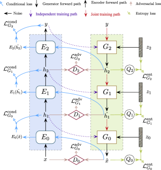
Figure 1: An overview of SGAN depicting a 3-stack model, with the bottom-up encoder stack $E$ in the left box and the top-to-bottom generator stack $G$ to the right. In this case we see stack $G$ being trained jointly. The ordering of the stacks refers to the direction of their respective input. Image taken from [9] and adjusted to fit a smaller frame.

(a) Noiseless Joint PPGN-$h$. Here the encoder $E$ outputs a code $h$ which is the input to the generator $G$. We also see a classifier $C$, used in the MALA-approx sampler, that takes generated images $\hat{x}$ and outputs labels.

(b) Proposed network design. An additional discriminator $D_{i}$ is attached to the $i$th layer of encoder $E$. Dashed arrow indicate that both fake and real samples propagate in the direction.

Figure 2: Displaying the schematic of vanilla PPGN in 2a and in 2b our design is shown. We hypothesize that it is possible to train the generator $G$ while having attached discriminator $D_{i}$ to layer $i$ of encoder $E$.

Concurrent to PPGN [15] is SGAN [9], which extends the GAN framework [7] by creating a stack $G$ of $N$ generators $G_{i}$ in a top-to-bottom fashion. The idea is for $G$ to invert a pre-trained stack $E$ of $N$ bottom-up encoders $E_{i}$. The ordering of the stacks, top-to-bottom or bottom-up, reflect the direction of their respective input, see Fig. 1. Every generator $G_{i}$ is fed with a latent code $h_{i+1}$ coming from an encoder $E_{i}$ in stack $E$, injected with a noise vector $z_{i}$ and produces feature $\hat{h}_{i}=G_{i}(h_{i+1},z_{i})$. The generated $\hat{h}_{i}$ is matched with the input to encoder $E_{i}$. Note that this imposes a constriction for creating the stacks, the input/output pairs of the encoder $E_{i}$ must be correctly aligned with the generator $G_{i}$. Training the generative networks is first done independently and then jointly by stacking them. Therefore, $\hat{h}_{i}=G_{i}(\hat{h}_{i+1},z_{i})$ when jointly trained and $\hat{h}_{i}=G_{i}(h_{i+1},z_{i})$ otherwise. The loss for each generator is $\mathcal{L}_{G_{i}}=\mathcal{L}^{\text{adv}}_{G_{i}}+\mathcal{L}^{\text{cond}}_{G_{i}}+\mathcal{L}^{\text{ent}}_{G_{i}}$. The adversarial loss $\mathcal{L}_{G_{i}}^{\text{adv}}=-\log{D_{i}(G_{i}(h_{i+1},z_{i}))}$ is the same as in [7] but modified for hidden representations. $\mathcal{L}^{\text{cond}}_{G_{i}}=f[E_{i}(G_{i}(h_{i+1},z_{i})),h_{i+1}]$ is a conditional loss with some metric $f$ (such as the $L_{2}$ norm for latent codes and cross entropy for object categories) introduced to assure $G_{i}$ uses the conditional input $h_{i+1}$. Lastly $\mathcal{L}^{\text{ent}}_{G_{i}}=-\log(Q_{i}(z_{i}|\hat{h}_{i}))$, where $Q_{i}$ is an auxiliary distribution for the true posterior $P_{i}(z_{i},\hat{h}_{i})$ and practically implemented as a feedforward network. Since minimizing $\mathcal{L}^{\text{ent}}_{G_{i}}$ is tantamount to maximizing a variational lower bound for the conditional entropy $H(\hat{h}_{i}|h_{i+1})$, $\mathcal{L}^{\text{ent}}_{G_{i}}$ assures diversity of $\hat{h}_{i}$ by making the input $z_{i}$ relevant for $G_{i}$ when constructing $\hat{h}_{i}$ [9]. In addition to the ordinary discriminator inherent to the GAN framework, with every pair $(E_{i},G_{i})$ of encoder and generator, a new discriminator $D_{i}$ is introduced that is trained adversarially to tell the hidden representations $(h_{i},\hat{h}_{i})$ apart. The discriminators are trained to minimize the loss $\mathcal{L}_{D_{i}}=-\log(D_{i}(h_{i}))-\log(1-D_{i}(G_{i}(h_{i+1},z_{i})))$ which is similar as in [7] but altered for taking hidden representations as input. Samples are produced by conditioning the top generator in stack $G$ with label $y$ and injecting its noise vector. The output is then fed to the next generator in the stack along with the next noise vector. This process is repeated until $G_{0}$ is reached, which outputs a sample $\hat{x}=\hat{h}_{0}$. SGANs produce high-quality samples for the MNIST [13] and CIFAR-10 [12] datasets.

SGANs introduce the idea to discriminate between hidden representations $(h_{i},\hat{h}_{i})$. In this master’s thesis we will use this approach for the Noiseless Joint PPGN-$h$ model, but instead discriminate between pairs of codes produced entirely by the encoder. As we will see in the following section, this will not impose the constraint abided by SGANs of aligning each generator layer with its corresponding encoder layer.

3 Method

We start with the noiseless variant of the Joint PPGN-$h$ and change its architecture such that it includes new discriminators. Higher layers in the pre-trained encoder $E$ contain abstract features with a space that is smaller in dimension compared to the lower layers. We hypothesize that it possible to train the generator $G$ in PPGN-$h$ with gradients flowing through discriminators that are attached in these compressed, abstract spaces. For layer $i$ in encoder $E$ we attach a discriminator $D_{i}$ to discern fake codes $\hat{h^{i}}=E^{i}(G(h))$ from real ones $h^{i}$ in the associated latent space. We augment the adversarial loss for $G$

$$\textstyle L_{\text{gan}}=-\lambda_{0}\log{D(\hat{x})}-\sum_{j}\lambda_{j}\log{D_{j}(\hat{h}^{j})}$$ (9)

where $\lambda_{j}$ are scaling factors and $D$ is the ordinary discriminator in PPGN-$h$. If we set $\lambda_{0}=1$ and $\lambda_{j}=0$ for $j>0$, then we get back the usual adversarial loss for the generator in PPGN-$h$. Since there is no restriction in [15] for choosing which layers of $E$ to measure $L_{2}$ perceptual losses from, we can adopt the following simple policy. For every discriminator $D_{j}$ we attach, we also include the autoencoder reconstruction loss of each respective layer

$$\textstyle L_{h}=\sum_{j}\alpha_{j}||\hat{h}^{j}-h^{j}||_{2}^{2}$$ (10)

where we have scaling numbers $\alpha_{j}$. The discriminator attached to the latent space of $E^{i}$ use the loss

$$L_{D_{i}}=-\log D_{i}(h^{i})-\log{(1-D_{i}(\hat{h}^{i}))}$$ (11)

which is similar to Eq. 4.

Observe the difference between the discriminators defined in this master’s thesis and in the SGAN paper. Here we tell autoencoder reconstructions $\hat{h}^{i}=E^{i}(G(h))$ apart from codes $h^{i}=E^{i}(x)$. In SGAN hidden fake outputs from $G_{i}$ is directly compared with real inputs to the corresponding encoder network $E_{i}$, i.e. $\hat{h}_{i}=G_{i}(h_{i+1},z_{i})$ against $h_{i}=E_{i-1}(x)$, see Fig. 1 and Fig. 2b. Since fake hidden codes $\hat{h}^{i}$ are produced entirely by encoder $E^{i}$ using fake inputs $\hat{x}$, we do not need to align input/output pairs of encoder and generator layers. Thus, we skip the alignment constraint of SGANs.

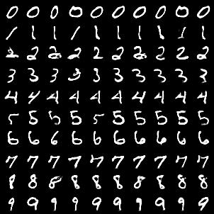
(a) Vanilla PPGN-$h$.

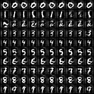
(b) PPGN-$h$-$D_{\textsf{fc1}}$ using $L_{\text{gan}}$.

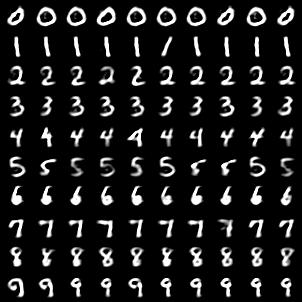
(c) PPGN-$h$-$D_{\textsf{fc1}}$ with full loss.

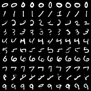
(d) PPGN-$h$-$D_{\textsf{fc1}}$ using $L_{h}$ and $L_{x}$.

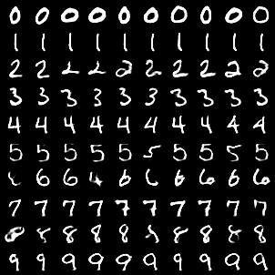
(e) PPGN-$h$-combined.

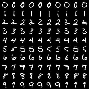
(f) PPGN-$h$-random.

Figure 3: In each figure the samples are produced by the same generator $G$ with fix architecture but trained differently. The parameters of MALA-approx, number of epochs and the scaling factors of each partial loss are the same across every experiment. 3a: We begin with the baseline model Vanilla PPGN-$h$ following the methodology in [15]. We can see some diversity within each class and the generated digits are similar to the MNIST dataset that can be seen in Fig. 5a. We note that class $7$ shows least diversity. 3b: We replace the discriminator $D$ in Vanilla PPGN-$h$ with $D_{\textsf{fc1}}$ to create the PPGN-$h$-$D_{\textsf{fc1}}$ model. For this specific experiment we train $G$ using only the adversarial loss $L_{\text{gan}}$  to see if $G$ is able to converge using only gradients that flow through $D_{\textsf{fc1}}$. The results degrade compared to baseline. Nevertheless, $G$ has learned shapes of every digit class and we can hint some diversity for numbers $0$ and $1$. Evidently, this experiment shows that only including the adversarial loss $L_{\text{gan}}$ with $D_{\textsf{fc1}}$ is not sufficient for generating high-quality samples. 3c: We train PPGN-$h$-$D_{\textsf{fc1}}$ with full loss, i.e. in addition $L_{\text{gan}}$  we also include image loss $L_{x}$  and perceptual similarity loss $L_{h}$. Sampling quality improves but is not quite on a par with baseline. In particular, we notice that the samples do not look as sharp as those generated by Vanilla PPGN-$h$. 3d: Including losses $L_{x}$and $L_{h}$  may have rendered the adversarial loss useless. Given this possibility, we train PPGN-$h$-$D_{\textsf{fc1}}$ but exclude $L_{\text{gan}}$. The samples are of mixed quality, where some digits, such as $0,1,9$, look good relative to baseline while for example $2,4,8$ seem worse. This suggests that the adversarial loss has had an impact on the results in 3c since the samples look different from those produced in this experiment. However, the results for this model are sharper than the samples in 3c. 3e: A new model PPGN-$h$-combined is created by adding the discriminator $D_{\textsf{fc1}}$ to Vanilla PPGN-$h$. We are interested to know whether the model is able to converge when having two different discriminative objective functions for $G$ to minimize. Generated samples are of good quality and is comparable to baseline model. Nonetheless, the training time of this model was considerably longer. 3f: The PPGN-$h$-combined approach showed good results but had longer training time than Vanilla PPGN-$h$. To battle this, we randomized with equal probability which discriminator objective and corresponding adversarial loss to optimize. We refer to this model as PPGN-$h$-random. The approach lead to a reduction in training time while maintaining the higher-quality sampling capability of PPGN-$h$-combined.

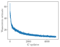
(a) Vanilla PPGN-$h$.

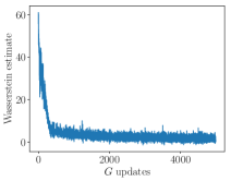
(b) PPGN-$h$-$D_{\textsf{fc1}}$ with full loss.

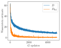
(c) PPGN-$h$-combined.

Figure 4: We chose three models and plot the Wasserstein estimate during training. Every model was able to minimize the metric. The Wasserstein estimate provided by $D_{\textsf{fc1}}$ in Fig. 4b seem easier for $G$ to minimize since it flattens quickly near zero compared to Fig. 4a. A reason might be that $D_{\textsf{fc1}}$ has less capacity relative to $G$. When including both discriminators $D$ and $D_{\textsf{fc1}}$, we can see in Fig. 4c that both Wasserstein estimates are minimized by $G$.

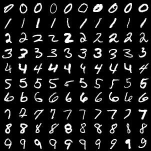
(a) MNIST dataset.

(b) Baseline PPGN-$h$.

(c) PPGN-$h$-random.

Figure 5: To facilitate a comparison between the MNIST dataset, the baseline model and PPGN-$h$-random we showcase them all here. Both of these two models produce samples that resemble MNIST digits, however they do not show as much diversity.

4 Experiments

We use freely available code of a WGAN-GP architecture [19] as a base for implementing the Noiseless Joint PPGN-$h$ model. The WGAN-GP algorithm trains $G$ and $D$ asymmetrically, specifically the discriminator is trained $100$ times for the first $25$ training iterations and the same amount every $500$th. Unless otherwise stated, we use the same hyperparameters as in [19]. For a full overview of hyperparameters and for reproducibility proposes, we publicly release the code used for this master’s thesis.

In every experiment we use the MNIST dataset [13], for which the training set contains $60000$ handwritten digits. Each of these images consist of $28\times 28$ pixels and depicts a number between $0$ and $9$, see Fig. 5a. We normalize the data before feeding it to the entire network.

The encoder $E$ is a convolutional network taken from freely distributed code. However, we modified the architecture and ended up with conv1$(1,64,7)$ $\rightarrow$ conv2$(64,128,7)$ $\rightarrow$ pool2 $\rightarrow$ conv3$(128,256,7)$ $\rightarrow$ pool3 $\rightarrow$ fc1$(256,64)$ $\rightarrow$ fc2$(64,10)$. Notice that the last two layers of $E$, the fully connected layers fc1 and fc2, output vectors of size $64$ and $10$ respectively. Every convolutional and fully connected layer of $E$ is followed by the ReLU activation function, except for fc2. We get the classifier $C$ by applying softmax to fc2. $E$ is pre-trained for classification on MNIST using cross entropy loss and its parameters are held fixed throughout every experiment. The generator $G$ is a deconvolutional network [5] gen-fc1$(64,1600)$ $\rightarrow$ deconv2$(64,512,5)$ $\rightarrow$ deconv3$(512,256,5)$ $\rightarrow$ deconv4$(256,256,7)$ $\rightarrow$ deconv5$(256,1,10)$ and its architecture is held fix. The deconvolutional and fully connected layers of $G$ make use of the ReLU function, with the exception of deconv5 which uses no activation function. All adversarial networks, including discriminators to be defined, are trained using the ADAM optimizer [11], while the encoder $E$ uses the SGD optimizer.

4.1 Vanilla PPGN-$h$

We train PPGN-$h$ using the same losses in [15], where $(\beta_{1},\beta_{2},\beta_{3})$ were set to $(1,10^{-1},2)$ such that every partial loss has the same order of magnitude when training commences. For this experiment we stopped after $15$ epochs of training (roughly $5000$ $G$ updates) using minibatches of size $32$. For the MALA-approx sampler we use parameters $(\epsilon_{1},\epsilon_{2},\epsilon_{3})=(10^{-2},1,10^{-15})$ for $200$ iterations. These values were based on [15], but we have increased the $\epsilon_{1}$ factor to get more generic codes, which yielded better samples. In addition, we increased $\epsilon_{3}$ for more diversity. The number of epochs, size of minibatch, parameters of MALA-approx sampler and the values of $\beta_{k}$ are fixed for every subsequent experiment. $D$ is a CNN with the following architecture, conv1$(1,256,3)$ $\rightarrow$ conv2$(256,256,3)$ $\rightarrow$ pool2 $\rightarrow$ conv3$(256,256,3)$ $\rightarrow$ pool3 $\rightarrow$ conv4$(256,512,3)$ $\rightarrow$ pool4 $\rightarrow$ disc-fc1$(512,1)$ and takes MNIST images $x$ as input. ReLU is used for all layers except the last fully connected layer, which uses no activation function. We take $h$ to be the output of fc1 and we feed it to $G$. Results can be found in Fig. 3a. We plot the estimate of the Wasserstein metric Eq. 2 against generator iterations in Fig. 4a.

4.2 Gradients flowing from fc1 space

We dispense with the ordinary discriminator $D$ in PPGN-$h$ and replace it with $D_{\textsf{fc1}}$ attached to fc1 of $E$. In Eq. 9 this translates to $\lambda_{\text{fc1}}=1$ while all other $\lambda_{j}$ are set to zero. Note that this means that the input of $G$ and $D_{\textsf{fc1}}$ coincide. The autoencoder reconstruction loss Eq. 10 remains unchanged compared to the previous experiment, i.e. $\alpha_{\textsf{fc1}}=1$ and the rest are $\alpha_{j}=0$. $D_{\textsf{fc1}}$ is a CNN with fewer parameters compared to $D$, conv1$(1,256,2)$ $\rightarrow$ conv2$(256,256,2)$ $\rightarrow$ pool2 $\rightarrow$ conv3$(256,512,2)$ $\rightarrow$ pool3 $\rightarrow$ disc-fc1$(512,1)$. The use of activation functions is the same as it was for $D$. We refer to this model as PPGN-$h$-$D_{\textsf{fc1}}$ and train it three times, each with a different loss for $G$. First with only $L_{\text{gan}}$ to exclude the effects of $L_{x}$ and $L_{h}$ in order to investigate if $G$ converges using only gradients that flow through $D_{\textsf{fc1}}$, see Fig. 3b. Thereafter, we train the model with full loss $L_{G}$. Samples for this experiment are found in Fig. 3c and the plot of Wasserstein estimate is in Fig. 4b. Lastly, we use only $L_{x}$ and $L_{h}$ to check if including $L_{\text{gan}}$ has an impact when training PPGN-$h$-$D_{\textsf{fc1}}$ with full loss, results in Fig. 3d.

4.3 Combined approach

We conduct two experiments that include both $D$ and $D_{\textsf{fc1}}$, since we are interested in seeing if the model converges using the two discriminators. In the first experiment, we jointly train $G$ together with $D$ and $D_{\textsf{fc1}}$ using full loss $L_{G}$. Fig. 3e contains the results and in Fig. 4c we find a plot of the Wasserstein estimate Eq. 2. For short, we name this model PPGN-$h$-combined. In the second experiment, we randomly select with equal probability only one pair of adversarial loss to update the network with, i.e. either $D$ and its corresponding adversarial loss for $G$ or $D_{\textsf{fc1}}$ and its adversarial loss. Fig. 3f shows samples from the experiment. This last model is called PPGN-$h$-random.

5 Discussion

The evaluation of generative models is hard [20] and in this section we will visually compare the results in Sec. 4. We realize that this procedure is subjective, but we feel that it is appropriate given the simplicity of the dataset and limited scope of the conclusion we are about to draw. We loosely say that a dataset is simple if it is not diverse enough and point to the fact that MNIST images in each class look somewhat similar. The results could have been quantified using the Inception score method [19], but due to computational costs of using the MALA-approx and the ease of comparing MNIST samples visually we omitted this step. In addition, recent work [3] has shown that using the score for evaluating generative models is problematic.

Images produced by PPGN-$h$-$D_{\textsf{fc1}}$ Fig. 3b used only $L_{\text{gan}}$ loss to take out the effect of training $G$ with losses $L_{x}$ and $L_{h}$. Here we can see that $G$ is able to learn shapes for all digits. Clearly, the samples in Fig. 3b do not resemble MNIST digits to an adequate degree. Therefore, we conclude that it is not sufficient to discriminate between codes $(h,\hat{h})$ using the networks and hyperparameters we have. However, seeing as the generator in this case was able to learn shapes of digits, this prompted us to investigate further. Subsequently, we trained the same model with full loss $L_{G}$ which resulted in improved sampling quality, Fig. 3c. In Fig. 4b we see that the Wasserstein estimate is minimized and flattens quickly. We hypothesize that this is due to capacity discrepancy between $D_{\textsf{fc1}}$ and $G$. Alternatively, fc1-space of $E$ is less complex to minimize the metric over, compared to $X$ space. Furthermore, we cannot be entirely sure that the losses $L_{x}$ and $L_{h}$ made $L_{\text{gan}}$ impractical by interactions unknown to us, but it seems likely that $G$ benefited when $D_{\textsf{fc1}}$ was included given the results in Fig. 3b. Therefore, we trained the same model with only $L_{x}$ and $L_{h}$ to see the effects of excluding the adversarial loss for $G$. The results are shown in Fig. 3d and are somewhat inferior to the samples in Fig. 3c. We note that these models train faster than Vanilla PPGN-$h$ because $D_{\textsf{fc1}}$ has fewer parameters than $D$. Nevertheless, it can be argued that Vanilla PPGN-$h$ could be trained with a slimmer discriminator than the one we had designed while the model at the same time retains same or better sampling quality. We did not experiment extensively with the design of $D$ and the point raised here should not be dismissed lightly.

Our next set of experiments included both $D$ and $D_{\textsf{fc1}}$, where we investigate if the generator $G$ is able converge when including two different discriminators. Judging by the samples in Fig. 3e, we say that this is the case. Furthermore, the model was able to minimize the two different Wasserstein estimates given by the discriminator respectively, as can be seen in Fig. 4c. However, this model is the most complex in the sense that it has the highest number of learnable parameters and took longest to train. Therefore, we trained the same model but randomized which discriminator (and its corresponding adversarial loss for $G$) to update – intention here being to combine the faster training time of PPGN-$h$-$D_{\textsf{fc1}}$ and the better sample quality of Vanilla PPGN-$h$ Fig. 3a. The results in Fig. 3f are comparable to Vanilla PPGN-$h$.

We refrain from taking any further conclusion to the hypothesis, that it is beneficial for $G$ to include discriminators attached to the encoder $E$, other what has been said. This is due to the simplicity of the MNIST dataset. To provide more evidence for the hypothesis we suggest using the method proposed here on more complex datasets and to experiment with more than two discriminators. We raise the issue and leave this for future work.

6 Conclusion

In this master’s thesis we proposed a method of training the Noiseless Joint PPGN-$h$ model by attaching discriminators to different layers of the encoder $E$. We showed that this approach is viable for the MNIST dataset through a series of experiments. Yet, we do not claim that this method generalizes well for other datasets. The reason is that MNIST is a rather simple image manifold, compared to ImageNet and CIFAR-10, and therefore we cannot be certain that the method works well for more complex manifolds.

References

- [1] M. Arjovsky and L. Bottou. Towards principled methods for training generative adversarial networks. arXiv preprint arXiv:1701.04862, 2017.
- [2] M. Arjovsky, S. Chintala, and L. Bottou. Wasserstein gan. arXiv preprint arXiv:1701.07875, 2017.
- [3] S. Barratt and R. Sharma. A note on the inception score. arXiv preprint arXiv:1801.01973, 2018.
- [4] A. Dosovitskiy and T. Brox. Generating images with perceptual similarity metrics based on deep networks. arXiv preprint arXiv:1602.02644, 2016.
- [5] A. Dosovitskiy, J. T. Springenberg, and T. Brox. Learning to generate chairs with convolutional neural networks.
- [6] D. Erhan, Y. Bengio, A. Courville, and P. Vincent. Visualizing higher-layer features of a deep network. University of Montreal, 1341:3, 2009.
- [7] I. J. Goodfellow, J. Pouget-Abadie, M. Mirza, B. Xu, D. Warde-Farley, S. Ozair, A. Courville, and Y. Bengio. Generative adversarial networks. arXiv preprint arXiv:1406.2661, 2014.
- [8] I. Gulrajani, F. Ahmed, M. Arjovsky, V. Dumoulin, and A. Courville. Improved training of wasserstein gans. arXiv preprint arXiv:1704.00028, 2017.
- [9] X. Huang, Y. Li, O. Poursaeed, J. Hopcroft, and S. Belongie. Stacked generative adversarial networks. arXiv preprint arXiv:1612.04357, 2016.
- [10] P. Isola, J.-Y. Zhu, T. Zhou, and A. A. Efros. Image-to-image translation with conditional adversarial networks. arXiv preprint arXiv:1611.07004, 2016.
- [11] D. Kingma and J. Ba. Adam: A method for stochastic optimization. arXiv preprint arXiv:1412.6980, 2014.
- [12] A. Krizhevsky. Learning multiple layers of features from tiny images. 2009.
- [13] Y. LeCun, L. Bottou, Y. Bengio, and P. Haffner. Gradient-based learning applied to document recognition. Proceedings of the IEEE, 86(11):2278–2324, 1998.
- [14] A. Nguyen, A. Dosovitskiy, J. Yosinski, T. Brox, and J. Clune. Synthesizing the preferred inputs for neurons in neural networks via deep generator networks. arXiv preprint arXiv:1605.09304, 2016.
- [15] A. Nguyen, J. Yosinski, Y. Bengio, A. Dosovitskiy, and J. Clune. Plug & play generative networks: Conditional iterative generation of images in latent space. arXiv preprint arXiv:1612.00005, 2016.
- [16] S. Reed, Z. Akata, X. Yan, L. Logeswaran, B. Schiele, and H. Lee. Generative adversarial text to image synthesis. arXiv preprint arXiv:1605.05396, 2016.
- [17] G. O. Roberts and R. L. Tweedie. Exponential convergence of langevin distributions and their discrete approximations. Bernoulli, pages 341–363, 1996.
- [18] O. Russakovsky, J. Deng, H. Su, J. Krause, S. Satheesh, S. Ma, Z. Huang, A. Karpathy, A. Khosla, M. Bernstein, et al. Imagenet large scale visual recognition challenge. arXiv preprint arXiv:1409.0575, 2014.
- [19] T. Salimans, I. Goodfellow, W. Zaremba, V. Cheung, A. Radford, and X. Chen. Improved techniques for training gans. arXiv preprint arXiv:1606.03498, 2016.
- [20] L. Theis, A. v. d. Oord, and M. Bethge. A note on the evaluation of generative models. arXiv preprint arXiv:1511.01844, 2015.
- [21] Y. Wang and M. Kosinski. Deep neural networks are more accurate than humans at detecting sexual orientation from facial images. 2017.