Learning Intrinsic Image Decomposition from Watching the World

Abstract

Single-view intrinsic image decomposition is a highly ill-posed problem, and so a promising approach is to learn from large amounts of data. However, it is difficult to collect ground truth training data at scale for intrinsic images. In this paper, we explore a different approach to learning intrinsic images: observing image sequences over time depicting the same scene under changing illumination, and learning single-view decompositions that are consistent with these changes. This approach allows us to learn without ground truth decompositions, and to instead exploit information available from multiple images when training. Our trained model can then be applied at test time to single views. We describe a new learning framework based on this idea, including new loss functions that can be efficiently evaluated over entire sequences. While prior learning-based methods achieve good performance on specific benchmarks, we show that our approach generalizes well to several diverse datasets, including MIT intrinsic images, Intrinsic Images in the Wild and Shading Annotations in the Wild.

1 Introduction

Intrinsic image decomposition is the problem of factorizing an input image $I$ into a product of a reflectance image and a shading image: $I=R\cdot S$. While the vision community has seen significant advances in single-image intrinsic image decomposition, it remains a challenging, highly ill-posed problem. Hence, the use of machine learning for this task is an appealing prospect. Unfortunately, it is also difficult to gather direct ground truth training data. Previous work has collected ground truth via painting objects [12], synthetic renderings [7, 9], and manual annotation [5, 23], but each of these methods has significant limitations.

Training: we learn from unlabeled indoor and outdoor videos.

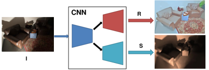Testing: our CNN produces intrinsic images from a single photo.

Figure 1: To train, our method learns from unlabeled videos with fixed viewpoint but varying illumination (top). At test time (bottom), our network produces an intrinsic image decomposition $(R,S)$ from a single image $I$.

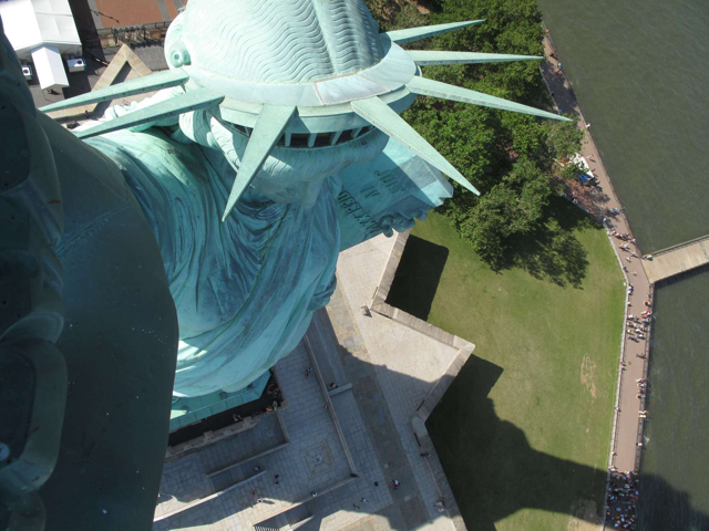
Inspired by how humans can learn by simply observing the world and formulating consistent explanations, we consider an alternative, readily available source of training data for learning intrinsic images: image sequences from the Internet for which the viewpoint is fixed but illumination varies. Based on this idea, we introduce BigTime (BT), a large dataset of time-lapse image sequences. While the sequences in BT do not provide ground truth, they allow us to incorporate useful constraints during training, by specifying that the model should predict outputs consistent with the sequence. While we train on image sequences, our model can apply to a single image at inference time, as illustrated in Figure 1.

Although a number of prior methods estimate intrinsic images from sequences, our concept is quite different: we train on sequences, but learn to infer decompositions from single views. In a sense, our method lies between optimization-based intrinsic images methods and machine learning approaches. In particular, our training loss incorporates priors similar to those of optimization-based approaches, but in a feed-forward prediction framework.

To fully utilize the information present in image sequences, we also introduce two new methods for computing losses over whole sequences, and show how to efficiently implement these losses inside a deep network. The first is an all-pairs weighted least squares loss that considers all pairs of images. The second is a dense, spatio-temporal smoothness loss that jointly considers all of the pixels in the entire sequence. While we use these losses for training intrinsic images, they could also be applied to other problems that involve image sequences, such as video segmentation.

In our evaluation, our method yields competitive or superior performance on two standard real-world benchmarks, IIW and SAW, even when trained on BT without access to annotations from those datasets. We further show improved results on the MIT intrinsic images dataset, even compared to learning methods that utilize full supervised ground truth.

2 Related work

Intrinsic images through optimization. Intrinsic images has been studied for nearly fifty years, often within an optimization framework. Because the problem is ill-posed, additional priors must be applied. For instance, the seminal Retinex algorithm [26] assumes large image gradients correspond to changes in reflectance, while smaller gradients are due to shading. Subsequently, many different priors have been proposed to guide the decomposition [32, 39, 31, 33, 11], and many new optimization tools, such as inference in dense CRFs, have been deployed [5]. Some recent approaches make use of surface normals from RGB-D cameras [10, 3, 19]. Surface normals can improve shading estimates, but such methods assume depth maps are available during optimization.

Intrinsic images from multiple observations. A number of methods, starting with Weiss [37], estimate intrinsic images from time-lapse sequences by assuming constant reflectance but varying shading over time [27, 36, 13, 25, 24]. Such an approach is similar to our training regime, although a crucial distinction is that once our model is trained, we can run it on a single image. These methods rely on priors derived from statistics of image sequences or lighting sources. We found that in practice these methods require $a)$ a large number of input images and $b)$ images taken in outdoor or controlled laboratory environments. In contrast, our method can learn from much shorter and less controlled sequences.

Intrinsic images via supervised learning. Barron and Malik [4] proposed a unified learning-based method that incorporates a number of complex priors on shape, albedo, and illumination. However, their method only applies to single objects and does not generalize well to real-world scenes. Recently, several approaches use deep learning to predict albedo and shading via direct supervision. These methods train on the synthetic Sintel [20, 8], object-centric MIT [12] or synthetic ShapeNet datasets [9, 18]. However, Sintel and ShapeNet are highly synthetic datasets, and networks trained on them do not generalize well to real-world scenes. The MIT dataset consists of real images, but these images depict objects captured in the lab, not realistic scenes, and the dataset contains just 20 objects with ground truth.

Recently, two datasets have been created for real-world scenes. Intrinsic Images in the Wild (IIW) [5] is a dataset of sparse, human-labeled relative reflectance judgments. Shading Annotations in the Wild (SAW) [23] similarly contains sparse shading annotations.Several methods [40, 41, 29, 23] train CNNs on sparse annotations from IIW/SAW and use the predictions as priors for intrinsic images. However, it is difficult to collect such annotations at scale, especially for shading relationships, which can be challenging to perceive. Further, these datasets are limited to sparse annotations. We propose an alternative form of training data that is much easier to capture and provides full-image constraints.

3 Overview and network architecture

Figure 2: System overview and network. During training, our network input is an image sequence $\mathcal{I}$, and the outputs are reflectance images $\mathcal{R}$ and shading images $\mathcal{S}$ for the sequence. Each block in the network depicts a convolutional/deconvolutional layer. $E$ is an encoder, and $D_{R}$ and $D_{S}$ are decoders for the reflectance and shading images. For the innermost feature maps, we have one side output $c$ representing the illumination color. $\mathcal{E}$ is an energy function measuring the cost of the decomposition.

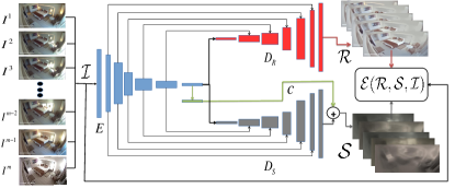
Our work makes two main contributions: a new dataset, BigTime, of image sequences for learning intrinsic images (Sec. 4), and a new approach to learning single-view intrinsic images from this data (Sec. 5). Because we train from image sequences, one learning approach would be to use existing sequence-based intrinsic images algorithms to produce approximate ground truth decompositions, then use these algorithmic outputs as supervision. However, we found that for many image sequences, existing sequence-based algorithms perform poorly because their assumptions are not met, as discussed in Sec. 4. Hence, during training, our CNN directly takes an image sequence as input, and processes it in a feed-forward fashion to produce reflectance and shading for each image in the sequence, as shown in Figure 2. Because the network processes each image independently, at test time multiple images are not required, i.e., we can use the network to produce a decomposition for a single image. During training, the input images interact through our novel loss function (Sec. 5), which evaluates the predicted decompositions jointly for the entire sequence.

For our network, we use a variant of the U-Net architecture [30, 16] (Figure 2). Our network has one encoder and two decoders, one for log-reflectance and one for log-shading, with skip connections for both decoders. Each layer of the encoder consists mainly of a $4\times 4$ stride-2 convolutional layer followed by batch normalization [15] as well as leaky ReLu [14]. For the two decoders, each layer is composed of a $4\times 4$ deconvolutional layer followed by ReLu. In addition to the decoders for reflectance and shading, the network predicts one side output from the innermost feature maps, a single RGB vector for each image corresponding to the predicted illumination color.

4 Dataset

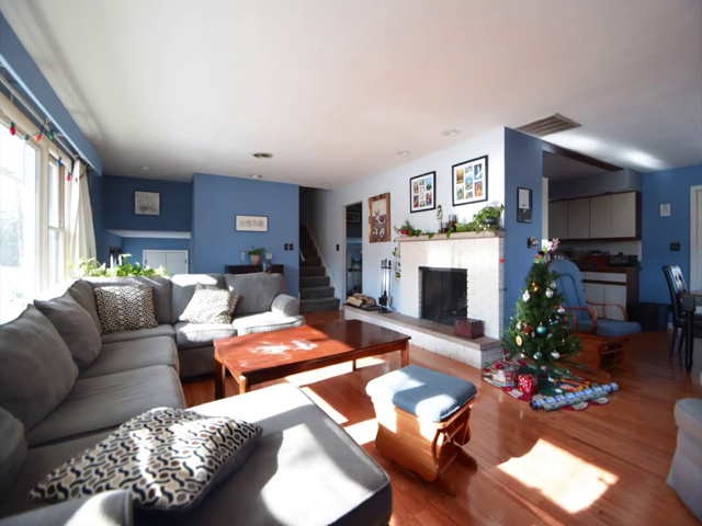
To create the BigTime dataset, we collected videos and image sequences depicting both indoor and outdoor scenes with varying illumination. While many time-lapse datasets primarily capture outdoor scenes, we explicitly wanted representation from indoor scenes as well. Our indoor sequences were gathered from Youtube, Vimeo, Flickr, Shutterstock, and Boyadzhiev et al. [6], and our outdoor sequences were collected from the AMOS [17] and Time Hallucination [35] datasets. For each video, we masked out the sky as well as dynamic objects such as pets, people, and cars via automatic semantic segmentation [38] or manual annotation. We collected 145 sequences from indoor scenes and 50 from outdoor scenes, yielding a total of $\sim$6,500 training images.

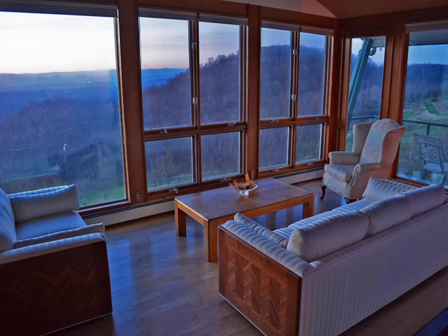
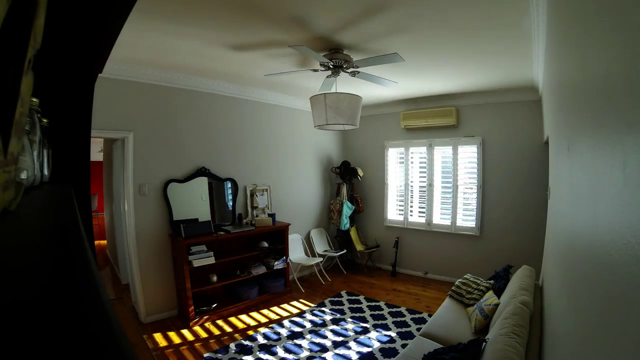
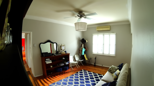
Challenges with Internet videos. Most outdoor scenes in our dataset are from time-lapse sequences where the sun moves evenly over time. Many existing algorithms for multi-image intrinsic image decomposition work well on such data. However, we found that indoor image sequences are much more challenging because illumination changes in indoor scenes tend to be less even or continuous compared to outdoor scenes. In particular, we observed that:

1. most relevant video clips cover a short period of time and do not show large changes in light direction,

2. several video clips are comprised of a light turning on/off in a room, producing a limited number ($<$8) of valid images with different lighting conditions, and

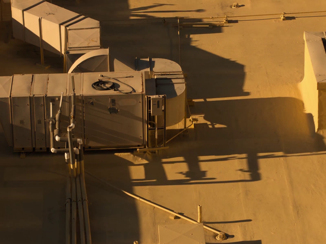
3. the dynamic range of indoor scenes can be high, with strong sunlight or shadows leading to saturation/clipping that can break intrinsic image algorithms.

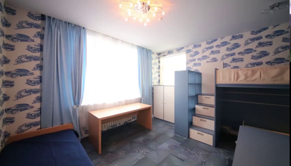
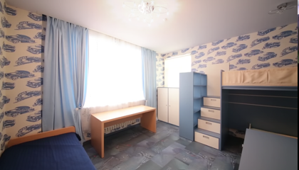
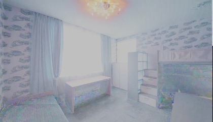
These properties make our dataset even more complex than the IIW and SAW datasets. Several difficult examples are shown in Fig. 3. We found that prior intrinsic image methods designed for image sequences often fail on our indoor videos, as their assumptions tend to hold only for outdoor or lab-captured sequences. Example failure cases are shown in Fig. 4. However, as we show in our evaluation, our approach is robust to such strong illumination conditions, and networks trained on BT generalize well to IIW and SAW.

Figure 3: Examples of challenging images in our dataset. The first two images depict colorful illumination. The last two images show strong sunlight/shadows.

Image	Estimated $R$	Estimated $S$

Figure 4: Failure cases for intrinsic image estimation algorithms. We applied a state-of-the-art multi-image intrinsic image decomposition estimation algorithm [13] to our dataset. This method fails to produce decomposition results suitable for training due to strong assumptions that hold primarily for outdoor/laboratory scenes.

5 Approach

In this section, we describe our novel framework for learning reflectance and shading from Internet time-lapse video clips. During training, we formulate the problem as a continuous densely connected conditional random field (dense CRF) and learn a deep neural network to directly predict a decomposition from single views in a feed-forward fashion.

Image formation model. Let $I$ denote an input image, and $R$ and $S$ denote the predicted reflectance (albedo) and shading. Assuming an image of a Lambertian scene, we can write the image decomposition in the log domain as:

$$\log I=\log R+\log S+N$$ (1)

where $N$ models image noise as well as deviations from a Lambertian assumption. In our model, $S$ is a single-channel (grayscale) image, while $R$ is an RGB image. However, modeling $S$ with a single channel assumes white light. In practice, the illumination color can vary across each input video (for instance, red illumination at sunset/sunrise). Hence, we also allow for a colored light in our model:

$$\log I=\log R+\log S+c+N$$ (2)

where $c$ is a single RGB vector that is added to each element of the left-hand side. For simplicity, we use Eq. 1 in the following sections; without loss of generality, we treat $c$ as being folded into the predicted shading. Each training instance is a stack of $m$ input images with $n$ pixels taken from a fixed viewpoint and varying illumination. We denote such an image sequence by $\mathcal{I}=\left\{I^{i}|i=1\ldots m\right\}$, and denote the corresponding predicted reflectances and shadings by $\mathcal{R}=\left\{R^{i}|i=1\ldots m\right\}$, and $\mathcal{S}=\left\{S^{i}|i=1\ldots m\right\}$, respectively. Additionally, for each image $I^{i}$ we have a binary mask $M^{i}$ indicating which pixels are valid (which we use to exclude saturated pixels, sky, dynamic objects, etc).

We wish to devise a method for learning single-view intrinsic image decomposition that leverages having multiple views during training. Hence, we propose to combine learning and estimation by encoding our priors into the training loss function. Essentially, we learn a feed-forward predictor for single-image intrinsic images, trained on image sequences with a loss that incorporates these priors, and in particular priors that operate at the sequence level. This loss should also be differentiable and efficient to evaluate, considerations which guide our design below.

Energy/loss function.

During training, we formulate the problem as a dense CRF over an image sequence $\mathcal{I}$, where our goal is to maximize a posterior probability $p(\mathcal{R},\mathcal{S}|\mathcal{I})=\frac{1}{Z(\mathcal{I})}\exp\left(-\mathcal{E}(\mathcal{R},\mathcal{S},\mathcal{I})\right)$, where $Z(\mathcal{I})$ is the partition function. Maximizing $p(\mathcal{R},\mathcal{S}|\mathcal{I})$ is equivalent to minimize an energy function $\mathcal{E}(\mathcal{R},\mathcal{S},\mathcal{I})$. Because we use a feed-forward network to predict the decomposition, we also use this energy function as our training loss. We define $\mathcal{E}$ as:

$$\mathcal{E}(\mathcal{R},\mathcal{S},\mathcal{I})= \mathcal{L}_{\mathsf{reconstruct}}+w_{1}\mathcal{L}_{\mathsf{consistency}}+w_{2}\mathcal{L}_{\mathsf{rsmooth}}$$

$$+w_{3}\mathcal{L}_{\mathsf{ssmooth}}$$ (3)

We now describe each term in Eq. 3 in detail.

5.1 Image reconstruction loss

Given an input sequence $\mathcal{I}$, for each image $I^{i}\in\mathcal{I}$ we expect the predicted reflectance and shading for $I^{i}$ to approximately reconstruct $I^{i}$ via our image formation model. Moreover, since reflectance is constant over time, we should be able to use the reflectance $R^{j}$ predicted for any image $I^{j}\in\mathcal{I}$ to reconstruct $I^{i}$, when paired with $S^{i}$ (and masked by the valid image regions indicated by binary masks $M^{i}$ and $M^{j}$). This yields a term involving all pairs of images:

$$\mathcal{L}_{\mathsf{reconstruct}}=\\ \sum_{i=1}^{m}\sum_{j=1}^{m}\left\lVert L^{i}\otimes M^{i}\otimes M^{j}\otimes(\log I^{i}-\log R^{j}-\log S^{i})\right\rVert^{2}_{F}$$ (4)

where $\otimes$ is the Hadamard product. Similar to [10], we weight our reconstruction loss by input pixel luminance $L^{i}=\text{lum}(I^{i})^{\frac{1}{8}}$, since dark pixels tend to be noisy, and image differences in dark regions are magnified in log-space.

We found that including such an all-pairs connected image reconstruction loss improves prediction results, perhaps because it creates more communication between predictions. A direct implementation of this loss takes time $O(m^{2}n)$. In Sec. 5.5 we introduce a computational trick that reduces this to $O(mn)$ time, which is key to making training tractable.

5.2 Reflectance consistency

We also include a reflectance consistency loss that directly encodes the assumption that the predicted reflectances should be identical across the image sequence:

$$\mathcal{L}_{\mathsf{consistency}}=\sum_{i=1}^{m}\sum_{j=1}^{m}\left\lVert M^{i}\otimes M^{j}\otimes(\log R^{i}-\log R^{j})\right\rVert^{2}_{F}$$ (5)

As above, this can be directly computed in time $O(m^{2}n)$, but Sec. 5.5 shows how to reduce this to $O(mn)$.

5.3 Dense spatio-temporal reflectance smoothness

Our reflectance smoothness term $\mathcal{L}_{\mathsf{rsmooth}}$ is based on the similarity of chromaticity and intensity between pixels. Because we see a sequence of images at training time, we can define a reflectance smoothness term that acts jointly on all of the images in each sequence at once, allowing us to express smoothness in a richer way. Accordingly, we introduce a novel spatio-temporal densely connected reflectance smoothness term that considers the similarity of the predicted reflectance at each pixel in the sequence to all other pixels in the sequence. Our method is inspired by the bilateral-space stereo method of Barron et al. [2], but we show how to apply their single-image dense solver to an entire image sequence and how to implement it inside a deep network. We define our smoothness term as:

$$\mathcal{L}_{\mathsf{rsmooth}}=\frac{1}{2}\sum_{I^{i},I^{j}}\sum_{\begin{subarray}{c}p\in I^{i}\\ q\in I^{j}\end{subarray}}\hat{W}_{pq}(\log R^{i}_{p}-\log R^{j}_{q})^{2}\\$$ (6)

where $p$ and $q$ indicate pixels in the image sequence, and $\hat{W}$ is a (bistochastic) weight matrix capturing the affinity between any two pixels $p$ and $q$. Computing this equation directly is very expensive because it involves all pairs of pixels in the sequence, hence we need a more efficient approach.

First, note that if $\hat{W}$ is a bistochastic matrix, we can rewrite Eq. 6 in the following simplified matrix form:

$$\mathcal{L}_{\mathsf{rsmooth}}=\mathbf{r}^{\top}(I-\hat{W})\mathbf{r}$$ (7)

where $\mathbf{r}$ is a stacked vector representation (of length $mn$) of all of the predicted log-reflectance images in the sequence: $\mathbf{r}=[\mathbf{r}^{1}\ \mathbf{r}^{2}\cdots\ \mathbf{r}^{m}]^{\top}$, where $\mathbf{r}^{i}$ is a vector containing the values in $\log R^{i}$. However, now we have a potentially dense affinity matrix $\hat{W}\in\mathbb{R}^{mn\times mn}$. But we can approximately evaluate this term much more efficiently if the pixel-wise affinities are Gaussian, i.e.,

$$W_{pq}=\exp\left(-(\mathbf{f}_{p}-\mathbf{f}_{q})^{\top}\Sigma^{-1}(\mathbf{f}_{p}-\mathbf{f}_{q}))\right)$$ (8)

where $\mathbf{f}_{p}$ and $\mathbf{f}_{q}$ are feature vectors for pixels $p$ and $q$ respectively, and $\Sigma$ is a covariance matrix. We can approximately minimize Eq. 7 in bilateral space by factorizing the Gaussian affinity matrix $W\approx S^{\top}\bar{B}S$, where $\bar{B}=B_{0}B_{1}\cdots B_{d}+B_{d}B_{d-1}\cdots B_{0}$ is a symmetric matrix constructed as a product of sparse matrices representing blur operations in bilateral space, $d$ is the dimension of feature vector $\mathbf{f}_{p}$, and $S$ is a sparse splat/slicing matrix that transforms between image space and bilateral space. Finally, let $\hat{W}=NWN$ be a bistochastic representation of $W$, where $N$ is a diagonal matrix that bistochasticizes $W$ [22]. This bilateral embedding allows us to write the loss in Eq. 7 as:

$$\mathcal{L}_{\mathsf{rsmooth}}\approx\mathbf{r}^{\top}(I-NS^{\top}\bar{B}SN)\mathbf{r}$$ (9)

Note that $\mathcal{L}_{\mathsf{rsmooth}}$ is differentiable and $N$ and $S$ are both sparse matrices that can be computed efficiently. Our final form of $\mathcal{L}_{\mathsf{rsmooth}}$ (Eq. 9) can be computed in time $O((d+1)mn)$, rather than $O(m^{2}n^{2})$.

We define the feature vector used to compute the affinities in Eq. 8 as $\mathbf{f}_{p}=[\ x_{p},y_{p},I_{p},c_{1},c_{2}\ ]^{\top}$, where $(x_{p},y_{p})$ is the spatial position of pixel $p$ in the image, $I_{p}$ is the intensity of $p$, and $c_{1}=\frac{R}{R+G+B}$ and $c_{2}=\frac{G}{R+G+B}$ are the first two elements of the $L_{1}$ chromaticity of $p$.

5.4 Multi-scale shading smoothness

In addition to a reflectance smoothness term, our loss also incorporates a shading smoothness term, $\mathcal{L}_{\mathsf{ssmooth}}$. This term is summed over each predicted shading image: $\mathcal{L}_{\mathsf{ssmooth}}=\sum_{i=1}^{m}L_{\mathsf{ssmooth}}(S^{i})$, where $L_{\mathsf{ssmooth}}(S^{i})$ is defined as a weighted $L_{2}$ term over neighboring pixels:

$$L_{\mathsf{ssmooth}}(S^{i})=\sum_{p\in I^{i}}\sum_{q\in N(p)}v_{pq}\left(\log S^{i}_{p}-\log S^{i}_{q}\right)^{2}$$ (10)

where $N(p)$ denotes the 8-connected neighborhood around pixel $p$, and $v_{pq}$ is a weight on each edge. Our insight is to leverage all of the input images to compute the weights for each individual image. We are inspired by Weiss [37], who derives a multi-image intrinsic images algorithm based on median image derivatives over the sequence. Essentially, we expect the median image derivative over the input sequence (in the log domain) to approximate the derivative of the reflectance image. If we denote $J_{pq}=\log I_{p}-\log I_{q}$ (dropping the image index $i$ for convenience), then this suggests a weight of the form:

$$v^{\mathsf{med}}_{pq}=\exp\left(-\lambda^{\mathsf{med}}\left(J_{pq}-\mathrm{median}\{J_{pq}\}\right)^{2}\right)$$ (11)

where $\mathrm{median}\{J_{pq}\}$ is the median value of $J_{pq}$ over the image sequence, and $\lambda^{\mathsf{med}}$ is a parameter defining the strength of $v^{\mathsf{med}}_{pq}$. This weight discourages shading smoothness where the gradient of a particular image is very different from the median (as would happen, e.g., for a shadow boundary).

Image	$v^{\mathsf{med}}_{pq}$	$\max\{v^{\mathsf{med}}_{pq},\overline{v^{\mathsf{med}}_{pq}}\}$	$v_{pq}$

Figure 5: Effect of $\overline{v^{\mathsf{med}}}$ in shading smoothness term. (white $=$ large weight, black $=$ small weight.) Adding the extra $\overline{v^{\mathsf{med}}}$ can help capture smoothness in textured regions such as the pillows in the first row and floor in the second row. The last column shows the final smoothness weight $v_{pq}$.

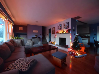
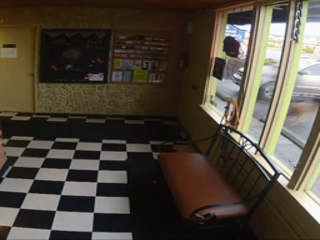
We found that $v^{\mathsf{med}}_{pq}$ works well as a weight for texture-less regions (for instance, it captures the effect of a cast shadow on a flat wall well), but, due to noise present in dark image regions, it does not always capture the desired shading smoothness for textured surfaces. Figure 5 (bottom) illustrates such a case with a checkerboard pattern on the floor. To address this issue, we define an additional weight $\overline{v^{\mathsf{med}}_{pq}}$ that is normalized by the median derivative:

$$\overline{v^{\mathsf{med}}_{pq}}=\exp\left(-\overline{\lambda^{\mathsf{med}}}\left(\frac{J_{pq}-\mathrm{median}\{J_{pq}\}}{\mathrm{median}\{J_{pq}\}}\right)^{2}\right)$$ (12)

We combine these weights as follows:

$$v_{pq}=\max\{v^{\mathsf{med}}_{pq},\overline{v^{\mathsf{med}}_{pq}}\}\cdot\left(1-\mathrm{median}\{W_{pq}\}\right)$$ (13)

This final shading smoothness weight is more robust to textured regions while still distinguishing shadow discontinuities. The last factor $\left(1-\mathrm{median}\{W_{pq}\}\right)$ reflects the belief that we should enforce stronger shading smoothness on reflectance edges such as textures and weaker smoothness on regions of constant reflectance.

Ideally, our shading smoothness term would be densely connected. However, the median operator is nonlinear and cannot be integrated in a pixel-wise densely connected term. Instead, to introduce longer-range shading constraints, we compute the shading smoothness term at multiple image scales, by repeatedly downsizing each predicted shading image by a factor of two. We set the number of scales to be 4, and each scale $l$ is weighted by a factor $\frac{1}{l}$.

5.5 All-pairs weighted least squares (APWLS)

Direct implementations of the all-pairs image reconstruction and reflectance consistency terms from Sections 5.1 and 5.2 would take $O(m^{2}n)$ time. This quadratic complexity would make training intractable for large enough $m$. Here, we propose a closed-form version of this all-pairs weighted least squares loss (APWLS) that is linear in $m$. While we apply this tool to our scenario, it can be used in other situations involving all-pairs computation on image sequences.

In general, suppose each image $I^{i}$ is associated with two matrices $P^{i}$ and $Q^{i}$ and two prediction images $X^{i}$ and $Y^{i}$. We then can write APWLS as (see supplemental material for a detailed derivation):

$$\text{APWLS}= \sum_{i=1}^{m}\sum_{j=1}^{m}||P^{i}\otimes Q^{j}\otimes(X^{i}-Y^{j})||^{2}_{F}$$ (14)

$$= \mathbf{1}^{\top}(\Sigma_{Q^{2}}\otimes\Sigma_{P^{2}X^{2}}+\Sigma_{P^{2}}\otimes\Sigma_{Q^{2}Y^{2}}-$$

$$2\Sigma_{P^{2}Y}\otimes\Sigma_{Q^{2}X})\mathbf{1}$$ (15)

where $\Sigma_{Z}$ denotes the sum over all images of the Hadamard product indicated in the subscript $Z$. Evaluating Eq. 14 requires time $O(m^{2}n)$, but rewritten as Eq. 15, just $O(mn)$.

We use this derivation to implement our image reconstruction loss $\mathcal{L}_{\mathsf{reconstruct}}$ (Eq. 15), by making the substitutions $P^{i}=L^{i}\otimes M^{i}$, $Q^{j}=M^{j}$, $X^{i}=\log I^{i}-\log S^{i}$ and $Y^{j}=\log R^{j}$, and our reflectance consistency loss $\mathcal{L}_{\mathsf{consistency}}$ (Eq. 5) by substituting $P^{i}=M^{i}$, $Q^{j}=M^{j}$, $X^{i}=\log R^{i}$ and $Y^{j}=\log R^{j}$.

6 Evaluation

In this section we evaluate our approach by training solely on our BigTime dataset, and testing on two standard datasets, IIW and SAW. The performance of machine learning approaches can suffer from cross-dataset domain shift due to dataset bias. For example, we show that the performance of networks trained on Sintel, MIT, or ShapeNet do not generalize well to IIW and SAW. However, our method, though not trained on IIW or SAW data, can still produce competitive results on both datasets. We also evaluate on the MIT intrinsic images dataset [12], which has full ground truth. Rather than using the ground truth during training, we train the network on image sequences provided by the MIT dataset.

Training details. We implement our method in PyTorch [1]. In total, we have 195 image sequences for training. We perform data augmentation via random rotations, flips, and crops. When feeding images into the network, we resize them to $256\times 384$, $384\times 256$, or $256\times 256$ depending on the original aspect ratio. For all evaluations, we train the network from scratch using Adam [21].

6.1 Evaluation on IIW

Method	Training set	WHDR%
Retinex-Color [12]	-	26.9
Garces et al. [11]	-	24.8
Zhao et al. [39]	-	23.8
Bell et al. [5]	-	20.6
Narihira et al. [29]∗	IIW	18.1∗
Zhou et al. [40]∗	IIW	15.7∗
Zhou et al. [40]	IIW	19.9
DI [28]	Sintel+MIT	37.3
Shi et al. [34]	ShapeNet	59.4
Ours (w/ per-image $\mathcal{L}_{\mathsf{reconstruct}}$)	BT	25.9
Ours (w/ local $\mathcal{L}_{\mathsf{rsmooth}}$)	BT	27.4
Ours (w/ grayscale $S$)	BT	22.3
Ours (full method)	BT	20.3

Table 1: Results on the IIW test set. Lower is better for the Weighted Human Disagreement Rate (WHDR). The second column indicates the training data each learning-based method uses; “-” indicates the method is optimization-based. ^∗ indicates WHDR is evaluated based on CNN classifer outputs for pairs of pixels rather than full decompositions.

Method	Training set	AP%
Retinex-Color [12]	-	91.93
Garces et al. [11]	-	96.89
Zhao et al. [39]	-	97.11
Bell et al. [5]	-	97.37
Zhou et al. [40]	IIW	96.24
DI [28]	Sintel+MIT	95.04
Shi et al. [34]	ShapeNet	86.30
Ours (w/ local $\mathcal{L}_{\mathsf{ssmooth}}$)	BT	97.03
Ours (w/o Eq. 12)	BT	97.15
Ours (full method)	BT	97.90

Table 2: Results on the SAW test set. Higher is better for AP%. The second column is described in Table 1. Note that none of the methods use annotations from SAW.

(a) Image

(b) Bell et al. (R)

(c) Bell et al. (S)

(d) Zhou et al. (R)

(e) Zhou et al. (S)

(f) Ours (R)

(g) Ours (S)

Figure 6: Qualitative comparisons for intrinsic image decomposition on the IIW/SAW test sets. Our network predictions achieve comparable results to state-of-art intrinsic image decomposition algorithms (Bell et al. [5] and Zhou et al. [40]).

To evaluate on the IIW dataset, we train our network on BT (without using IIW training data) and directly apply our trained model on the IIW test split provided by [29]. Numerical comparisons between our method and other optimization-based and learning-based approaches are shown in Table 1. Our method is competitive with both optimization-based methods [5] and learning-based methods [40]. Note that the best WHDR (marked ^∗) in the table is achieved using CNN classier outputs on pairs of pixels, rather than full image decompositions. In contrast, our results are based on full decompositions. Additionally, as we show in the next subsection, the best performing method (Zhou et al. [40]) on IIW (which primarily evaluates reflectance) falls behind on SAW (which evaluates shading), suggesting that their method tends to overfit on reflectance. shading accuracy. We also see that networks trained on Sintel, MIT or ShapeNet perform poorly on IIW, likely due to dataset bias.

We also perform an ablation study on different configurations of our framework. First, we modify the image reconstruction loss to an alternate loss that considers each image independently, rather than considering all pairs of images in a sequence. Second, we evaluate a modified reflectance smoothness loss that uses local pairwise smoothness (between neighboring pixels) rather than our proposed dense spatio-temporal smoothness. Finally, we try using grayscale shading, rather than our colored shading. The results, shown in the last four rows of Table 1, demonstrate that our full method can significantly improve reflectance predictions on the IIW test set compared to simpler configurations.

6.2 Evaluation on SAW

			MSE				LMSE				DSSIM
Method	Training set	GT	refl.	shading	avg.		refl.	shading	avg.		refl.	shading	avg.
SIRFS [4]	MIT	Yes	0.0147	0.0083	0.0115		0.0416	0.0168	0.0292		0.1238	0.0985	0.1111
DI [28]	MIT+ST	Yes	0.0277	0.0154	0.0215		0.0585	0.0295	0.0440		0.1526	0.1328	0.1427
Shi [34]	MIT+SN	Yes	0.0278	0.0126	0.0202		0.0503	0.0240	0.0372		0.1465	0.1200	0.1332
Ours	MIT	No	0.0147	0.0135	0.0141		0.0341	0.0253	0.0297		0.1398	0.1266	0.1332

Table 3: Results on MIT intrinsics. For all error metrics, lower is better. ST$=$Sintel dataset and SN$=$ShapeNet dataset. The second column shows the dataset used for training. GT indicates whether the method uses ground truth for training.

Next, we test our network on SAW [23], again training without using data from SAW. We also propose two improvements to the metric used to evaluate results on SAW:

First, the original SAW error metric is based on classifying a pixel $p$ as having smooth/nonsmooth shading based on the gradient magnitude of the predicted shading image, $||\nabla S||_{2}$, normalized to the range $[0,1]$. Instead, we measure the gradient magnitude in the log domain. We do this because of the scale ambiguity inherent to shading and reflectance, and because it is possible to have very bright values in the shading channel (e.g., due to strong sunlight), and in such cases if we normalize shading to $[0,1]$ then most of the resulting values will be close to 0. In contrast, computing the gradient magnitude of log shading $||\nabla\log S||_{2}$ achieves scale invariance, resulting in fairer comparisons for all methods. As in [23], we sweep a threshold $\tau$ to create a precision-recall (PR) curve that captures how well each method captures smooth and non-smooth shading.

Second, Kovacs et al.  [23] apply a $10\times 10$ maximum filter to the shading gradient magnitude image before computing PR curves, because many shadow boundary annotations are not precisely localized. However, this maximum filter can result in degraded performance for smooth shading regions. Instead, we use the max-filtered log-gradient-magnitude image when classifying non-smooth annotations, but use the unfiltered log gradient image when classifying smooth annotations (see supplementary for details).

All methods, including our own, are trained without use of SAW data. Average precision (AP) scores are shown in Table 2 (please see the supplementary for full precision-recall curves). Our method has the best performance among all prior methods we tested, and our full loss outperforms variants with terms removed. In particular, our method outperforms the best optimization-based algorithm [5] on both IIW and SAW. On the other hand, Zhou et al. [40] tends to overfit to IIW, as their performance on SAW ranks lower than several other methods. Again, networks trained on Sintel, MIT, and ShapeNet data perform poorly on SAW.

6.3 Qualitative results on IIW and SAW

Figure 6 shows qualitative results from our method and two other state-of-art intrinsic image decomposition algorithms, Zhou et al. [40] and Bell et al. [5], on test images from IIW and SAW. Our results are visually comparable to these methods. One observation is that our shading predictions for dark pixels can be quite dark, leading to reduced contrast in the reflectance images. However, this loss of contrast does not hurt numerical performance. Additionally, like other CNN approaches [28, 34], the direct predictions from our network may not strictly satisfy $I=R\cdot S$ since the two decoders predict $R$ and $S$ simultaneously at test time. As future work, it would be interesting to use our predictions as priors for optimization to address these issues.

6.4 Evaluation on MIT intrinsic images

The MIT intrinsic images dataset [12] contains 20 objects with ground truth reflectance and shading, as well as an associated image sequence taken from 11 different directional light sources. We use the same training-test split as in Barron et al. [4], but instead of training our network on the ground truth provided by the MIT dataset, we train only on the provided image sequences using our learning approach. In this case, we configure our network to produce grayscale shading outputs, since the MIT dataset only contains grayscale shading ground truth images.

We compare our approach to several supervised learning methods including SIRFS [4], Direct Intrinsics (DI) [28] and Shi et al. [34]. These prior methods all train using ground truth reflectance and shading images, and additionally DI [28] and Shi et al. [34] pretrain on Sintel [7] and ShapeNet [9], respectively. In contrast, we train our network from scratch and only use the provided image sequences during training. We adopt the same metrics as [34], including mean square error (MSE), local mean square error (LMSE), and structural dissimilarity index (DSSIM).

(a) Image	(b) GT	(c) SIRFS	(d) DI	(e)Shi et al.	(f)Ours

Figure 7: Qualitative comparisons on the MIT intrinsic test set. Odd-number rows show predicted reflectance; even-numbered rows show predicted shading. (a) Input image, (b) Ground truth (GT), (c) SIRFS [4], (d) Direct Intrinsics (DI) [28], (e) Shi et al. [34], (f) Our method.

Numerical results are shown in Table 3 and qualitative comparisons are shown in Figure 7. Averaged over reflectance and shading, our results numerically outperform both prior CNN-based supervised learning methods [28, 34]. In particular, our albedo estimates are significantly better, while our shading estimates are comparable (slightly better than [28], and slightly worse than [34]). SIRFS has the best numerical results on the MIT, but SIRFS’s priors only apply to single objects, and their algorithm performs much more poorly on full images of real-world scenes [28, 34].

7 Conclusion

We presented a new method for learning intrinsic images, supervised not by ground truth decompositions, but instead by simply observing image sequences with varying illumination over time, and learning to produce decompositions that are consistent with these sequences. Our model can then be run on single images, producing competitive results on several benchmarks. Our results illustrate the power of learning decompositions simply from watching large amounts of video. In the future, we plan to combine our approach with other kinds of annotations (IIW, SAW, etc), to measure how well they perform when used together, and to use our outputs as inputs to optimization-based methods.

Acknowledgments. We thank Jingguang Zhou for his help with data collection. We also thank the anonymous reviewers for their valuable comments. This work was funded by the National Science Foundation through grant IIS-1149393, and by a grant from Schmidt Sciences.

References

- [1] Pytorch. 2016. http://pytorch.org.
- [2] J. T. Barron, A. Adams, Y. Shih, and C. Hernández. Fast bilateral-space stereo for synthetic defocus. In Proc. Computer Vision and Pattern Recognition (CVPR), pages 4466–4474, 2015.
- [3] J. T. Barron and J. Malik. Intrinsic scene properties from a single RGB-D image. In Proc. Computer Vision and Pattern Recognition (CVPR), pages 17–24, 2013.
- [4] J. T. Barron and J. Malik. Shape, illumination, and reflectance from shading. Trans. on Pattern Analysis and Machine Intelligence, 37(8):1670–1687, 2015.
- [5] S. Bell, K. Bala, and N. Snavely. Intrinsic images in the wild. ACM Trans. Graphics, 33(4):159, 2014.
- [6] I. Boyadzhiev, S. Paris, and K. Bala. User-assisted image compositing for photographic lighting. ACM Trans. Graphics, 32:36:1–36:12, 2013.
- [7] D. J. Butler, J. Wulff, G. B. Stanley, and M. J. Black. A naturalistic open source movie for optical flow evaluation. In Proc. European Conf. on Computer Vision (ECCV), 2012.
- [8] D. J. Butler, J. Wulff, G. B. Stanley, and M. J. Black. A naturalistic open source movie for optical flow evaluation. In Proc. European Conf. on Computer Vision (ECCV), pages 611–625, 2012.
- [9] A. X. Chang, T. Funkhouser, L. Guibas, P. Hanrahan, Q. Huang, Z. Li, S. Savarese, M. Savva, S. Song, H. Su, et al. ShapeNet: An information-rich 3d model repository. arXiv preprint arXiv:1512.03012, 2015.
- [10] Q. Chen and V. Koltun. A simple model for intrinsic image decomposition with depth cues. In Proc. Computer Vision and Pattern Recognition (CVPR), pages 241–248, 2013.
- [11] E. Garces, A. Munoz, J. Lopez-Moreno, and D. Gutierrez. Intrinsic images by clustering. In Computer graphics forum, volume 31, pages 1415–1424. Wiley Online Library, 2012.
- [12] R. Grosse, M. K. Johnson, E. H. Adelson, and W. T. Freeman. Ground truth dataset and baseline evaluations for intrinsic image algorithms. In Proc. Int. Conf. on Computer Vision (ICCV), pages 2335–2342, 2009.
- [13] D. Hauagge, S. Wehrwein, K. Bala, and N. Snavely. Photometric ambient occlusion. In Proc. Computer Vision and Pattern Recognition (CVPR), pages 2515–2522, 2013.
- [14] K. He, X. Zhang, S. Ren, and J. Sun. Delving deep into rectifiers: Surpassing human-level performance on imagenet classification. In Proc. Int. Conf. on Computer Vision (ICCV), pages 1026–1034, 2015.
- [15] S. Ioffe and C. Szegedy. Batch normalization: Accelerating deep network training by reducing internal covariate shift. In Proc. Int. Conf. on Machine Learning, pages 448–456, 2015.
- [16] P. Isola, J.-Y. Zhu, T. Zhou, and A. A. Efros. Image-to-image translation with conditional adversarial networks. In Proc. Computer Vision and Pattern Recognition (CVPR), pages 5967–5976, 2017.
- [17] N. Jacobs, N. Roman, and R. Pless. Consistent temporal variations in many outdoor scenes. In Proc. Computer Vision and Pattern Recognition (CVPR), pages 1–6, 2007.
- [18] M. Janner, J. Wu, T. Kulkarni, I. Yildirim, and J. B. Tenenbaum. Self-supervised intrinsic image decomposition. In Neural Information Processing Systems, 2017.
- [19] J. Jeon, S. Cho, X. Tong, and S. Lee. Intrinsic image decomposition using structure-texture separation and surface normals. In Proc. European Conf. on Computer Vision (ECCV), 2014.
- [20] S. Kim, K. Park, K. Sohn, and S. Lin. Unified depth prediction and intrinsic image decomposition from a single image via joint convolutional neural fields. In Proc. European Conf. on Computer Vision (ECCV), pages 143–159. Springer, 2016.
- [21] D. P. Kingma and J. Ba. Adam: A method for stochastic optimization. arXiv preprint arXiv:1412.6980, 2014.
- [22] P. A. Knight, D. Ruiz, and B. Uçar. A symmetry preserving algorithm for matrix scaling. SIAM Journal on Matrix Analysis and Applications, 35(3):931–955, 2014.
- [23] B. Kovacs, S. Bell, N. Snavely, and K. Bala. Shading annotations in the wild. In Proc. Computer Vision and Pattern Recognition (CVPR), pages 850–859, 2017.
- [24] P.-Y. Laffont and J.-C. Bazin. Intrinsic decomposition of image sequences from local temporal variations. In Proc. Int. Conf. on Computer Vision (ICCV), pages 433–441, 2015.
- [25] P.-Y. Laffont, A. Bousseau, S. Paris, F. Durand, and G. Drettakis. Coherent intrinsic images from photo collections. In ACM Trans. Graphics (SIGGRAPH), 2012.
- [26] E. H. Land and J. J. McCann. Lightness and retinex theory. Josa, 61(1):1–11, 1971.
- [27] Y. Matsushita, S. Lin, S. B. Kang, and H.-Y. Shum. Estimating intrinsic images from image sequences with biased illumination. In Proc. European Conf. on Computer Vision (ECCV), pages 274–286, 2004.
- [28] T. Narihira, M. Maire, and S. X. Yu. Direct intrinsics: Learning albedo-shading decomposition by convolutional regression. In Proc. Int. Conf. on Computer Vision (ICCV), pages 2992–2992, 2015.
- [29] T. Narihira, M. Maire, and S. X. Yu. Learning lightness from human judgement on relative reflectance. In Proc. Computer Vision and Pattern Recognition (CVPR), pages 2965–2973, 2015.
- [30] O. Ronneberger, P. Fischer, and T. Brox. U-net: Convolutional networks for biomedical image segmentation. In Int. Conf. on Medical Image Computing and Computer-Assisted Intervention, pages 234–241. Springer, 2015.
- [31] C. Rother, M. Kiefel, L. Zhang, B. Schölkopf, and P. V. Gehler. Recovering intrinsic images with a global sparsity prior on reflectance. In Neural Information Processing Systems, pages 765–773, 2011.
- [32] L. Shen, P. Tan, and S. Lin. Intrinsic image decomposition with non-local texture cues. In Proc. Computer Vision and Pattern Recognition (CVPR), pages 1–7, 2008.
- [33] L. Shen and C. Yeo. Intrinsic images decomposition using a local and global sparse representation of reflectance. In Proc. Computer Vision and Pattern Recognition (CVPR), pages 697–704, 2011.
- [34] J. Shi, Y. Dong, H. Su, and S. X. Yu. Learning non-lambertian object intrinsics across shapenet categories. Proc. Computer Vision and Pattern Recognition (CVPR), 2017.
- [35] Y. Shih, S. Paris, F. Durand, and W. T. Freeman. Data-driven hallucination of different times of day from a single outdoor photo. ACM Transactions on Graphics (TOG), 32(6):200, 2013.
- [36] K. Sunkavalli, W. Matusik, H. Pfister, and S. Rusinkiewicz. Factored time-lapse video. In ACM Transactions on Graphics (TOG), volume 26, page 101. ACM, 2007.
- [37] Y. Weiss. Deriving intrinsic images from image sequences. In Proc. Int. Conf. on Computer Vision (ICCV), volume 2, pages 68–75, 2001.
- [38] H. Zhao, J. Shi, X. Qi, X. Wang, and J. Jia. Pyramid scene parsing network. Proc. Computer Vision and Pattern Recognition (CVPR), 2017.
- [39] Q. Zhao, P. Tan, Q. Dai, L. Shen, E. Wu, and S. Lin. A closed-form solution to retinex with nonlocal texture constraints. Trans. on Pattern Analysis and Machine Intelligence, 34(7):1437–1444, 2012.
- [40] T. Zhou, P. Krahenbuhl, and A. A. Efros. Learning data-driven reflectance priors for intrinsic image decomposition. In Proc. Int. Conf. on Computer Vision (ICCV), pages 3469–3477, 2015.
- [41] D. Zoran, P. Isola, D. Krishnan, and W. T. Freeman. Learning ordinal relationships for mid-level vision. In Proc. Int. Conf. on Computer Vision (ICCV), pages 388–396, 2015.