Imaging through a scattering medium by speckle intensity correlations

Josselin Garnier(1) and Knut Sølna(2) (1)Centre de Mathématiques Appliquées, Ecole Polytechnique, 91128 Palaiseau Cedex, France josselin.garnier@polytechnique.edu (2)Department of Mathematics, University of California Irvine, Irvine CA 92617 ksolna@math.uci.edu
Abstract

In this paper we analyze an imaging technique based on intensity speckle correlations over incident field position proposed in [J. A. Newmann and K. J. Webb, Phys. Rev. Lett. 113, 263903 (2014)]. Its purpose is to reconstruct a field incident on a strongly scattering random medium. The thickness of the complex medium is much larger than the scattering mean free path so that the wave emerging from the random section forms an incoherent speckle pattern. Our analysis clarifies the conditions under which the method can give a good reconstruction and characterizes its performance. The analysis is carried out in the white-noise paraxial regime, which is relevant for the applications in optics that motivated the original paper.

Keywords: Waves in random media, speckle imaging, multiscale analysis.

1 Introduction

Imaging and communication through a randomly scattering medium is challenging because the coherent incident waves are transformed into incoherent wave fluctuations. This degrades wireless communication [1, 10], medical imaging [19], and astronomical imaging [32]. When scattering is weak, different methods have been proposed, which consists in extracting the small coherent wave from the recorded field [3, 4, 5, 6, 29]. These methods fail when scattering becomes strong and the coherent field completely vanishes. However recent developments have shown that it is possible to achieve wave focusing through a strongly scattering medium by control of the incident wavefront [33, 34, 35]. These results have opened the way to new methods for wave imaging through a strongly scattering medium [21, 25, 28].

In [26] an original imaging method is presented that makes it possible to reconstruct fields incident on a randomly scattering medium from intensity-only measurements. From the experimental point of view, the speckle intensity images are taken as a function of incident field position and then used to calculate the speckle intensity correlation over incident position. From the theoretical point of view, the speckle intensity correlation function is then expressed using a moment theorem as the magnitude squared of the incident field autocorrelation function. The modulus of the spatial Fourier transform of the incident field can then be extracted, and the incident field itself can be reconstructed using a phase retrieval algorithm. The key argument is the moment theorem that is based on a zero-mean circular Gaussian assumption for the transmitted field. In [26] the authors claim that heavy clutter is necessary and sufficient for this. One of the main applications is a new method to view binary stars from Earth (using the Earth’s rotation and atmospheric scatter). Other biomedical applications are proposed and extensions of the technique to imaging hidden objects with speckle intensity correlations over object position have been proposed [27].

In this paper we present a detailed analysis of the technique in the white-noise paraxial regime, which is the regime relevant for the applications [30, 31]. We clarify the conditions under which the imaging approach proposed in [26] can be efficient. In particular, we will see that the zero-mean circular Gaussian assumption is not strictly necessary, however, that strongly scattering media may not create the right conditions for the imaging approach to work well. We can distinguish two strongly scattering regimes, the scintillation regime (in which the correlation radius of the medium fluctuations is smaller than the field radius) and the spot-dancing regime (in which the correlation radius of the medium fluctuations is larger than the field radius), and these regimes give completely different results. In the scintillation regime we will explain that the method proposed by [26] can give a correct image, but not in the spot-dancing regime. In particular, the spot-dancing regime may be relevant for Earth-based astronomy [2], which would let little hope that the method can be used there, but it could be efficient in other configurations in the scintillation regime.

The paper is organized as follows. In Section 2 we describe the experiment and introduce the empirical speckle intensity covariance. In Section 3 we present the white-noise paraxial wave equation. We analyze the properties of the statistical speckle intensity covariance in the scintillation regime in Section 4 and in the spot-dancing regime in Section 5. Section 6 summarizes the main findings.

Refer to caption
Figure 1: The experimental imaging set-up. The source transmits a time-harmonic plane wave. The object to be imaged is a mask. For each position of the mask the intensity of the transmitted field can be recorded by the camera.

2 The intensity covariance function
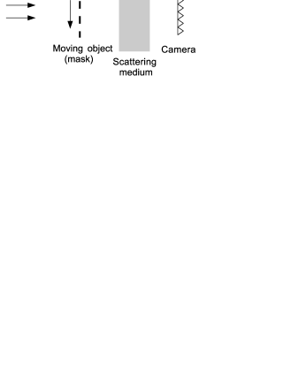
The spatial variable is denoted by $({{\itbf x}},z)\in\mathbb{R}^{d}\times\mathbb{R}$. The source transmits a time-harmonic plane wave going into the $z$-direction with frequency $\omega$ and wavenumber $k_{o}=\omega/c_{o}$, with $c_{o}$ the background velocity. The object to be imaged is a mask (a double slit in the experiment [26]) that can be shifted transversally by a shift vector denoted by ${{\itbf r}}$ so that the field just after the mask is of the form

$$U_{{\itbf r}}({{\itbf x}})=U({{\itbf x}}-{{\itbf r}}),$$ (1)

for some function $U$ (see Figure 1). Note that we here assume that the homogeneous scattering medium fills the space in between the mask and the camera, see also Remark 4.9.

The time-harmonic field in the plane of the camera is denoted by $E_{{\itbf r}}({{\itbf x}})$. It results from the propagation of the incident field $U_{{\itbf r}}$ through the scattering medium. The measured or empirical intensity covariance is

$\displaystyle C_{{{\itbf r}},{{\itbf r}}^{\prime}}$ $\displaystyle=$ $\displaystyle\frac{1}{|A_{o}|}\int_{A_{o}}|E_{{\itbf r}}({{\itbf x}}_{0})|^{2}|E_{{{\itbf r}}^{\prime}}({{\itbf x}}_{0})|^{2}{\rm d}{{\itbf x}}_{0}$ (2)
$\displaystyle-\Big{(}\frac{1}{|A_{o}|}\int_{A_{o}}|E_{{\itbf r}}({{\itbf x}}_{0})|^{2}{\rm d}{{\itbf x}}_{0}\Big{)}\Big{(}\frac{1}{|A_{o}|}\int_{A_{o}}|E_{{{\itbf r}}^{\prime}}({{\itbf x}}_{0})|^{2}{\rm d}{{\itbf x}}_{0}\Big{)},$

where $A_{o}$ is the spatial support of the camera. The conjecture found in [26] is the following one.

Conjecture 2.1
$\displaystyle C_{{{\itbf r}},{{\itbf r}}^{\prime}}\approx\Big{|}\int_{\mathbb{R}^{d}}|\hat{U}({{\itbf k}})|^{2}\exp\big{(}i{{\itbf k}}\cdot({{\itbf r}}^{\prime}-{{\itbf r}})\big{)}{\rm d}{{\itbf k}}\Big{|}^{2},$ (3)

up to a multiplicative constant, where

$$\hat{U}({{\itbf k}})=\int_{\mathbb{R}^{d}}U({{\itbf x}})\exp\big{(}-i{{\itbf k}}\cdot{{\itbf x}}\big{)}{\rm d}{{\itbf x}}.$$ (4)

When this formula holds, it is possible to reconstruct the incident field $U$ by a phase retrieval algorithm as shown in [26]. Indeed (3) gives the modulus of the inverse Fourier transform of $|\hat{U}({{\itbf k}})|^{2}$, and we know the phase of $|\hat{U}({{\itbf k}})|^{2}$, which is zero, so that a Gerchberg-Saxon-type iterative algorithm can be applied to reconstruct $|\hat{U}({{\itbf k}})|^{2}$ [8, 9]. Using the estimated value of the modulus of the Fourier transform of $U({{\itbf x}})$ and applying again the same algorithm (assuming that the phase of $U({{\itbf x}})$ is known, for instance, equal to zero) it is possible to extract the incident field $U({{\itbf x}})$. The main question we want to address is to understand under which circumstances and to what extent the formula (3) holds true.

In the expression (2) it is assumed that the pixel size of the camera is so small that it is possible to consider that the camera measures the spatially resolved intensity pattern. It is of interest to address the role of the pixel size and to assume that the measured intensity is rather

$$I_{{\itbf r}}^{\rho_{o}}({{\itbf x}}_{0})=\frac{1}{(2\pi)^{d/2}\rho_{o}^{d}}\int_{\mathbb{R}^{d}}|E_{{\itbf r}}({{\itbf x}}_{0}+{{\itbf y}}_{0})|^{2}\exp\Big{(}-\frac{|{{\itbf y}}_{0}|^{2}}{2\rho_{o}^{2}}\Big{)}{\rm d}{{\itbf y}}_{0},$$ (5)

where $\rho_{o}$ is the size of the pixel of the camera. Then the measured or empirical intensity covariance is

$\displaystyle C_{{{\itbf r}},{{\itbf r}}^{\prime}}^{\rho_{o}}=\frac{1}{|A_{o}|}\int_{A_{o}}I_{{\itbf r}}^{\rho_{o}}({{\itbf x}}_{0})I_{{{\itbf r}}^{\prime}}^{\rho_{o}}({{\itbf x}}_{0}){\rm d}{{\itbf x}}_{0}-\Big{(}\frac{1}{|A_{o}|}\int_{A_{o}}I_{{\itbf r}}^{\rho_{o}}({{\itbf x}}_{0}){\rm d}{{\itbf x}}_{0}\Big{)}\Big{(}\frac{1}{|A_{o}|}\int_{A_{o}}I_{{{\itbf r}}^{\prime}}^{\rho_{o}}({{\itbf x}}_{0}){\rm d}{{\itbf x}}_{0}\Big{)}.$ (6)

Note that in order to characterize $C_{{{\itbf r}},{{\itbf r}}^{\prime}}^{\rho_{o}}$ we need to be able to evaluate fourth-order moments for the field $E_{{\itbf r}}({{\itbf x}})$. We describe in the next section the Itô-Shrödinger model that makes it possible to compute such fourth-order moments and in particular how we can use this to characterize the intensity covariance. In Sections 4 and 5 we delineate two important sub-regimes of the Itô-Shrödinger model corresponding respectively to a large or small radius of the mask, and show how the measured intensity covariance function can be characterized in these cases based on our general theory for the fourth moment.

3 The white-noise paraxial model

The model for the time-harmonic field in the plane of the camera is

$$E_{{\itbf r}}({{\itbf x}})=\int_{\mathbb{R}^{d}}\hat{g}\big{(}({{\itbf x}},{\ell}),({{\itbf x}}^{\prime},0)\big{)}U_{{\itbf r}}({{\itbf x}}^{\prime}){\rm d}{{\itbf x}}^{\prime},$$ (7)

where $U_{{\itbf r}}$ is the incident field (1) in the plane $z=0$, ${\ell}$ is the propagation distance to the camera localized in the plane $z=\ell$, and $\hat{g}$ is the fundamental solution of the white-noise paraxial wave equation which we describe in the next subsections. There should be an additional factor $\exp(ik_{o}{\ell})$ in (7) but it does not play any role as we only record intensities.

3.1 The random paraxial wave equation

We consider the time-harmonic form of the scalar wave equation with a source of the form $2ik_{o}f({{\itbf x}})\delta(z)$ localized in the plane $z=0$ (which corresponds to an initial condition for the field of the form $f({{\itbf x}})$ in the plane $z=0$ as we will see below):

$$(\partial_{z}^{2}+\Delta)E+k_{o}^{2}\big{(}1+\mu({{\itbf x}},z)\big{)}E=2ik_{o}\delta(z)f({{\itbf x}}),$$ (8)

where $\Delta$ is the transverse Laplacian (i.e., the Laplacian in ${{\itbf x}}$) and $f$ is a source in the plane $z=0$. Here $\mu$ is a zero-mean, stationary, $d+1$-dimensional random process with mixing properties in the $z$-direction (this means that we assume that the medium is statistically homogeneous from the plane $z=0$ to the plane $z=\ell$). The function $\hat{\phi}$ (slowly-varying envelope of a plane wave going along the $z$-axis) defined by

$$E({{\itbf x}},z)=e^{ik_{o}z}\hat{\phi}\big{(}{{{\itbf x}}},z\big{)}$$ (9)

satisfies

$$\partial_{z}^{2}\hat{\phi}+\left(2ik_{o}\partial_{z}\hat{\phi}+\Delta\hat{\phi}+k_{o}^{2}\mu\big{(}{{\itbf x}},z\big{)}\hat{\phi}\right)=2ik_{o}\delta(z)f({{\itbf x}}).$$ (10)
Definition 3.1

In the white-noise paraxial regime, the wavelength is much smaller than the initial field radius and the correlation radius of the medium, which are themselves much smaller than the propagation distance, in such a way that the product of the wavelength and the propagation distance is of the same order as the square radii.

In the white-noise paraxial regime, the forward-scattering approximation in direction $z$ is valid (i.e., the second derivative in $z$ in (10) can be neglected) and the white-noise approximation is valid (i.e., $\mu$ can be replaced by a white noise in $z$), so that $\hat{\phi}$ satisfies the Itô-Schrödinger equation [14]

$$2ik_{o}{\rm d}_{z}\hat{\phi}({{\itbf x}},z)+\Delta\hat{\phi}({{\itbf x}},z){\rm d}z+k_{o}^{2}\hat{\phi}({{\itbf x}},z)\circ{\rm d}B({{\itbf x}},z)=0,$$ (11)

starting from $\hat{\phi}({{\itbf x}},0)=f({{\itbf x}})$, where $B({{\itbf x}},z)$ is a Brownian field, that is, a Gaussian process with mean zero and covariance function

$$\mathbb{E}\big{[}B({{\itbf x}},z)B({{\itbf x}}^{\prime},z^{\prime})\big{]}=\gamma_{0}({{\itbf x}}-{{\itbf x}}^{\prime})\big{(}z\wedge z^{\prime}\big{)},$$ (12)

with

$$\gamma_{0}({{\itbf x}})=\int_{-\infty}^{\infty}\mathbb{E}[\mu({\bf 0},0)\mu({{\itbf x}},z)]{\rm d}z.$$ (13)

Here the $\circ$ stands for the Stratonovich stochastic integral. The rigorous statement has the form of a convergence theorem for Hilbert-space valued processes [14].

3.2 The fundamental solution

The fundamental solution $\hat{g}$ is defined as the solution of the Itô-Schrödinger equation in $({{\itbf x}},z)$:

$$2ik_{o}{\rm d}_{z}\hat{g}+\Delta\hat{g}{\rm d}z+k_{o}^{2}\hat{g}\circ{\rm d}B({{\itbf x}},z)=0,$$ (14)

starting from $\hat{g}\big{(}({{\itbf x}},z=z^{\prime}),({{\itbf x}}^{\prime},z^{\prime})\big{)}=\delta({{\itbf x}}-{{\itbf x}}^{\prime})$. In a homogeneous medium ($B\equiv 0$) the fundamental solution is (for $z>z^{\prime}$)

$$\hat{g}_{0}\big{(}({{\itbf x}},z),({{\itbf x}}^{\prime},z^{\prime})\big{)}=\Big{(}\frac{k_{o}}{2i\pi(z-z^{\prime})}\Big{)}^{d/2}\exp\Big{(}i\frac{k_{o}|{{\itbf x}}-{{\itbf x}}^{\prime}|^{2}}{2(z-z^{\prime})}\Big{)}.$$ (15)

In a random medium, the first two moments of the random fundamental solution have the following expressions.

Proposition 3.1

The first order-moment of the random fundamental solution exhibits damping (for $z>z^{\prime}$):

$\displaystyle\mathbb{E}\big{[}\hat{g}\big{(}({{\itbf x}},z),({{\itbf x}}^{\prime},z^{\prime})\big{)}\big{]}$ $\displaystyle=$ $\displaystyle\hat{g}_{0}\big{(}({{\itbf x}},z),({{\itbf x}}^{\prime},z^{\prime})\big{)}\exp\Big{(}-\frac{\gamma_{0}({\bf 0})k_{o}^{2}(z-z^{\prime})}{8}\Big{)},$

where $\gamma_{0}$ is given by (13).

The second order-moment of the random fundamental solution exhibits spatial decorrelation:

$\displaystyle\mathbb{E}\big{[}\hat{g}\big{(}({{\itbf x}}_{1},z),({{\itbf x}}^{\prime},z^{\prime})\big{)}\overline{\hat{g}\big{(}({{\itbf x}}_{2},z),({{\itbf x}}^{\prime},z^{\prime})\big{)}}\big{]}=\hat{g}_{0}\big{(}({{\itbf x}}_{1},z),({{\itbf x}}^{\prime},z^{\prime})\big{)}\overline{\hat{g}_{0}\big{(}({{\itbf x}}_{2},z),({{\itbf x}}^{\prime},z^{\prime})\big{)}}$
$\displaystyle\times\exp\Big{(}-\frac{\gamma_{2}({{\itbf x}}_{1}-{{\itbf x}}_{2})k_{o}^{2}(z-z^{\prime})}{4}\Big{)},$ (16)

where

$$\gamma_{2}({{\itbf x}})=\int_{0}^{1}\gamma_{0}({\bf 0})-\gamma_{0}({{\itbf x}}s){\rm d}s.$$ (17)

These are classical results (see [20, Chapter 20] and [15]) once the paraxial and white-noise approximations have been proved to be correct, as is the case here. The result on the first-order moment shows that any coherent wave imaging method based on the mean field cannot give good images if the propagation distance is larger than the scattering mean free path

$$\ell_{\rm sca}=\frac{8}{\gamma_{0}({\bf 0})k_{o}^{2}},$$ (18)

because the coherent wave components are then exponentially damped. This is the situation we have in mind in this paper.

However, here the key quantity of interest is the intensity covariance function, which means that we need to understand the behavior of the fourth-order moment of the field. We explain this next.

3.3 The statistical intensity covariance function

In our paper the quantities of interest are the mean intensity

$${\cal I}_{{\itbf r}}({{\itbf x}}_{0})=\mathbb{E}\big{[}|E_{{{\itbf r}}}({{\itbf x}}_{0})|^{2}\big{]}$$ (19)

and the statistical intensity covariance function

$${\cal C}_{{{\itbf r}},{{\itbf r}}^{\prime}}({{\itbf x}}_{0},{{\itbf x}}_{0}^{\prime})=\mathbb{E}\big{[}|E_{{{\itbf r}}}({{\itbf x}}_{0})|^{2}|E_{{{\itbf r}}^{\prime}}({{\itbf x}}_{0}^{\prime})|^{2}\big{]}-\mathbb{E}\big{[}|E_{{{\itbf r}}}({{\itbf x}}_{0})|^{2}\big{]}\mathbb{E}\big{[}|E_{{{\itbf r}}^{\prime}}({{\itbf x}}_{0}^{\prime})|^{2}\big{]}.$$ (20)

We remark that the statistical intensity covariance function is general in that we have two, in general different, observation points ${{\itbf x}}_{0}$ and ${{\itbf x}}_{0}^{\prime}$, while in the kernel in (2) the quadratic intensity term is evaluated at a common observation ${{\itbf x}}_{0}$. We will discuss below, in Section 4.3, the measured intensity covariance function introduced in (6) and how it relates to the mean intensity and the statistical intensity covariance function that we discuss here.

Proposition 3.2

The second moment of the intensity can be expressed as

$\displaystyle\mathbb{E}\big{[}|E_{{\bf 0}}({{\itbf x}}_{0})|^{2}|E_{{{\itbf r}}}({{\itbf x}}_{0}^{\prime})|^{2}\big{]}$ $\displaystyle=$ $\displaystyle\frac{1}{(2\pi)^{4d}}\int\int_{\mathbb{R}^{4d}}e^{i\boldsymbol{\zeta}_{1}\cdot({{\itbf x}}_{0}+{{\itbf x}}_{0}^{\prime})+i\boldsymbol{\zeta}_{2}\cdot({{\itbf x}}_{0}-{{\itbf x}}_{0}^{\prime})}$ (21)
$\displaystyle\times$ $\displaystyle\hat{\mu}_{{\itbf r}}(\boldsymbol{\xi}_{1},\boldsymbol{\xi}_{2},\boldsymbol{\zeta}_{1},\boldsymbol{\zeta}_{2},{\ell}){\rm d}\boldsymbol{\xi}_{1}{\rm d}\boldsymbol{\xi}_{2}{\rm d}\boldsymbol{\zeta}_{1}{\rm d}\boldsymbol{\zeta}_{2},$

where $\hat{\mu}_{{\itbf r}}$ satisfies

$\displaystyle\frac{\partial\hat{\mu}_{{\itbf r}}}{\partial z}+\frac{i}{k_{o}}\big{(}\boldsymbol{\xi}_{1}\cdot\boldsymbol{\zeta}_{1}+\boldsymbol{\xi}_{2}\cdot\boldsymbol{\zeta}_{2}\big{)}\hat{\mu}_{{\itbf r}}=\frac{k_{o}^{2}}{4(2\pi)^{d}}\int_{\mathbb{R}^{d}}\hat{\gamma}_{0}({{\itbf k}})\Big{[}\hat{\mu}_{{\itbf r}}(\boldsymbol{\xi}_{1}-{{\itbf k}},\boldsymbol{\xi}_{2}-{{\itbf k}},\boldsymbol{\zeta}_{1},\boldsymbol{\zeta}_{2})$
$\displaystyle\quad+\hat{\mu}_{{\itbf r}}(\boldsymbol{\xi}_{1}-{{\itbf k}},\boldsymbol{\xi}_{2},\boldsymbol{\zeta}_{1},\boldsymbol{\zeta}_{2}-{{\itbf k}})+\hat{\mu}_{{\itbf r}}(\boldsymbol{\xi}_{1}+{{\itbf k}},\boldsymbol{\xi}_{2}-{{\itbf k}},\boldsymbol{\zeta}_{1},\boldsymbol{\zeta}_{2})$
$\displaystyle\quad+\hat{\mu}_{{\itbf r}}(\boldsymbol{\xi}_{1}+{{\itbf k}},\boldsymbol{\xi}_{2},\boldsymbol{\zeta}_{1},\boldsymbol{\zeta}_{2}-{{\itbf k}})-2\hat{\mu}_{{\itbf r}}(\boldsymbol{\xi}_{1},\boldsymbol{\xi}_{2},\boldsymbol{\zeta}_{1},\boldsymbol{\zeta}_{2})$
$\displaystyle\quad-\hat{\mu}_{{\itbf r}}(\boldsymbol{\xi}_{1},\boldsymbol{\xi}_{2}-{{\itbf k}},\boldsymbol{\zeta}_{1},\boldsymbol{\zeta}_{2}-{{\itbf k}})-\hat{\mu}_{{\itbf r}}(\boldsymbol{\xi}_{1},\boldsymbol{\xi}_{2}+{{\itbf k}},\boldsymbol{\zeta}_{1},\boldsymbol{\zeta}_{2}-{{\itbf k}})\Big{]}{\rm d}{{\itbf k}},$ (22)

starting from

$\displaystyle\hat{\mu}_{{\itbf r}}(\boldsymbol{\xi}_{1},\boldsymbol{\xi}_{2},\boldsymbol{\zeta}_{1},\boldsymbol{\zeta}_{2},z=0)=\hat{U}\Big{(}\frac{\boldsymbol{\xi}_{1}+\boldsymbol{\xi}_{2}+\boldsymbol{\zeta}_{1}+\boldsymbol{\zeta}_{2}}{2}\Big{)}\overline{\hat{U}}\Big{(}\frac{\boldsymbol{\xi}_{1}+\boldsymbol{\xi}_{2}-\boldsymbol{\zeta}_{1}-\boldsymbol{\zeta}_{2}}{2}\Big{)}$
$\displaystyle\times\hat{U}\Big{(}\frac{\boldsymbol{\xi}_{1}-\boldsymbol{\xi}_{2}+\boldsymbol{\zeta}_{1}-\boldsymbol{\zeta}_{2}}{2}\Big{)}\overline{\hat{U}}\Big{(}\frac{\boldsymbol{\xi}_{1}-\boldsymbol{\xi}_{2}-\boldsymbol{\zeta}_{1}+\boldsymbol{\zeta}_{2}}{2}\Big{)}\exp\big{(}i{{\itbf r}}\cdot(\boldsymbol{\zeta}_{2}-\boldsymbol{\zeta}_{1})\big{)}.$ (23)

No closed-form expression of the fourth moment of the field or of the second moment of the intensity is available, but it is possible to get explicit expressions in two asymptotic regimes, the scintillation regime and the spot-dancing regime, which correspond to the cases where the correlation radius of the medium is smaller (resp. larger) than the incident field radius and we discuss these in the next two sections. As we show in Section 4.3 the speckle imaging scheme considered here will work well in the scintillation regime, however, as follows from the discussion in Section 5 not well in the spot dancing regime.

Proof. Note first that, by statistical transverse stationarity of the random medium, we have

$${\cal C}_{{{\itbf r}},{{\itbf r}}^{\prime}}({{\itbf x}}_{0},{{\itbf x}}_{0}^{\prime})={\cal C}_{{\bf 0},{{\itbf r}}^{\prime}-{{\itbf r}}}\big{(}{{\itbf x}}_{0}-{{\itbf r}},{{\itbf x}}_{0}^{\prime}-{{\itbf r}}\big{)},$$ (24)

It is therefore sufficient to study ${\cal C}_{{\bf 0},{{\itbf r}}}\big{(}{{\itbf x}}_{0},{{\itbf x}}_{0}^{\prime}\big{)}$. We can write

$\displaystyle\mathbb{E}\big{[}|E_{{\bf 0}}({{\itbf x}}_{0})|^{2}|E_{{{\itbf r}}}({{\itbf x}}_{0}^{\prime})|^{2}\big{]}={\cal M}_{{{\itbf r}}}({{\itbf x}}_{0},{{\itbf x}}_{0}^{\prime},{{\itbf x}}_{0},{{\itbf x}}_{0}^{\prime},{\ell}),$ (25)

where we find using (11) and the Itô theory for Hilbert-space valued random processes [22] that the fourth-order moment ${\cal M}_{{{\itbf r}}}({{\itbf x}}_{1},{{\itbf x}}_{2},{{\itbf y}}_{1},{{\itbf y}}_{2},z)$ is solution of

$\displaystyle\frac{\partial{\cal M}_{{\itbf r}}}{\partial z}=\frac{i}{2k_{o}}\Big{(}\Delta_{{{\itbf x}}_{1}}+\Delta_{{{\itbf x}}_{2}}-\Delta_{{{\itbf y}}_{1}}-\Delta_{{{\itbf y}}_{2}}\Big{)}{\cal M}_{{\itbf r}}+\frac{k_{o}^{2}}{4}{\cal U}\big{(}{{\itbf x}}_{1},{{\itbf x}}_{2},{{\itbf y}}_{1},{{\itbf y}}_{2}\big{)}{\cal M}_{{\itbf r}},$ (26)
$\displaystyle{\cal M}_{{{\itbf r}}}({{\itbf x}}_{1},{{\itbf x}}_{2},{{\itbf y}}_{1},{{\itbf y}}_{2},z=0)=U({{\itbf x}}_{1})\overline{U({{\itbf y}}_{1})}U_{{{\itbf r}}}({{\itbf x}}_{2})\overline{U_{{{\itbf r}}}({{\itbf y}}_{2})},$ (27)

with the generalized potential

$\displaystyle{\cal U}\big{(}{{\itbf x}}_{1},{{\itbf x}}_{2},{{\itbf y}}_{1},{{\itbf y}}_{2}\big{)}=\sum_{j,l=1}^{2}\gamma_{0}({{\itbf x}}_{j}-{{\itbf y}}_{l})-\gamma_{0}({{\itbf x}}_{1}-{{\itbf x}}_{2})-\gamma_{0}({{\itbf y}}_{1}-{{\itbf y}}_{2})-2\gamma_{0}({\bf 0}),$ (28)

and where $U$ is the shape of the mask as in Eq. (1).

We parameterize the four points ${{\itbf x}}_{1},{{\itbf x}}_{2},{{\itbf y}}_{1},{{\itbf y}}_{2}$ in the special way:

$\displaystyle{{\itbf x}}_{1}=\frac{{{\itbf r}}_{1}+{{\itbf r}}_{2}+{{\itbf q}}_{1}+{{\itbf q}}_{2}}{2},\quad\quad{{\itbf y}}_{1}=\frac{{{\itbf r}}_{1}+{{\itbf r}}_{2}-{{\itbf q}}_{1}-{{\itbf q}}_{2}}{2},$ (29)
$\displaystyle{{\itbf x}}_{2}=\frac{{{\itbf r}}_{1}-{{\itbf r}}_{2}+{{\itbf q}}_{1}-{{\itbf q}}_{2}}{2},\quad\quad{{\itbf y}}_{2}=\frac{{{\itbf r}}_{1}-{{\itbf r}}_{2}-{{\itbf q}}_{1}+{{\itbf q}}_{2}}{2}.$ (30)

We denote by $\mu_{{\itbf r}}$ the fourth-order moment in these new variables:

$$\mu_{{\itbf r}}({{\itbf q}}_{1},{{\itbf q}}_{2},{{\itbf r}}_{1},{{\itbf r}}_{2},z):={\cal M}_{{\itbf r}}({{\itbf x}}_{1},{{\itbf x}}_{2},{{\itbf y}}_{1},{{\itbf y}}_{2},z),$$ (31)

with ${{\itbf x}}_{1},{{\itbf x}}_{2},{{\itbf y}}_{1},{{\itbf y}}_{2}$ given by (29-30) in terms of ${{\itbf q}}_{1},{{\itbf q}}_{2},{{\itbf r}}_{1},{{\itbf r}}_{2}$. The Fourier transform (in ${{\itbf q}}_{1}$, ${{\itbf q}}_{2}$, ${{\itbf r}}_{1}$, and ${{\itbf r}}_{2}$) of the fourth-order moment is defined by:

$\displaystyle\hat{\mu}_{{\itbf r}}(\boldsymbol{\xi}_{1},\boldsymbol{\xi}_{2},\boldsymbol{\zeta}_{1},\boldsymbol{\zeta}_{2},z)$ $\displaystyle=$ $\displaystyle\int\int_{\mathbb{R}^{4d}}{\mu}_{{\itbf r}}({{\itbf q}}_{1},{{\itbf q}}_{2},{{\itbf r}}_{1},{{\itbf r}}_{2},z)$ (32)
$\displaystyle\times\exp\big{(}-i{{\itbf q}}_{1}\cdot\boldsymbol{\xi}_{1}-i{{\itbf q}}_{2}\cdot\boldsymbol{\xi}_{2}-i{{\itbf r}}_{1}\cdot\boldsymbol{\zeta}_{1}-i{{\itbf r}}_{2}\cdot\boldsymbol{\zeta}_{2}\big{)}{\rm d}{{\itbf q}}_{1}{\rm d}{{\itbf q}}_{2}{\rm d}{{\itbf r}}_{1}{\rm d}{{\itbf r}}_{2}.$

When then arrive at Eq. (21) using Eq. (26) and the Fourier transform. $\Box$

4 The scintillation regime

The scintillation regime is a physically important regime corresponding to order one relative fluctuations for the intensity. The scintillation regime is valid if the white-noise paraxial regime (Definition 3.1) is valid, and, additionally, the correlation radius of the medium fluctuations (that determines the transverse correlation radius of the Brownian field in the Itô-Schrödinger equation) is smaller than the incident field radius. The standard deviation of the Brownian field then needs to be relatively small and the propagation distance needs to be relatively large to observe an effect of order one. More precisely, we define the scintillation regime as follows.

Definition 4.1

Consider the paraxial regime of Definition 3.1 so that the evolution of the field amplitude is governed by the Itô-Schrödinger equation (11). In the scintillation regime,

  1. 1.

    the covariance function $\gamma_{0}^{\varepsilon}$ has an amplitude of order $\varepsilon$:

    $$\gamma_{0}^{\varepsilon}({{\itbf x}})=\varepsilon\gamma_{0}({{\itbf x}}),$$ (33)
  2. 2.

    the radius of the incident field and the vector shift are of order $1/\varepsilon$:

    $$U^{\varepsilon}_{{\itbf r}}({{\itbf x}})=U\big{(}\varepsilon({{\itbf x}}-{{\itbf r}})\big{)},$$ (34)
  3. 3.

    the propagation distance is of order of $1/\varepsilon$:

    $$\ell^{\varepsilon}=\frac{L}{\varepsilon},$$ (35)

for a small dimensionless $\varepsilon$.

Note that this problem was analyzed in [17] when ${{\itbf r}}={\bf 0}$ and $U$ has a Gaussian profile. The following proposition 4.1 is an extension of this original result.

4.1 The fourth-order moment of the transmitted field

Let us denote the rescaled function

$$\tilde{\mu}_{{\itbf r}}^{\varepsilon}(\boldsymbol{\xi}_{1},\boldsymbol{\xi}_{2},\boldsymbol{\zeta}_{1},\boldsymbol{\zeta}_{2},z):=\hat{\mu}_{{\itbf r}}\Big{(}\boldsymbol{\xi}_{1},\boldsymbol{\xi}_{2},\boldsymbol{\zeta}_{1},\boldsymbol{\zeta}_{2},\frac{z}{\varepsilon}\Big{)}\exp\Big{(}\frac{iz}{k_{o}\varepsilon}(\boldsymbol{\xi}_{2}\cdot\boldsymbol{\zeta}_{2}+\boldsymbol{\xi}_{1}\cdot\boldsymbol{\zeta}_{1})\Big{)}.$$ (36)

Our goal is to study the asymptotic behavior of $\tilde{\mu}_{{\itbf r}}^{\varepsilon}$ as $\varepsilon\to 0$. We have the following result, which shows that $\tilde{\mu}_{{\itbf r}}^{\varepsilon}$ exhibits a multi-scale behavior as $\varepsilon\to 0$, with some components evolving at the scale $\varepsilon$ and some components evolving at the order one scale. The proof is similar to the one of Proposition 1 in [17]. In [17] we used a Gaussian source profile while we here need to extend the result to the case of a general incident field, thus the calculus of the Gaussian for the source shapes do not apply directly as before. However, the main steps of the proof remain unchanged and we obtain the following proposition.

Proposition 4.1

In the scintillation regime of Definition 4.1, if $\gamma_{0}\in L^{1}(\mathbb{R}^{d})$ and $\gamma_{0}({\bf 0})<\infty$, then the function $\tilde{\mu}^{\varepsilon}_{{\itbf r}}(\boldsymbol{\xi}_{1},\boldsymbol{\xi}_{2},\boldsymbol{\zeta}_{1},\boldsymbol{\zeta}_{2},z)$ can be expanded as

$\displaystyle\tilde{\mu}_{{\itbf r}}^{\varepsilon}(\boldsymbol{\xi}_{1},\boldsymbol{\xi}_{2},\boldsymbol{\zeta}_{1},\boldsymbol{\zeta}_{2},z)=\frac{K(z)}{\varepsilon^{4d}}\hat{U}\Big{(}\frac{\boldsymbol{\xi}_{1}+\boldsymbol{\xi}_{2}+\boldsymbol{\zeta}_{1}+\boldsymbol{\zeta}_{2}}{2\varepsilon}\Big{)}\overline{\hat{U}}\Big{(}\frac{\boldsymbol{\xi}_{1}+\boldsymbol{\xi}_{2}-\boldsymbol{\zeta}_{1}-\boldsymbol{\zeta}_{2}}{2\varepsilon}\Big{)}$
$\displaystyle\hskip 28.90755pt\times\hat{U}\Big{(}\frac{\boldsymbol{\xi}_{1}-\boldsymbol{\xi}_{2}+\boldsymbol{\zeta}_{1}-\boldsymbol{\zeta}_{2}}{2\varepsilon}\Big{)}\overline{\hat{U}}\Big{(}\frac{\boldsymbol{\xi}_{1}-\boldsymbol{\xi}_{2}-\boldsymbol{\zeta}_{1}+\boldsymbol{\zeta}_{2}}{2\varepsilon}\Big{)}\exp\Big{(}i{{\itbf r}}\cdot\frac{\boldsymbol{\zeta}_{2}-\boldsymbol{\zeta}_{1}}{\varepsilon}\Big{)}$
$\displaystyle\quad+\frac{K(z)}{\varepsilon^{3d}}\hat{V}_{\bf 0}\Big{(}\frac{\boldsymbol{\zeta}_{2}+\boldsymbol{\zeta}_{1}}{\varepsilon}\Big{)}\hat{U}\Big{(}\frac{\boldsymbol{\xi}_{1}-\boldsymbol{\xi}_{2}+\boldsymbol{\zeta}_{1}-\boldsymbol{\zeta}_{2}}{2\varepsilon}\Big{)}\overline{\hat{U}}\Big{(}\frac{\boldsymbol{\xi}_{1}-\boldsymbol{\xi}_{2}-\boldsymbol{\zeta}_{1}+\boldsymbol{\zeta}_{2}}{2\varepsilon}\Big{)}$
$\displaystyle\hskip 28.90755pt\times\exp\Big{(}i{{\itbf r}}\cdot\frac{\boldsymbol{\zeta}_{2}-\boldsymbol{\zeta}_{1}}{\varepsilon}\Big{)}A\big{(}\frac{\boldsymbol{\xi}_{2}+\boldsymbol{\xi}_{1}}{2},\frac{\boldsymbol{\zeta}_{2}+\boldsymbol{\zeta}_{1}}{\varepsilon},z\big{)}$
$\displaystyle\quad+\frac{K(z)}{\varepsilon^{3d}}\overline{\hat{V}_{\bf 0}}\Big{(}\frac{\boldsymbol{\zeta}_{2}-\boldsymbol{\zeta}_{1}}{\varepsilon}\Big{)}\hat{U}\Big{(}\frac{\boldsymbol{\xi}_{1}+\boldsymbol{\xi}_{2}+\boldsymbol{\zeta}_{1}+\boldsymbol{\zeta}_{2}}{2\varepsilon}\Big{)}\overline{\hat{U}}\Big{(}\frac{\boldsymbol{\xi}_{1}+\boldsymbol{\xi}_{2}-\boldsymbol{\zeta}_{1}-\boldsymbol{\zeta}_{2}}{2\varepsilon}\Big{)}$
$\displaystyle\hskip 28.90755pt\times\exp\Big{(}i{{\itbf r}}\cdot\frac{\boldsymbol{\zeta}_{2}-\boldsymbol{\zeta}_{1}}{\varepsilon}\Big{)}A\big{(}\frac{\boldsymbol{\xi}_{2}-\boldsymbol{\xi}_{1}}{2},\frac{\boldsymbol{\zeta}_{2}-\boldsymbol{\zeta}_{1}}{\varepsilon},z\big{)}$
$\displaystyle\quad+\frac{K(z)}{\varepsilon^{3d}}\hat{V}_{{{\itbf r}}}\Big{(}\frac{\boldsymbol{\xi}_{2}+\boldsymbol{\zeta}_{1}}{\varepsilon}\Big{)}\hat{U}\Big{(}\frac{\boldsymbol{\xi}_{1}-\boldsymbol{\zeta}_{2}+\boldsymbol{\zeta}_{1}-\boldsymbol{\xi}_{2}}{2\varepsilon}\Big{)}\overline{\hat{U}}\Big{(}\frac{\boldsymbol{\xi}_{1}-\boldsymbol{\zeta}_{2}-\boldsymbol{\zeta}_{1}+\boldsymbol{\xi}_{2}}{2\varepsilon}\Big{)}$
$\displaystyle\hskip 28.90755pt\times\exp\Big{(}i\frac{{{\itbf r}}}{2}\cdot\frac{\boldsymbol{\zeta}_{2}-\boldsymbol{\xi}_{1}-2\boldsymbol{\zeta}_{1}}{\varepsilon}\Big{)}A\big{(}\frac{\boldsymbol{\zeta}_{2}+\boldsymbol{\xi}_{1}}{2},\frac{\boldsymbol{\xi}_{2}+\boldsymbol{\zeta}_{1}}{\varepsilon},z\big{)}$
$\displaystyle\quad+\frac{K(z)}{\varepsilon^{3d}}\overline{\hat{V}_{{{\itbf r}}}}\Big{(}\frac{\boldsymbol{\xi}_{2}-\boldsymbol{\zeta}_{1}}{\varepsilon}\Big{)}\hat{U}\Big{(}\frac{\boldsymbol{\xi}_{1}+\boldsymbol{\xi}_{2}+\boldsymbol{\zeta}_{1}+\boldsymbol{\zeta}_{2}}{2\varepsilon}\Big{)}\overline{\hat{U}}\Big{(}\frac{\boldsymbol{\xi}_{1}-\boldsymbol{\xi}_{2}-\boldsymbol{\zeta}_{1}+\boldsymbol{\zeta}_{2}}{2\varepsilon}\Big{)}$
$\displaystyle\hskip 28.90755pt\times\exp\Big{(}i\frac{{{\itbf r}}}{2}\cdot\frac{\boldsymbol{\zeta}_{2}+\boldsymbol{\xi}_{1}-2\boldsymbol{\zeta}_{1}}{\varepsilon}\Big{)}A\big{(}\frac{\boldsymbol{\zeta}_{2}-\boldsymbol{\xi}_{1}}{2},\frac{\boldsymbol{\xi}_{2}-\boldsymbol{\zeta}_{1}}{\varepsilon},z\big{)}$
$\displaystyle\quad+\frac{K(z)}{\varepsilon^{2d}}\hat{V}_{\bf 0}\Big{(}\frac{\boldsymbol{\zeta}_{2}+\boldsymbol{\zeta}_{1}}{\varepsilon}\Big{)}\overline{\hat{V}_{\bf 0}}\Big{(}\frac{\boldsymbol{\zeta}_{2}-\boldsymbol{\zeta}_{1}}{\varepsilon}\Big{)}$
$\displaystyle\hskip 28.90755pt\times\exp\Big{(}i{{\itbf r}}\cdot\frac{\boldsymbol{\zeta}_{2}-\boldsymbol{\zeta}_{1}}{\varepsilon}\Big{)}A\big{(}\frac{\boldsymbol{\xi}_{2}+\boldsymbol{\xi}_{1}}{2},\frac{\boldsymbol{\zeta}_{2}+\boldsymbol{\zeta}_{1}}{\varepsilon},z\big{)}A\big{(}\frac{\boldsymbol{\xi}_{2}-\boldsymbol{\xi}_{1}}{2},\frac{\boldsymbol{\zeta}_{2}-\boldsymbol{\zeta}_{1}}{\varepsilon},z\big{)}$
$\displaystyle\quad+\frac{K(z)}{\varepsilon^{2d}}\hat{V}_{{{\itbf r}}}\Big{(}\frac{\boldsymbol{\xi}_{2}+\boldsymbol{\zeta}_{1}}{\varepsilon}\Big{)}\overline{\hat{V}_{{\itbf r}}}\Big{(}\frac{\boldsymbol{\xi}_{2}-\boldsymbol{\zeta}_{1}}{\varepsilon}\Big{)}$
$\displaystyle\hskip 28.90755pt\times\exp\Big{(}-i{{\itbf r}}\cdot\frac{\boldsymbol{\zeta}_{1}}{\varepsilon}\Big{)}A\big{(}\frac{\boldsymbol{\zeta}_{2}+\boldsymbol{\xi}_{1}}{2},\frac{\boldsymbol{\xi}_{2}+\boldsymbol{\zeta}_{1}}{\varepsilon},z\big{)}A\big{(}\frac{\boldsymbol{\zeta}_{2}-\boldsymbol{\xi}_{1}}{2},\frac{\boldsymbol{\xi}_{2}-\boldsymbol{\zeta}_{1}}{\varepsilon},z\big{)}$
$\displaystyle\quad+R^{\varepsilon}(\boldsymbol{\xi}_{1},\boldsymbol{\xi}_{2},\boldsymbol{\zeta}_{1},\boldsymbol{\zeta}_{2},z),$ (37)

where the functions $K$ and $A$ are defined by

$\displaystyle K(z)$ $\displaystyle:=$ $\displaystyle\exp\Big{(}-\frac{k_{o}^{2}}{2}\gamma_{0}({\bf 0})z\Big{)},$ (38)
$\displaystyle A(\boldsymbol{\xi},\boldsymbol{\zeta},z)$ $\displaystyle:=$ $\displaystyle\frac{1}{(2\pi)^{d}}\int_{\mathbb{R}^{d}}\Big{[}\exp\Big{(}\frac{k_{o}^{2}}{4}\int_{0}^{z}\gamma_{0}\big{(}{{\itbf x}}+\frac{\boldsymbol{\zeta}}{k_{o}}z^{\prime}\big{)}{\rm d}z^{\prime}\Big{)}-1\Big{]}$ (39)
$\displaystyle\times\exp\big{(}-i\boldsymbol{\xi}\cdot{{\itbf x}}\big{)}{\rm d}{{\itbf x}},$

the function $\hat{V}_{{\itbf r}}$ is

$$\hat{V}_{{\itbf r}}(\boldsymbol{\zeta})=\int\hat{U}\big{(}{{\itbf k}}+\frac{\boldsymbol{\zeta}}{2}\big{)}\overline{\hat{U}}\big{(}{{\itbf k}}-\frac{\boldsymbol{\zeta}}{2}\big{)}\exp\big{(}i{{\itbf k}}\cdot{{\itbf r}}\big{)}{\rm d}{{\itbf k}},$$ (40)

and the function $R^{\varepsilon}$ satisfies

$\displaystyle\sup_{z\in[0,{\ell}]}\|R^{\varepsilon}(\cdot,\cdot,\cdot,\cdot,z)\|_{L^{1}(\mathbb{R}^{d}\times\mathbb{R}^{d}\times\mathbb{R}^{d}\times\mathbb{R}^{d})}\stackrel{{\scriptstyle\varepsilon\to 0}}{{\longrightarrow}}0.$

It is shown in [17] that the function $\boldsymbol{\xi}\to A(\boldsymbol{\xi},\boldsymbol{\zeta},z)$ belongs to $L^{1}(\mathbb{R}^{d})$ and its $L^{1}$-norm $\|A(\cdot,\boldsymbol{\zeta},z)\|_{L^{1}(\mathbb{R}^{d})}$ is bounded uniformly in $\boldsymbol{\zeta}\in\mathbb{R}^{d}$ and $z\in[0,{\ell}]$. It follows that all terms in the expansion (except the remainder $R^{\varepsilon}$) have $L^{1}$-norms of order one when $\varepsilon\to 0$.

4.2 The statistical intensity covariance function

We will here characterize the mean intensity and the statistical intensity covariance function when

$${{\itbf x}}_{0}=\frac{{{\itbf X}}_{0}}{\varepsilon}+\frac{{{\itbf Y}}_{0}}{2},\quad\quad{{\itbf x}}_{0}^{\prime}=\frac{{{\itbf X}}_{0}}{\varepsilon}-\frac{{{\itbf Y}}_{0}}{2},\quad\quad{{\itbf r}}=\frac{{{\itbf R}}}{\varepsilon},\quad\quad{{\itbf r}}^{\prime}=\frac{{{\itbf R}}^{\prime}}{\varepsilon}.$$ (41)

Here coordinates in capital letters are of order one with respect to $\varepsilon$, so that ${{\itbf X}}_{0},{{\itbf R}},{{\itbf R}}^{\prime}$ are rescaled lateral coordinates and ${{\itbf Y}}_{0}$ is the observation offset in original coordinates. This means that we consider the intensity covariance function for mid-points located within the beam whose radius is large (of order $\varepsilon^{-1}$) but we look at offsets that are small (of the order of the correlation length of the medium, that is of order one). The motivation for this parameterization is indeed that the intensity distribution decorrelates for the observation offset on this scale, while we will see that the intensity covariance function as a function of ${{\itbf r}}$ and ${{\itbf r}}^{\prime}$ varies naturally at the scale $\varepsilon^{-1}$. Recall that, by (35), $L$ is the propagation distance from the mask to the camera in rescaled longitudinal coordinates. We have the following result.

Proposition 4.2

In the scintillation regime, we have in the limit $\varepsilon\to 0$

$\displaystyle{\cal I}_{{\itbf r}}({{\itbf x}}_{0})$ $\displaystyle=$ $\displaystyle\frac{1}{(2\pi)^{d}}\int_{\mathbb{R}^{d}}\Big{(}\int_{\mathbb{R}^{d}}|U({{\itbf X}}-{{\itbf R}})|^{2}\exp\big{(}-i\boldsymbol{\zeta}\cdot{{\itbf X}}\big{)}{\rm d}{{\itbf X}}\Big{)}$ (42)
$\displaystyle\times$ $\displaystyle\exp\big{(}i\boldsymbol{\zeta}\cdot{{\itbf X}}_{0}\big{)}\exp\Big{(}\frac{k_{o}^{2}}{4}\int_{0}^{L}\gamma_{0}\big{(}\frac{\boldsymbol{\zeta}}{k_{o}}z\big{)}-\gamma_{0}({\bf 0}){\rm d}z\Big{)}{\rm d}\boldsymbol{\zeta},$

and

$\displaystyle{\cal C}_{{{\itbf r}},{{\itbf r}}^{\prime}}({{\itbf x}}_{0},{{\itbf x}}_{0}^{\prime})=\Big{|}\frac{1}{(2\pi)^{d}}\int_{\mathbb{R}^{d}}\Big{(}\int_{\mathbb{R}^{d}}U\big{(}{{\itbf X}}+\frac{{{\itbf R}}^{\prime}-{{\itbf R}}}{2}\big{)}\overline{U}\big{(}{{\itbf X}}-\frac{{{\itbf R}}^{\prime}-{{\itbf R}}}{2}\big{)}\exp\big{(}-i\boldsymbol{\zeta}\cdot{{\itbf X}}\big{)}{\rm d}{{\itbf X}}\Big{)}$
$\displaystyle\times\exp\Big{(}i\boldsymbol{\zeta}\cdot\big{(}{{\itbf X}}_{0}-\frac{{{\itbf R}}+{{\itbf R}}^{\prime}}{2}\big{)}\Big{)}\exp\Big{(}\frac{k_{o}^{2}}{4}\int_{0}^{L}\gamma_{0}\big{(}\frac{\boldsymbol{\zeta}}{k_{o}}z-{{\itbf Y}}_{0}\big{)}-\gamma_{0}({\bf 0}){\rm d}z\Big{)}{\rm d}\boldsymbol{\zeta}\Big{|}^{2}$
$\displaystyle\hbox{}-\Big{|}\frac{1}{(2\pi)^{d}}\int_{\mathbb{R}^{d}}\Big{(}\int_{\mathbb{R}^{d}}U\big{(}{{\itbf X}}+\frac{{{\itbf R}}^{\prime}-{{\itbf R}}}{2}\big{)}\overline{U}\big{(}{{\itbf X}}-\frac{{{\itbf R}}^{\prime}-{{\itbf R}}}{2}\big{)}\exp\big{(}-i\boldsymbol{\zeta}\cdot{{\itbf X}}\big{)}{\rm d}{{\itbf X}}\Big{)}$
$\displaystyle\times\exp\Big{(}i\boldsymbol{\zeta}\cdot\big{(}{{\itbf X}}_{0}-\frac{{{\itbf R}}+{{\itbf R}}^{\prime}}{2}\big{)}\Big{)}\exp\Big{(}-\frac{k_{o}^{2}}{4}\gamma_{0}({\bf 0})L\Big{)}{\rm d}\boldsymbol{\zeta}\Big{|}^{2}.$ (43)

Proof. The result follows from Proposition 4.1. $\Box$

In order to get explicit expressions for the quantity of interest it is convenient to introduce the strongly scattering regime defined as follows. Recall that the scattering mean free path $\ell_{\rm sca}$ is defined by (18)).

Definition 4.2

In the strongly scattering regime, we have $L/\ell_{\rm sca}\gg 1$ and the fluctuations of the random medium are smooth so that the function $\gamma_{0}$ can be expanded as

$$\gamma_{0}({{\itbf x}})=\gamma_{0}({\bf 0})-\frac{1}{2}\bar{\gamma}_{2}|{{\itbf x}}|^{2}+o(|{{\itbf x}}|^{2}),$$ (44)

for ${{\itbf x}}$ smaller than the correlation length of the medium (i.e., the width of $\gamma_{0}$).

This corresponds to large, but smooth, medium fluctuations. We can now identify simplified expressions for the mean intensity and the intensity covariance function.

Lemma 4.3

Assume the scintillation and strongly scattering regime, then we have

$\displaystyle{\cal I}_{{\itbf r}}({{\itbf x}}_{0})=\frac{6^{d/2}}{(\pi\bar{\gamma}_{2}L^{3})^{d/2}}\int_{\mathbb{R}^{d}}|U({{\itbf X}})|^{2}\exp\Big{(}-\frac{6|{{\itbf X}}-{{\itbf X}}_{0}+{{\itbf R}}|^{2}}{\bar{\gamma}_{2}L^{3}}\Big{)}{\rm d}{{\itbf X}}$ (45)

and

$\displaystyle{\cal C}_{{{\itbf r}},{{\itbf r}}^{\prime}}({{\itbf x}}_{0},{{\itbf x}}_{0}^{\prime})=\frac{6^{d}}{(\pi\bar{\gamma}_{2}L^{3})^{d}}\Big{|}\int_{\mathbb{R}^{d}}U\big{(}{{\itbf X}}+\frac{{{\itbf R}}^{\prime}-{{\itbf R}}}{2}\big{)}\overline{U}\big{(}{{\itbf X}}-\frac{{{\itbf R}}^{\prime}-{{\itbf R}}}{2}\big{)}$
$\displaystyle~{}~{}\times\exp\Big{(}-\frac{6|{{\itbf X}}-{{\itbf X}}_{0}+\frac{{{\itbf R}}+{{\itbf R}}^{\prime}}{2}|^{2}}{\bar{\gamma}_{2}L^{3}}-i\frac{3k_{o}}{2L}{{\itbf Y}}_{0}\cdot\big{(}{{\itbf X}}-{{\itbf X}}_{0}+\frac{{{\itbf R}}+{{\itbf R}}^{\prime}}{2}\big{)}\Big{)}{\rm d}{{\itbf X}}\Big{|}^{2}$
$\displaystyle~{}~{}\times\exp\Big{(}-\frac{\bar{\gamma}_{2}k_{o}^{2}L}{16}|{{\itbf Y}}_{0}|^{2}\Big{)}.$ (46)

Proof. In the scintillation regime, we can write by Eq. (44):

$$\exp\Big{(}-\big{(}1-\frac{\gamma_{0}({{\itbf x}})}{\gamma_{0}({\bf 0})}\big{)}\frac{L}{\ell_{\rm sca}}\Big{)}\simeq\exp\Big{(}-\frac{\bar{\gamma}_{2}L}{2\gamma_{0}({\bf 0})\ell_{\rm sca}}|{{\itbf x}}|^{2}\Big{)},$$

since this is true for $|{{\itbf x}}|$ smaller than the correlation length, moreover, since this is also true for $|{{\itbf x}}|$ of the order of or larger than the correlation length in the sense that the two members of the equations are exponentially small in $L/\ell_{\rm sca}$. It then follows from Proposition 4.2 that the mean intensity is

$\displaystyle{\cal I}_{{\itbf r}}({{\itbf x}}_{0})$ $\displaystyle=$ $\displaystyle\frac{1}{(2\pi)^{d}}\int_{\mathbb{R}^{d}}\Big{(}\int_{\mathbb{R}^{d}}|U({{\itbf X}}-{{\itbf R}})|^{2}\exp\big{(}-i\boldsymbol{\zeta}\cdot{{\itbf X}}\big{)}{\rm d}{{\itbf X}}\Big{)}$ (47)
$\displaystyle\times\exp\big{(}i\boldsymbol{\zeta}\cdot{{\itbf X}}_{0}\big{)}\exp\Big{(}-\frac{\bar{\gamma}_{2}L^{3}}{24}|\boldsymbol{\zeta}|^{2}\Big{)}{\rm d}\boldsymbol{\zeta}$

and the intensity covariance function is

$\displaystyle{\cal C}_{{{\itbf r}},{{\itbf r}}^{\prime}}({{\itbf x}}_{0},{{\itbf x}}_{0}^{\prime})=$
$\displaystyle\Big{|}\frac{1}{(2\pi)^{d}}\int_{\mathbb{R}^{d}}\Big{(}\int_{\mathbb{R}^{d}}U\big{(}{{\itbf X}}+\frac{{{\itbf R}}^{\prime}-{{\itbf R}}}{2}\big{)}\overline{U}\big{(}{{\itbf X}}-\frac{{{\itbf R}}^{\prime}-{{\itbf R}}}{2}\big{)}\exp\big{(}-i\boldsymbol{\zeta}\cdot{{\itbf X}}\big{)}{\rm d}{{\itbf X}}\Big{)}$
$\displaystyle\times\exp\Big{(}i\boldsymbol{\zeta}\cdot\big{(}{{\itbf X}}_{0}-\frac{{{\itbf R}}+{{\itbf R}}^{\prime}}{2}\big{)}\Big{)}\exp\Big{(}-\frac{\bar{\gamma}_{2}L^{3}}{24}|\boldsymbol{\zeta}|^{2}+\frac{\bar{\gamma}_{2}k_{o}L^{2}}{8}\boldsymbol{\zeta}\cdot{{\itbf Y}}_{0}-\frac{\bar{\gamma}_{2}k_{o}^{2}L}{8}|{{\itbf Y}}_{0}|^{2}\Big{)}{\rm d}\boldsymbol{\zeta}\Big{|}^{2}.$

The lemma then follows after integrating in $\boldsymbol{\zeta}$. $\Box$

The beam radius enhancement due to scattering in a random medium with thickness $L$ is given by [17, Eq. (74)]:

$\displaystyle\mathcal{A}_{L}:=\bar{\gamma}_{2}^{1/2}L^{3/2}/(\varepsilon\sqrt{6}).$ (48)

Let us assume a regime of large enhanced aperture defined as follows.

Definition 4.4

In the large enhanced aperture regime, the radius of the incident field $U$, the radius and center point of the camera, and the shifts $|{{\itbf r}}|,|{{\itbf r}}^{\prime}|$ are small relative to the beam radius enhancement $\mathcal{A}_{L}$.

As we show below this is the configuration in which the intensity covariance function has a simple form and the profile of the incident field can be explicitly extracted, because one can extract a large range of values in ${{\itbf r}}-{{\itbf r}}^{\prime}$ of the intensity covariance function. We can also address the general situation, albeit with less explicit expressions, and we do so in Remark 4.7. It follows from Lemma 4.3 that in the large enhanced aperture regime we have the following result.

Lemma 4.5

In the scintillation, strongly scattering, and large enhanced aperture regime, the mean intensity is constant over the camera:

$${\cal I}_{{\itbf r}}({{\itbf x}}_{0})=\frac{6^{d/2}}{(\pi\bar{\gamma}_{2}L^{3})^{d/2}}\int_{\mathbb{R}^{d}}|U({{\itbf X}})|^{2}{\rm d}{{\itbf X}},$$ (49)

and the intensity covariance function is

$\displaystyle{\cal C}_{{{\itbf r}},{{\itbf r}}^{\prime}}({{\itbf x}}_{0},{{\itbf x}}_{0}^{\prime})$ $\displaystyle=$ $\displaystyle\frac{6^{d}}{(\pi\bar{\gamma}_{2}L^{3})^{d}}\Big{|}\int_{\mathbb{R}^{d}}U\big{(}{{\itbf X}}+\frac{{{\itbf R}}^{\prime}-{{\itbf R}}}{2}\big{)}\overline{U}\big{(}{{\itbf X}}-\frac{{{\itbf R}}^{\prime}-{{\itbf R}}}{2}\big{)}{\rm d}{{\itbf X}}\Big{|}^{2}$ (50)
$\displaystyle\times\exp\Big{(}-\frac{\bar{\gamma}_{2}k_{o}^{2}L}{16}|{{\itbf Y}}_{0}|^{2}\Big{)}.$

Thus, the intensity covariance function does not depend on the mid observation point ${{\itbf X}}_{0}$ and on the shift mid-point $({{\itbf R}}+{{\itbf R}}^{\prime})/2$, but it decays as a function of the shift offset ${{\itbf R}}^{\prime}-{{\itbf R}}$ on a scale length that is of the order of the incident field radius in a way that makes it possible to reconstruct the incident field. It was shown in [16, Proposition 6.3] and also in [17, Eq. (75)] that

$$\rho_{L}:=\frac{2}{\sqrt{\bar{\gamma}_{2}k_{o}^{2}L}}$$ (51)

is the typical correlation radius of the speckle pattern generated by a plane wave going through a random medium with thickness $L$. We can see from (50) that the intensity covariance function decays as a whole with the observation offset ${{\itbf Y}}_{0}$ on a scale length equal to $\rho_{L}$. Indeed, the intensity covariance function decays on the scale $\rho_{L}$ with respect to observation offset because the speckle pattern, that is the intensity fluctuations, decorrelates on this scale.

4.3 Extraction of the incident field profile

The empirical intensity covariance function is given by (6). If the radius $r_{A}=R_{A}/\varepsilon$ of the camera is large enough (more precisely, if condition (53) below holds true, which means that the camera covers many speckle spots), then the empirical intensity covariance function is self-averaging and equal to

$\displaystyle{\cal C}^{\rho_{o}}_{{{\itbf r}},{{\itbf r}}^{\prime}}=\frac{1}{(4\pi)^{d/2}\rho_{o}^{d}}\int{\cal C}_{{{\itbf r}},{{\itbf r}}^{\prime}}({{\itbf x}}_{0},{{\itbf x}}_{0}^{\prime})\exp\Big{(}-\frac{|{{\itbf Y}}_{0}|^{2}}{4\rho_{o}^{2}}\Big{)}{\rm d}{{\itbf Y}}_{0}.$ (52)

This is because $\frac{1}{|A_{o}|}\int_{A_{o}}\cdots{\rm d}{{\itbf x}}_{0}$ in (6) becomes equal to $\mathbb{E}[\cdots]$ by the law of large numbers. Here we used the parameterization (41) and the expressions (42) and (43) which show in particular that the mean intensity varies on the slow scale $\varepsilon^{-1}$ relative to the characteristic speckle size, the scale of decorrelation of the intensities. We also remark that the condition (53) means that the camera has many pixels and also observes many speckle spots. The result (52) is valid in the general scintillation case. We next present the main result of the paper.

Proposition 4.3

Assume the scintillation, strongly scattering, and large enhanced aperture regimes of Definitions 4.1, 4.2, and 4.4 respectively. Moreover, assume that the radius of the camera satisfies

$$R_{A}\gg\sqrt{\rho_{o}^{2}+\rho_{L}^{2}}.$$ (53)

Then the intensity covariance function is self-averaging and given by

$\displaystyle{\cal C}^{\rho_{o}}_{{{\itbf r}},{{\itbf r}}^{\prime}}$ $\displaystyle=$ $\displaystyle{\cal Z}^{\rho_{o}}\Big{|}\int_{\mathbb{R}^{d}}U\big{(}{{\itbf X}}+\frac{{{\itbf R}}-{{\itbf R}}^{\prime}}{2}\big{)}\overline{U}\big{(}{{\itbf X}}-\frac{{{\itbf R}}-{{\itbf R}}^{\prime}}{2}\big{)}{\rm d}{{\itbf X}}\Big{|}^{2}$ (54)
$\displaystyle=$ $\displaystyle{\cal Z}^{\rho_{o}}\Big{|}\frac{1}{(2\pi)^{d}}\int_{\mathbb{R}^{d}}|\hat{U}(\boldsymbol{\zeta})|^{2}\exp\big{(}i\boldsymbol{\zeta}\cdot\frac{{{\itbf R}}^{\prime}-{{\itbf R}}}{2}\big{)}{\rm d}\boldsymbol{\zeta}\Big{|}^{2},$

with

$${\cal Z}^{\rho_{o}}=\frac{6^{d}}{(\pi\bar{\gamma}_{2}L^{3})^{d}}\frac{1}{\big{(}1+{\rho_{o}^{2}}/{\rho_{L}^{2}}\big{)}^{d/2}}.$$ (55)

The multiplicative factor ${\cal Z}^{\rho_{o}}$ is the one associated with the mean square intensity in (57) below when the pixel size $\rho_{o}$ is smaller than the speckle size $\rho_{L}$. This is exactly the formula (3) predicted in [26].

Proof. We have assumed:
1) scattering is strong $L/\ell_{\rm sca}\gg 1$, leading to (44);
2) the radius $R_{A}$ of the camera $A_{o}$ is smaller than $\bar{\gamma}_{2}^{1/2}L^{3/2}$;
3) the shifts $|{{\itbf R}}|,|{{\itbf R}}^{\prime}|$ and camera center point magnitude are smaller than $\bar{\gamma}_{2}^{1/2}L^{3/2}$.
Then the intensity covariance function has the form (50). Substituting (50) into (52) gives

$${\cal C}^{\rho_{o}}_{{{\itbf r}},{{\itbf r}}^{\prime}}=\frac{6^{d}}{(\pi\bar{\gamma}_{2}L^{3})^{d}}\frac{1}{\big{(}1+{\rho_{o}^{2}}/{\rho_{L}^{2}}\big{)}^{d/2}}\Big{|}\int_{\mathbb{R}^{d}}U\big{(}{{\itbf X}}+\frac{{{\itbf R}}^{\prime}-{{\itbf R}}}{2}\big{)}\overline{U}\big{(}{{\itbf X}}-\frac{{{\itbf R}}^{\prime}-{{\itbf R}}}{2}\big{)}{\rm d}{{\itbf X}}\Big{|}^{2}.$$ (56)

The self-averaging can be considered as efficient because the amplitude of the main peak of the intensity covariance function is larger than the fluctuations of the background. Indeed the background is the square of the mean intensity (see (49)):

$\displaystyle{\cal I}^{2}=\frac{6^{d}}{(\pi\bar{\gamma}_{2}L^{3})^{d}}\Big{(}\int_{\mathbb{R}^{d}}|U({{\itbf X}})|^{2}{\rm d}{{\itbf X}}\Big{)}^{2},$ (57)

and its fluctuations are of the order of ${\cal I}^{2}/\sqrt{M}$ where $M$ is the number of speckle spots over which the averaging has been carried out, that is, $M=(R_{A}/\rho_{L})^{d}$. Note that in the strongly scattering scintillation regime the field $E_{{\itbf r}}({{\itbf x}})$ will, from the point of view of the fourth moment, behave as a complex-valued circularly symmetric Gaussian random variable [17], which means in particular that $\mathbb{E}[|E_{{\itbf r}}({{\itbf x}})|^{2}]^{2}={\rm Var}[|E_{{\itbf r}}({{\itbf x}})|^{2}]$.

The amplitude of the main peak of the intensity covariance function is (by (56))

$\displaystyle{\cal C}_{{\bf 0},{\bf 0}}^{\rho_{o}}=\frac{1}{\big{(}1+{\rho_{o}^{2}}/{\rho_{L}^{2}}\big{)}^{d/2}}{\cal I}^{2}.$

The main peak can be clearly estimated if ${1}/(1+{\rho_{o}^{2}}/{\rho_{L}^{2}})^{d/2}\gg{\rho_{L}^{d}}/{R_{A}^{d}}$, which leads to the condition (53). $\Box$

Remark 4.6

The results presented in this section show that the intensity covariance function over incident field position makes it possible to reconstruct the incident field. One may ask whether the intensity covariance function over transmitted field position may also possess this property. To answer this question we inspect ${\cal C}_{{\bf 0},{\bf 0}}({{\itbf x}}_{0},{{\itbf x}}_{0}^{\prime})$. As shown by (50), this intensity covariance over transmitted field position in the strongly scattering regime is

$${\cal C}_{{\bf 0},{\bf 0}}({{\itbf x}}_{0},{{\itbf x}}_{0}^{\prime})=\frac{6^{d}}{(\pi\bar{\gamma}_{2}L^{3})^{d}}\Big{|}\int_{\mathbb{R}^{d}}|U({{\itbf X}})|^{2}{\rm d}{{\itbf X}}\Big{|}^{2}\exp\Big{(}-\frac{|{{\itbf Y}}_{0}|^{2}}{4\rho_{L}^{2}}\Big{)},$$ (58)

when ${{\itbf x}}_{0}$ and ${{\itbf x}}_{o}^{\prime}$ are as in (41). There is, therefore, no way to reconstruct the incident field given this function only.

Remark 4.7

To be complete, let us now address the case when the radius of the incident field is of the order of or even larger than the enhanced aperture $\bar{\gamma}_{2}^{1/2}L^{3/2}$. Then we also consider a camera $A_{o}$ with a radius larger than $\bar{\gamma}_{2}^{1/2}L^{3/2}$ and shifts $|{{\itbf R}}|,|{{\itbf R}}^{\prime}|$ larger than $\bar{\gamma}_{2}^{1/2}L^{3/2}$. Under these circumstances Eq. (45) shows that the mean intensity gives a blurred version of the incident field profile, in the form of a convolution of $|U|^{2}$ with a Gaussian kernel of width of order $\bar{\gamma}_{2}^{1/2}L^{3/2}$. The intensity covariance function (46) depends on the mid point ${{\itbf X}}_{0}$. Let us first consider the situation when we integrate the actual intensity covariance function with respect to mid point ${{\itbf X}}_{0}$, which gives

$\displaystyle\int{\cal C}_{{{\itbf r}},{{\itbf r}}^{\prime}}({{\itbf x}}_{0},{{\itbf x}}_{0}^{\prime}){\rm d}{{\itbf X}}_{0}$
$\displaystyle=\frac{1}{(2\pi)^{d}}\int_{\mathbb{R}^{d}}\Big{|}\int_{\mathbb{R}^{d}}U\big{(}{{\itbf X}}+\frac{{{\itbf R}}^{\prime}-{{\itbf R}}}{2}\big{)}\overline{U}\big{(}{{\itbf X}}-\frac{{{\itbf R}}^{\prime}-{{\itbf R}}}{2}\big{)}e^{-i\boldsymbol{\zeta}\cdot{{\itbf X}}}{\rm d}{{\itbf X}}\Big{|}^{2}$
$\displaystyle\quad\times\exp\Big{(}-\frac{\bar{\gamma}_{2}L^{3}}{12}\big{|}\boldsymbol{\zeta}-\frac{3k_{o}}{2L}{{\itbf Y}}_{0}\big{|}^{2}\Big{)}{\rm d}\boldsymbol{\zeta}\exp\Big{(}-\frac{|{{\itbf Y}}_{0}|^{2}}{4\rho_{L}^{2}}\Big{)}.$ (59)

Thus, with an offset ${{\itbf Y}}_{0}$ in the observation points there is a damping of the information on the scale $\rho_{L}$ due to decorrelation of the speckle pattern. We also have a damping of the information at spatial scales of $U$ that are larger than $\bar{\gamma}_{2}^{1/2}L^{3/2}$. The empirical intensity covariance function is self-averaging and equal to (52), so that the integrated (in ${{\itbf X}}_{0}$) version is equal to

$\displaystyle\int{\cal C}_{{{\itbf r}},{{\itbf r}}^{\prime}}^{\rho_{o}}({{\itbf x}}_{0},{{\itbf x}}_{0}^{\prime}){\rm d}{{\itbf X}}_{0}$
$\displaystyle=\frac{3^{d/2}}{[\pi\bar{\gamma}_{2}L^{3}(1+\rho_{o}^{2}/\rho_{L}^{2})]^{d/2}}\int\int U\big{(}{{\itbf X}}+\frac{{{\itbf R}}^{\prime}-{{\itbf R}}}{2}\big{)}\overline{U}\big{(}{{\itbf X}}-\frac{{{\itbf R}}^{\prime}-{{\itbf R}}}{2}\big{)}$
$\displaystyle\times\overline{U}\big{(}{{\itbf X}}^{\prime}+\frac{{{\itbf R}}^{\prime}-{{\itbf R}}}{2}\big{)}{U}\big{(}{{\itbf X}}^{\prime}-\frac{{{\itbf R}}^{\prime}-{{\itbf R}}}{2}\big{)}\exp\Big{(}-\frac{|{{\itbf X}}-{{\itbf X}}^{\prime}|^{2}}{2R_{L}^{2}}\Big{)}{\rm d}{{\itbf X}}{\rm d}{{\itbf X}}^{\prime},$ (60)

where

$$R_{L}^{2}=\frac{\bar{\gamma}_{2}L^{3}}{6}\frac{1+\rho_{o}^{2}/\rho_{L}^{2}}{1+4\rho_{o}^{2}/\rho_{L}^{2}},$$ (61)

which is between $\bar{\gamma}_{2}L^{3}/{24}$ and $\bar{\gamma}_{2}L^{3}/{6}$. This shows that the intensity covariance function is proportional to (56) when the radius of the incident field is smaller than $R_{L}$, but it becomes blurred by the Gaussian convolution with radius $R_{L}$ when the radius of the incident field is larger.

Remark 4.8

In this paper we assume that the phase of $U$ is known, so that a phase-retrieval algorithm can be used to extract $U$ from $|\hat{U}|$. This is the case in the experimental setting described at the beginning of Section 2, as we assume that 1) the illumination is a plane wave and 2) the object is a mask. If the plane wave is normally incident, then the phase is zero (or constant). If the plane is obliquely incident with a known angle, then the phase is also known. If the illumination phase is unknown, then it should still be possible -in principle- to reconstruct the complex profile $U$ provided one has a sufficiently strong support constraint as demonstrated in [9], but this is not obvious.

Remark 4.9

In this paper we assume that the medium is statistically homogeneous between the plane of the mask $z=0$ and the plane of the camera $z=\ell$. One could consider a more general situation in which there are three regions, namely a random medium sandwiched in between two homogeneous media. This situation will be addressed in a further work but we may anticipate the contributions of interesting phenomena such as the shower curtain effect [20].

5 The spot-dancing regime

The spot-dancing regime is valid if the white-noise paraxial regime (Definition 3.1) is valid, and, additionally, the correlation radius of the medium fluctuations (that determines the transverse correlation radius of the Brownian field in the Itô-Schrödinger equation) is larger than the incident field radius. The standard deviation of the Brownian field then needs to be relatively large so that one can see an effect of order one. More precisely, we define the spot-dancing regime as follows.

Definition 5.1

Consider the paraxial regime of Definition 3.1 so that the evolution of the field amplitude is governed by the Itô-Schrödinger equation (11). In the spot-dancing regime, the covariance function $\gamma_{0}^{\epsilon}$ is of the form:

$$\gamma_{0}^{\epsilon}({{\itbf x}})=\epsilon^{-2}\gamma_{0}(\epsilon{{\itbf x}}),$$ (62)

for a small dimensionless parameter $\epsilon$, and the function $\gamma_{0}$ is smooth and can be expanded as (44).

We want to study the asymptotic behavior of the moments of the field in this regime, which is called the spot-dancing regime for reasons that will become clear from the following discussion.

Proposition 5.1

In the spot-dancing regime we have the following asymptotic description for the transmitted field in distribution

$\displaystyle{E}_{{\itbf r}}({{\itbf x}})$ $\displaystyle=$ $\displaystyle{E}^{0}_{{\itbf r}}({{\itbf x}}-{{\itbf X}}_{\ell})\exp\Big{(}-i\frac{k_{o}\sqrt{\bar{\gamma}_{2}}{{\itbf W}}_{\ell}}{2}\cdot({{\itbf x}}-{{\itbf X}}_{\ell})\Big{)}$ (63)
$\displaystyle\times\exp\Big{(}i\frac{k_{o}\bar{\gamma}_{2}}{8}\big{(}{\ell}|{{\itbf W}}_{\ell}|^{2}-\int_{0}^{\ell}|{{\itbf W}}_{z}|^{2}{\rm d}z\big{)}\Big{)},$

where ${{\itbf W}}_{z}$ is a standard $d$-dimensional Brownian motion,

$${E}^{0}_{{\itbf r}}({{\itbf x}})=\Big{(}\frac{k_{o}}{2\pi{\ell}}\Big{)}^{d/2}\int_{\mathbb{R}^{d}}U({{\itbf y}}-{{\itbf r}})\exp\Big{(}i\frac{k_{o}}{2{\ell}}|{{\itbf x}}-{{\itbf y}}|^{2}\Big{)}{\rm d}{{\itbf y}}$$ (64)

is the field that is observed when the medium is homogeneous and

$${{\itbf X}}_{z}=\frac{\sqrt{\bar{\gamma}_{2}}}{2}\Big{(}\int_{0}^{z}{{\itbf W}}_{z^{\prime}}{\rm d}z^{\prime}-z{{\itbf W}}_{z}\Big{)}=-\frac{\sqrt{\bar{\gamma}_{2}}}{2}\int_{0}^{z}z^{\prime}{\rm d}{{\itbf W}}_{z^{\prime}}$$ (65)

is the random center of the field, that is a $\mathbb{R}^{d}$-valued Gaussian process with mean zero and covariance

$$\mathbb{E}\big{[}{{\itbf X}}_{z}{{\itbf X}}_{z^{\prime}}^{T}\big{]}=\frac{\bar{\gamma}_{2}(z\wedge z^{\prime})^{3}}{12}{\bf I}.$$ (66)

In particular the intensity of the transmitted field is

$$|{E}_{{\itbf r}}({{\itbf x}})|^{2}=|{E}^{0}_{{\itbf r}}({{\itbf x}}-{{\itbf X}}_{\ell})|^{2}=|{E}^{0}_{\bf 0}({{\itbf x}}-{{\itbf r}}-{{\itbf X}}_{\ell})|^{2}.$$ (67)

This representation justifies the name “spot-dancing regime”: the transmitted intensity has the same transverse profile as in a homogeneous medium, but its center is randomly shifted by the Gaussian process ${{\itbf X}}_{z}$. Note that in this case, there is no statistical averaging when one considers the empirical intensity covariance function (6), which is the random quantity equal to

$\displaystyle C^{\rho_{o}}_{{{\itbf r}},{{\itbf r}}^{\prime}}=\frac{1}{|A_{o}|}\int_{A_{o}}|{E}^{0}_{\bf 0}({{\itbf x}}_{0}-{{\itbf r}}-{{\itbf X}}_{\ell})|^{2}|{E}^{0}_{\bf 0}({{\itbf x}}_{0}-{{\itbf r}}^{\prime}-{{\itbf X}}_{\ell})|^{2}{\rm d}{{\itbf x}}_{0}$
$\displaystyle-\Big{(}\frac{1}{|A_{o}|}\int_{A_{o}}|{E}^{0}_{\bf 0}({{\itbf x}}_{0}-{{\itbf r}}-{{\itbf X}}_{\ell})|^{2}{\rm d}{{\itbf x}}_{0}\Big{)}\Big{(}\frac{1}{|A_{o}|}\int_{A_{o}}|{E}^{0}_{\bf 0}({{\itbf x}}_{0}-{{\itbf r}}^{\prime}-{{\itbf X}}_{\ell})|^{2}{\rm d}{{\itbf x}}_{0}\Big{)}.$ (68)

If the radius of the camera is larger than the radius of the incident field, moreover, large relative to $\sqrt{\bar{\gamma}_{2}{\ell}^{3}}$, the typical spot dancing shift, and the shift ${{\itbf r}}$, then the intensity covariance function gives the autocovariance of the unperturbed intensity profile:

$\displaystyle C^{\rho_{o}}_{{{\itbf r}},{{\itbf r}}^{\prime}}=\frac{1}{|A_{o}|}\int_{\mathbb{R}^{d}}|{E}^{0}_{\bf 0}({{\itbf x}}_{0})|^{2}|{E}^{0}_{\bf 0}({{\itbf x}}_{0}-{{\itbf r}}^{\prime}+{{\itbf r}})|^{2}{\rm d}{{\itbf x}}_{0}-\Big{(}\frac{1}{|A_{o}|}\int_{\mathbb{R}^{d}}|{E}^{0}_{\bf 0}({{\itbf x}}_{0})|^{2}{\rm d}{{\itbf x}}_{0}\Big{)}^{2}.$ (69)

Therefore, in the spot-dancing regime, the random medium does not modify the intensity covariance function compared to the case of a homogeneous medium.

Proof. We review the results that can be found in [2, 7, 12, 13, 16] and put them in a convenient form for the derivation. If the covariance function $\gamma_{0}$ can be expanded as (44), then the equation for the Fourier transform of the fourth-order moment can be simplified in the spot-dancing regime $\epsilon\to 0$ as:

$$\frac{\partial\hat{\mu}_{{\itbf r}}}{\partial z}+\frac{i}{k_{o}}\big{(}\boldsymbol{\xi}_{1}\cdot\boldsymbol{\zeta}_{1}+\boldsymbol{\xi}_{2}\cdot\boldsymbol{\zeta}_{2}\big{)}\hat{\mu}_{{\itbf r}}=\frac{k_{o}^{2}\bar{\gamma}_{2}}{2}\Delta_{\boldsymbol{\xi}_{1}}\hat{\mu}_{{\itbf r}}.$$ (70)

This equation can be solved (by a Fourier transform in $\boldsymbol{\xi}_{1}$):

$\displaystyle\hat{\mu}_{{\itbf r}}(\boldsymbol{\xi}_{1},\boldsymbol{\xi}_{2},\boldsymbol{\zeta}_{1},\boldsymbol{\zeta}_{2},z)$ $\displaystyle=$ $\displaystyle\int\hat{\mu}_{{\itbf r}}(\boldsymbol{\xi}_{1}^{\prime},\boldsymbol{\xi}_{2},\boldsymbol{\zeta}_{1},\boldsymbol{\zeta}_{2},0)$ (71)
$\displaystyle\times\exp\Big{(}-i\frac{z}{k_{o}}(\boldsymbol{\xi}_{1}^{\prime}\cdot\boldsymbol{\zeta}_{1}+\boldsymbol{\xi}_{2}\cdot\boldsymbol{\zeta}_{2})\Big{)}\psi(\boldsymbol{\xi}_{1}-\boldsymbol{\xi}_{1}^{\prime},\boldsymbol{\zeta}_{1},z){\rm d}\boldsymbol{\xi}_{1}^{\prime},$

with

$$\psi(\boldsymbol{\xi},\boldsymbol{\zeta}_{1},z)=\frac{1}{(2\pi k_{o}^{2}\bar{\gamma}_{2}z)^{d/2}}\exp\Big{(}-\frac{\bar{\gamma}_{2}z^{3}}{24}|\boldsymbol{\zeta}_{1}|^{2}-i\frac{z}{2k_{o}}\boldsymbol{\xi}\cdot\boldsymbol{\zeta}_{1}-\frac{1}{2k_{o}^{2}\bar{\gamma}_{2}z}|\boldsymbol{\xi}|^{2}\Big{)}.$$ (72)

This gives an explicit expression for the fourth-order moment which is what we need to analyze the speckle imaging approach considered here. As shown in [16], it is in fact possible to compute all the moments in the spot-dancing regime and to identify the statistical distribution of the transmitted field $E_{{\itbf r}}({{\itbf x}})$. We have in distribution

$$\hat{E}_{{\itbf r}}({{\itbf k}})=\hat{U}_{{\itbf r}}\Big{(}{{\itbf k}}+\frac{k_{o}\sqrt{\bar{\gamma}_{2}}}{2}{{\itbf W}}_{\ell}\Big{)}\exp\Big{(}-\frac{i}{2k_{o}}\int_{0}^{\ell}\big{|}{{\itbf k}}+\frac{k_{o}\sqrt{\bar{\gamma}_{2}}}{2}{{\itbf W}}_{z}\big{|}^{2}{\rm d}z\Big{)},$$ (73)

from which Proposition 5.1 follows. $\Box$

Remark 5.2

To be complete, we can add that it is quite easy to reconstruct the incident field profile $U$ under the natural assumption that the camera is in the far field (i.e. ${\ell}$ is larger than the Rayleigh length $k_{o}r_{U}^{2}$ where $r_{U}$ is the radius of the mask). Indeed, (64) and (67) show that the transmitted intensity $|{E}_{{\itbf r}}({{\itbf x}})|^{2}$ is equal to $|\hat{U}_{{{\itbf r}}+{{\itbf X}}_{\ell}}(k_{o}{{\itbf x}}/{\ell})|^{2}$ (up to a multiplicative constant). From the modulus of the Fourier transform of $U_{{{\itbf r}}+{{\itbf X}}_{\ell}}({{\itbf x}})$ and from its phase (assumed to be known, for instance, zero) it is possible to reconstruct the incident field profile by a phase-retrieval algorithm [8]. Note, however, that for a large window the displacement ${{\itbf X}}_{\ell}$ may vary over the image.

6 Summary and Concluding Remarks

We have considered an algorithm for imaging of a moving object based on speckle statistics. The scheme is as introduced in [26] and the basic quantity computed is the measured or empirical intensity covariance over incident position

$\displaystyle C_{{{\itbf r}},{{\itbf r}}^{\prime}}$ $\displaystyle=$ $\displaystyle\frac{1}{|A_{o}|}\int_{A_{o}}|E_{{\itbf r}}({{\itbf x}}_{0})|^{2}|E_{{{\itbf r}}^{\prime}}({{\itbf x}}_{0})|^{2}{\rm d}{{\itbf x}}_{0}$ (74)
$\displaystyle\hbox{}-\Big{(}\frac{1}{|A_{o}|}\int_{A_{o}}|E_{{\itbf r}}({{\itbf x}}_{0})|^{2}{\rm d}{{\itbf x}}_{0}\Big{)}\Big{(}\frac{1}{|A_{o}|}\int_{A_{o}}|E_{{{\itbf r}}^{\prime}}({{\itbf x}}_{0})|^{2}{\rm d}{{\itbf x}}_{0}\Big{)},$

where $A_{o}$ is the spatial support of the camera and ${{\itbf r}},{{\itbf r}}^{\prime}$ are incident positions, see Figure 1. The conjecture of [26] is that

$$C_{{{\itbf r}},{{\itbf r}}^{\prime}}\approx\Big{|}\int_{\mathbb{R}^{d}}|\hat{U}({{\itbf k}})|^{2}\exp\big{(}i{{\itbf k}}\cdot({{\itbf r}}^{\prime}-{{\itbf r}})\big{)}{\rm d}{{\itbf k}}\Big{|}^{2}\propto\left|(U\star\overline{U})({{\itbf r}}-{{\itbf r}}^{\prime})\right|^{2},$$ (75)

where $\star$ stands for convolution, so that the mask $U$ can be recovered via a phase retrieval step. The interesting consequence of such a result is that precise information about the shape of the mask is hidden in the complex speckle pattern, moreover, that the expression for the empirical intensity covariance does not depend on the properties of the complex section and the associated character of the scattering process. The argument in [26] is based on a strong scattering assumption and an associated zero-mean circular Gaussian assumption for the transmitted wave field.

Here we have presented an analysis of this problem with a view toward identifying the precise scaling regime where the beautiful relation (75) as set forth in [26] can be mathematically justified when modeling the complex section as shown in Figure 1 as a random medium, moreover, when we consider scalar harmonic wave propagation, as a model for narrow band optics.

To set the stage for our discussion let us consider that the random medium fluctuations in (8) have mean zero and covariance of the form

$\displaystyle\mathbb{E}\big{[}\mu({{\itbf x}},z)\mu({{\itbf x}}^{\prime},z^{\prime})]=\sigma^{2}{\cal C}_{\mu}\Big{(}\frac{{{\itbf x}}-{{\itbf x}}^{\prime}}{\ell_{c}},\frac{z-z^{\prime}}{\ell_{c}}\Big{)},$

with ${\cal C}_{\mu}$ a normalized function (such that ${\cal C}_{\mu}({\bf 0})=1$ and the radius of ${\cal C}_{\mu}$ is of order one). In this model $\sigma^{2}$ is the variance of the relative random fluctuations of the medium and $\ell_{c}$ is the coherence length. We also let

$\displaystyle\gamma_{0}({{\itbf x}}-{{\itbf x}}^{\prime})=\int_{-\infty}^{\infty}\mathbb{E}\big{[}\mu({{\itbf x}},z)\mu({{\itbf x}}^{\prime},z+z^{\prime})]\,{\rm d}z^{\prime},$

which is the lateral spectrum of the driving Brownian motion in the Itô-Schrödinger equation in (11).

Some central parameters associated with this formulation are then (i) the central wavelength $\lambda_{o}=2\pi c_{0}/k_{o}$, (ii) the medium coherence length $\ell_{c}$, (iii) the relative magnitude of the medium fluctuations $\sigma$, (iii) the radius of the camera ${r}_{A}$, (iv) the size ${r}_{U}$ of the mask $U$, (v) the distance from the mask to the camera ${\ell}$ corresponding to the thickness of the random section.

The main scaling regime we have considered is the scaling regime leading to the Itô-Schrödinger equation in (11), or the white-noise paraxial model, corresponding to

$\displaystyle\lambda_{o}=2\pi/k_{o}\ll\ell_{c}\ll{\ell}.$

Then, we have considered two subregimes of propagation which essentially are the two canonical scaling regimes in the white-noise paraxial model: (a) the scintillation regime corresponding to ${r}_{U}\gg\ell_{c}$, (b) the spot-dancing regime corresponding to ${r}_{U}\ll\ell_{c}$.

In the spot-dancing regime, the wave intensity pattern is as in the homogeneous case, however, modified by a random lateral shift in the profile. In fact, in this case the formula (75) is not valid, however, the mask can still be recovered, albeit with a different approach corresponding to the one one would have used in a homogeneous medium.

In the scintillation regime, the transmitted wave forms a speckle pattern with rapid fluctuations of the intensity. In order to discuss the scintillation regime let us introduce two parameters. First, the characteristic size of the speckle fluctuations or speckle radius at range ${\ell}$ is

$\displaystyle\rho_{\ell}=\frac{\ell_{c}^{1/2}}{\sigma k_{o}{\ell}^{1/2}}.$

The other fundamental parameter associated with the scintillation regime is the beam spreading width at range ${\ell}$ which is

$\displaystyle{\mathcal{A}}_{\ell}=\frac{\sigma{\ell}^{3/2}}{\ell_{c}^{1/2}}=\frac{k_{o}{\ell}}{\rho_{\ell}}.$

In order to have a high signal-to-noise ratio so that the empirical intensity covariance function is close to its expectation we assume

$\displaystyle\rho_{\ell}\ll{r}_{A}.$

We remark that if the camera is associated with finite-sized elements, of size $\rho_{o}$, then we assume that $\rho_{o}=O(\rho_{\ell})$ to retain a high signal-to-noise ratio (the effects of having finite-sized elements is analyzed in detail above).
We then arrive at the asymptotic description in (43) for the empirical intensity covariance. This expression involves the medium (second-order) statistics and the mask function $U$. It can form the basis for an estimation procedure for the mask and we remark that it holds true whatever the magnitude of the scattering mean free path $\ell_{\rm sca}$ is relative to the range ${\ell}$, with $\ell_{\rm sca}$ given in (18) and which corresponds to

$\displaystyle\ell_{\rm sca}={\ell}\Big{(}\frac{\rho_{\ell}}{\ell_{c}}\Big{)}^{2},$

so that the regime of long-range propagation corresponds to $\rho_{\ell}\ll\ell_{c}$. Upon some last scaling assumptions we arrive exactly at the description in (75). Specifically assume (i) relatively large spreading so that $|{{\itbf r}}|,{r}_{A}\ll{\mathcal{A}}_{\ell}$ (ii) long-range propagation so that $\ell_{\rm sca}\ll{\ell}$ and (iii) smooth medium fluctuations so that (44) is valid. These are the last stepping stones toward the formula (75).

Let us next comment on an informal interpretation of the above result. Let $G_{\ell}({{\itbf x}},{{\itbf r}})$ be the Green’s function over the section $z\in(0,{\ell})$ for a source point at $({{\itbf r}},0)$ and an observation point at $({{\itbf x}},{\ell})$. Then we have for the transmitted field:

$\displaystyle E_{{{\itbf r}}}({{\itbf x}})=\int_{\mathbb{R}^{d}}U({{\itbf y}}-{{\itbf r}})G_{\ell}({{\itbf x}},{{\itbf y}}){\rm d}{{\itbf y}}.$

Let us first consider the field covariance function with respect to shift vector ${{\itbf r}}$:

$\displaystyle{\cal D}_{{{{\itbf r}}},{{{\itbf r}}^{\prime}}}({{\itbf x}}_{0},{{\itbf x}}_{0})$ $\displaystyle=$ $\displaystyle\mathbb{E}\big{[}E_{{\itbf r}}({{\itbf x}}_{0})\overline{E_{{{\itbf r}}^{\prime}}({{\itbf x}}_{0})}\big{]}$

which, making use of reciprocity, can be expressed as

$\displaystyle{\cal D}_{{{{\itbf r}}},{{{\itbf r}}^{\prime}}}({{\itbf x}}_{0},{{\itbf x}}_{0})$ $\displaystyle=$ $\displaystyle\int\int_{\mathbb{R}^{2d}}U({{\itbf y}}-{{\itbf r}})\overline{U(\tilde{{{\itbf y}}}-{{\itbf r}}^{\prime})}\mathbb{E}\left[G_{\ell}({{\itbf x}}_{0},{{\itbf y}})\overline{G_{\ell}({{\itbf x}}_{0},\tilde{{{\itbf y}}})}\right]{\rm d}{{\itbf y}}{\rm d}\tilde{{{\itbf y}}}.$

In the strongly scattering regime and under the assumption that the speckle radius $\rho_{\ell}$ is much smaller than ${r}_{U}$, the covariance $\mathbb{E}[G_{\ell}({{\itbf x}}_{0},{{\itbf y}})\overline{G_{\ell}({{\itbf x}}_{0},\tilde{{{\itbf y}}})}]$ is approximately delta-correlated in ${{\itbf y}}-\tilde{{{\itbf y}}}$ and is proportional to an envelope with beam width ${\cal A}_{\ell}$, so that we get

$\displaystyle{\cal D}_{{{{\itbf r}}},{{{\itbf r}}^{\prime}}}({{\itbf x}}_{0},{{\itbf x}}_{0})\propto\int_{\mathbb{R}^{d}}U({{\itbf y}}-{{\itbf r}})\overline{U({{{\itbf y}}}-{{\itbf r}}^{\prime})}s\Big{(}\frac{{{\itbf y}}-{{\itbf x}}_{0}}{{\mathcal{A}}_{\ell}}\Big{)}{\rm d}{{\itbf y}},$

for $s$ a normalized envelope function with unit width and unit amplitude. Under the assumption that ${r}_{U},{r}_{A}$ and the camera center point have small magnitude relative to ${\mathcal{A}}_{\ell}$ we get

$\displaystyle{\cal D}_{{{{\itbf r}}},{{{\itbf r}}^{\prime}}}({{\itbf x}}_{0},{{\itbf x}}_{0})\propto(U\star\overline{U})({{\itbf r}}^{\prime}-{{\itbf r}}).$

We next have for the speckle covariance function with respect to the shift vector

$\displaystyle{\cal C}_{{{{\itbf r}}},{{{\itbf r}}^{\prime}}}({{\itbf x}}_{0},{{\itbf x}}_{0})=\mathbb{E}\big{[}|E_{{\itbf r}}({{\itbf x}}_{0})|^{2}|E_{{{\itbf r}}^{\prime}}({{\itbf x}}_{0})|^{2}\big{]}-\mathbb{E}\big{[}|E_{{\itbf r}}({{\itbf x}}_{0})|^{2}\big{]}\mathbb{E}\big{[}|E_{{{\itbf r}}^{\prime}}({{\itbf x}}_{0})|^{2}\big{]}$
$\displaystyle=$ $\displaystyle\mathbb{E}\bigg{[}\int_{\mathbb{R}^{d}}U({{\itbf y}}-{{\itbf r}})G_{\ell}({{\itbf x}}_{0},{{\itbf y}}){\rm d}{{\itbf y}}\int_{\mathbb{R}^{d}}U({{\itbf y}}-{{\itbf r}}^{\prime})G_{\ell}({{\itbf x}}_{0},{{\itbf y}}){\rm d}{{\itbf y}}$
$\displaystyle\hbox{}\times\int_{\mathbb{R}^{d}}\overline{U({{\itbf y}}-{{\itbf r}})G_{\ell}({{\itbf x}}_{0},{{\itbf y}})}{\rm d}{{\itbf y}}\int_{\mathbb{R}^{d}}\overline{U({{\itbf y}}-{{\itbf r}}^{\prime})G_{\ell}({{\itbf x}}_{0},{{\itbf y}})}{\rm d}{{\itbf y}}\bigg{]}$
$\displaystyle-{\cal D}_{{{{\itbf r}}},{{{\itbf r}}}}({{\itbf x}}_{0},{{\itbf x}}_{0})\overline{{\cal D}_{{{{\itbf r}}^{\prime}},{{{\itbf r}}^{\prime}}}({{\itbf x}}_{0},{{\itbf x}}_{0})}$
$\displaystyle=$ $\displaystyle\int\int_{\mathbb{R}^{4d}}\left(U({{\itbf y}}_{1}-{{\itbf r}})\overline{U({{\itbf y}}_{2}-{{\itbf r}}^{\prime})}\right)\left(\overline{U({{\itbf y}}_{3}-{{\itbf r}})}{U({{\itbf y}}_{4}-{{\itbf r}}^{\prime})}\right)$
$\displaystyle\hbox{}\times\mathbb{E}\left[G_{\ell}({{\itbf x}}_{0},{{\itbf y}}_{1})\overline{G_{\ell}({{\itbf x}}_{0},{{\itbf y}}_{2})}\overline{G_{\ell}({{\itbf x}}_{0},{{\itbf y}}_{3})}{G_{\ell}({{\itbf x}}_{0},{{\itbf y}}_{4})}\right]{\rm d}{{\itbf y}}_{1}{\rm d}{{\itbf y}}_{2}{\rm d}{{\itbf y}}_{3}{\rm d}{{\itbf y}}_{4}$
$\displaystyle\hbox{}-{\cal D}_{{{{\itbf r}}},{{{\itbf r}}}}({{\itbf x}}_{0},{{\itbf x}}_{0})\overline{{\cal D}_{{{{\itbf r}}^{\prime}},{{{\itbf r}}^{\prime}}}({{\itbf x}}_{0},{{\itbf x}}_{0})}$
$\displaystyle=$ $\displaystyle{\cal D}_{{{{\itbf r}}},{{{\itbf r}}^{\prime}}}({{\itbf x}}_{0},{{\itbf x}}_{0})\overline{{\cal D}_{{{{\itbf r}}},{{{\itbf r}}^{\prime}}}({{\itbf x}}_{0},{{\itbf x}}_{0})},$

where we have used a Gaussian summation rule (Isserlis formula) which states that for four jointly complex circularly symmetric Gaussian random variables, $Z_{j},j=1,\ldots,4$, we have

$\displaystyle\mathbb{E}\big{[}Z_{1}\overline{Z_{2}Z_{3}}Z_{4}\big{]}=\mathbb{E}\big{[}Z_{1}\overline{Z_{2}}\big{]}\mathbb{E}\big{[}\overline{Z_{3}}Z_{4}\big{]}+\mathbb{E}\big{[}{Z_{1}}\overline{Z_{3}}\big{]}\mathbb{E}\big{[}\overline{Z_{2}}Z_{4}\big{]}.$ (76)

We then arrive at

$\displaystyle{\cal C}_{{{{\itbf r}}},{{{\itbf r}}^{\prime}}}({{\itbf x}}_{0},{{\itbf x}}_{0})\propto\left|(U\star\overline{U})({{\itbf r}}-{{\itbf r}}^{\prime})\right|^{2},$

which is (75). We comment here that it is clear from the above argument that in this version of speckle imaging the so-called memory effect for the speckle pattern, which is important in other modalities of speckle imaging [11, 34, 35], is not important. What is important here is a small speckle radius and a large spreading of the field. Moreover, in this formal argument we made use of a Gaussian assumption which made it possible to factor a fourth moment in terms of second moments. That this is valid in the considered regime is a deep result of waves in random media which was recently developed in [17]. Note also that the above argument shows how a similar mask imaging procedure can be constructed when we have access to the wave field itself: it is then possible to estimate the field covariance function with respect to shift vector and the Gaussian property is not needed.

Finally, in Remarks 4.7 and 5.2 we discuss how, under various circumstances about the random medium, the image may be subject to blurring and geometric distortion operators. In practice some amount of both of these effects will be present. For instance, in the context of turbulence mitigation for propagation through the atmosphere, they need to be corrected for. We refer to [18, 23, 24] for frameworks that aim at mitigating such effects where in particular a physical model, the so-called “fried kernel”, is partly and successfully being used. Here, we have developed the theory for how such distortion operators can be modeled in the context of speckle imaging. Indeed in this paper we were able to address separately the two canonical scaling regimes in the white-noise paraxial model: the scintillation regime corresponding to ${r}_{U}\gg\ell_{c}$ and the spot-dancing regime corresponding to ${r}_{U}\ll\ell_{c}$. The intermediate regime, when ${r}_{U}\sim\ell_{c}$, cannot be addressed via the asymptotic techniques used in our paper. We may expect that it should produce a mixture of the two canonical scaling regimes, which would result in a more challenging situation from the inverse problems point of view. In particular, we anticipate that the intensity covariance function should then not be statistically stable.

Acknowledgments

This research is supported in part by AFOSR grant FA9550-18-1-0217, NSF grant 1616954, Centre Cournot, Fondation Cournot, and Université Paris Saclay (chaire D’Alembert).


References

  • [1] S. M. Alamouti, A simple transmit diversity technique for wireless communications, IEEE J. Sel. Areas Commun. 16 (1998), 1451-1458.
  • [2] L. C. Andrews and R. L. Philipps, Laser Beam Propagation Through Random Media, SPIE Press, Bellingham, 2005.
  • [3] A. Aubry and A. Derode, Random matrix theory applied to acoustic backscattering and imaging in complex media, Phys. Rev. Lett. 102 (2009), 084301.
  • [4] A. Aubry and A. Derode, Multiple scattering of ultrasound in weakly inhomogeneous media: application to human soft tissues, J. Acoust. Soc. Am. 129 (2011), 225-233.
  • [5] L. Borcea, J. Garnier, G. Papanicolaou, and C. Tsogka, Enhanced statistical stability in coherent interferometric imaging, Inverse Problems 27 (2011), 085004.
  • [6] L. Borcea, G. Papanicolaou, and C. Tsogka, Interferometric array imaging in clutter, Inverse Problems 21 (2005), 1419-1460.
  • [7] D. Dawson and G. Papanicolaou, A random wave process, Appl. Math. Optim. 12 (1984), 97-114.
  • [8] J. R. Fienup, Phase retrieval algorithms: a comparison, Appl. Opt. 21 (1982), 2758-2769.
  • [9] J. R. Fienup, Reconstruction of a complex-valued object from the modulus of its Fourier transform using a support constraint, J. Opt. Soc. Am. A 4 (1987), 118-123.
  • [10] J.-P. Fouque, J. Garnier, G. Papanicolaou, and K. Sølna, Wave Propagation and Time Reversal in Randomly Layered Media, Springer, New York, 2007.
  • [11] I. Freund, M. Rosenbluh, and S. Feng, Memory effects in propagation of optical waves through disordered media, Phys. Rev. Lett. 61 (1988), 2328-2331.
  • [12] K. Furutsu, Statistical theory of wave propagation in a random medium and the irradiance distribution function, J. Opt. Soc. Am. 62 (1972), 240-254.
  • [13] K. Furutsu and Y. Furuhama, Spot dancing and relative saturation phenomena of irradiance scintillation of optical beams in a random medium, Optica 20 (1973), 707-719.
  • [14] J. Garnier and K. Sølna, Coupled paraxial wave equations in random media in the white-noise regime, Ann. Appl. Probab. 19 (2009), 318-346.
  • [15] J. Garnier and K. Sølna, Scaling limits for wave pulse transmission and reflection operators, Wave Motion 46 (2009), 122-143.
  • [16] J. Garnier and K. Sølna, Scintillation in the white-noise paraxial regime, Comm. Partial Differential Equations 39 (2014), 626-650.
  • [17] J. Garnier and K. Sølna, Fourth-moment analysis for beam propagation in the white-noise paraxial regime, Archive on Rational Mechanics and Analysis 220 (2016), 37-81.
  • [18] J. Gilles and S. Osher, Fried deconvolution, Proceedings SPIE Defense, Security and Sensing conference, Baltimore, 2012.
  • [19] D. Huang, E. A. Swanson, C. P. Lin, J. S. Schuman, W. G. Stinson, W. Chang, M. R. Hee, T. Flotte, K. Gregory, C. A. Puliafito, and F. G. Fujimoto, Optical coherence tomography, Science 254 (1991), 1178-1181.
  • [20] A. Ishimaru, Wave Propagation and Scattering in Random Media, Academic Press, San Diego, 1978.
  • [21] O. Katz, E. Small, and Y. Silberberg, Looking around corners and through thin turbid layers in real time with scattered incoherent light, Nature Photon. 6 (2012), 549-553.
  • [22] H. Kunita, Stochastic flows and stochastic differential equations, Cambridge, University Press, Studies in Advanced Mathematics 24, (1990).
  • [23] Y. Mao and J. Gilles, Non rigid geometric distortions correction - application to atmospheric turbulence stabilization, Journal of Inverse Problems and Imaging 6 (2012), 531-546.
  • [24] M. Micheli, Y. Lou, S. Soatto, and A.L. Bertozzi, A linear systems approach to imaging through turbulence, Journal of Mathematical Imaging and Vision 48 (2013), 185-201.
  • [25] A. P. Mosk, A. Lagendijk, G. Lerosey, and M. Fink, Controlling waves in space and time for imaging and focusing in complex media, Nature Photon. 6 (2012), 283-292.
  • [26] J. A. Newman and K. J. Webb, Imaging optical fields through heavily scattering media, Phys. Rev. Lett. 113 (2014), 263903; see also J. A. Newman and K. J. Webb, Fourier magnitude of the field incident on a random scattering medium from spatial speckle intensity correlations, Opt. Lett. 37 (2012), 1136-1138.
  • [27] J. A. Newman, Q. Luo, and K. J. Webb, Imaging hidden objects with spatial speckle intensity correlations over object position, Phys. Rev. Lett. 116 (2016), 073902.
  • [28] S. Popoff, G. Lerosey, M. Fink, A. C. Boccara, and S. Gigan, Image transmission through an opaque material, Nature Commun. 1 (2010), 1-5.
  • [29] S. Shahjahan, A. Aubry, F. Rupin, B. Chassignole, and A. Derode, A random matrix approach to detect defects in a strongly scattering polycrystal: How the memory effect can help overcome multiple scattering, Applied Physics Letters 104 (2014), 234105.
  • [30] J. W. Strohbehn, ed., Laser Beam Propagation in the Atmosphere, Springer, Berlin, 1978.
  • [31] F. Tappert, The parabolic approximation method, in Wave Propagation and Underwater Acoustics, J. B. Keller and J. S. Papadakis, eds., 224-287, Springer, Berlin (1977).
  • [32] A. Tokovinin, Measurement of seeing and the atmospheric time constant by differential scintillations, Appl. Opt. 41 (2002), 957-964.
  • [33] I. M. Vellekoop, A. Lagendijk, and A. P. Mosk, Exploiting disorder for perfect focusing, Nature Photon. 4 (2010), 320-322.
  • [34] I. M. Vellekoop and A. P. Mosk, Focusing coherent light through opaque strongly scattering media, Opt. Lett. 32 (2007), 2309-2311.
  • [35] I. M. Vellekoop and A. P. Mosk, Universal optimal transmission of light through disordered materials, Phys. Rev. Lett. 101 (2008), 120601.

Received xxxx 20xx; revised xxxx 20xx.