A ghost imaging modality in a random waveguide

Abstract

We study the imaging of a penetrable scatterer, aka target, in a waveguide with randomly perturbed boundary. The target is located between a partially coherent source which transmits the wave, and a detector which measures the spatially integrated energy flux of the wave. The imaging is impeded by random boundary scattering effects that accumulate as the wave propagates. We consider a very large distance (range) between the target and the detector, where that cumulative scattering is so strong that it distributes the energy evenly among the components (modes) of the wave. Conventional imaging is impossible in this equipartition regime. Nevertheless, we show that the target can be located with a ghost imaging modality. This forms an image using the cross-correlation of the measured energy flux, integrated over the aperture of the detector, with the time and space resolved energy flux in a reference waveguide, at the search range. We consider two reference waveguides: The waveguide with unperturbed boundary, in which we can calculate the energy flux, and the actual random waveguide, before the presence of the target, in which the energy flux should be measured. We analyze the ghost imaging modality from first principles and show that it can be efficient in a random waveguide geometry in which there is both strong modal dispersion and mode coupling induced by scattering, provided that the standard ghost imaging function is modified and integrated over a suitable time offset window in order to compensate for dispersion and diffusion. The analysis quantifies the resolution of the image in terms of the source and detector aperture, the range offset between the source and the target, and the duration of the measurements.

Keywords: Waveguide, random boundary, scattering, imaging with cross-correlations.

1 Introduction

We study a ghost imaging modality in a waveguide with random boundary. For simplicity, we consider sound waves in a two-dimensional waveguide with straight axis and randomly perturbed sound soft boundary, as illustrated in Figure 1. This makes it possible to use the wave propagation theory developed in [1]. The results should extend qualitatively to three dimensions, to other reflecting boundary conditions such as sound hard [1], to open (radiating) random boundaries studied in [2], and to electromagnetic waves studied in [3, 4]. Waveguides with slowly changing cross-section can be considered as well, especially if the cross-section increases in the forward direction of wave propagation. Otherwise, the problem is complicated by the presence of turning waves [5] analyzed in random waveguides in [6, 7].

The goal of imaging is to locate a penetrable scatterer called “the target”, which lies inside the waveguide filled with a homogeneous medium, with density $\rho_{o}$ and bulk modulus $K_{o}$. The pressure field $p(t,{{\itbf x}})$ and the velocity field ${\itbf u}(t,{{\itbf x}})$ satisfy the acoustic wave equations

$$\frac{1}{K({{\itbf x}})}\partial_{t}p(t,{{\itbf x}})+\nabla\cdot{\itbf u}(t,{{\itbf x}})=0,$$ (1)

$$\rho_{o}\partial_{t}{\itbf u}(t,{{\itbf x}})+\nabla p(t,{{\itbf x}})={\itbf F}(t,{{\itbf x}}),$$ (2)

for time $t\in\mathbb{R}$ and location ${{\itbf x}}$ inside the waveguide. For simplicity, we assume that the target has no contrast density but its bulk modulus $K({{\itbf x}})$ is different from the background:

$$\frac{1}{K({{\itbf x}})}=\frac{1}{K_{o}}[1+{R}({{\itbf x}})\big{]}.$$ (3)

The function ${R}({{\itbf x}})$ models the reflectivity of the target. We use throughout the orthogonal system of coordinates ${{\itbf x}}=(x,z)$ shown in Figure 1, with range $z\in\mathbb{R}$ measured along the direction of the axis of the waveguide, starting from the source, and with cross-range $x$ in the interval $\big{(}\mathfrak{X}^{-}(z),\mathfrak{X}^{+}(z)\big{)}$, called the cross-section of the waveguide. The source term is of the form

$${\itbf F}(t,{{\itbf x}})={\itbf e}_{z}f(t,x)\delta(z)e^{-i\omega_{o}t}+c.c.,$$ (4)

where $c.c.$ stands for complex conjugate and ${\itbf e}_{z}$ is the unit vector pointing in the $z$-direction. The target is assumed infinitesimally thin, with reflectivity

$${R}({{\itbf x}})={r}(x)\delta(z-L),$$ (5)

where ${r}(x)$ is compactly supported in $\big{(}\mathfrak{X}^{-}(L),\mathfrak{X}^{+}(L)\big{)}$. This assumption is convenient for the analysis, but the results extend to targets of finite range support.

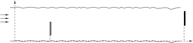
Figure 1: Illustration of the imaging setup in a waveguide with randomly perturbed boundary. The penetrable scatterer at range $z=L$ is illuminated by a partially coherent source. The detector at range $z=L+\mathcal{L}$ measures the spatially integrated energy flux of the waves, as a function of time.

Combining equations (1) and (2), we obtain that the pressure wave field is the solution of the wave equation

$$\Delta p(t,{{\itbf x}})-\frac{1}{c^{2}({{\itbf x}})}\partial_{t}^{2}p(t,{{\itbf x}})=e^{-i\omega_{o}t}f(t,x)\delta^{\prime}(z)+c.c.,$$ (6)

for $t\in\mathbb{R}$ and ${{\itbf x}}\in\big{(}\mathfrak{X}^{-}(z),\mathfrak{X}^{+}(z)\big{)}\times\mathbb{R}$, with Dirichlet boundary conditions

$$p(t,(x,z))=0,\quad x\in\{\mathfrak{X}^{-}(z),\mathfrak{X}^{+}(z)\},\,z\in\mathbb{R}.$$

The wave speed $c({{\itbf x}})$ is defined by

$$\frac{1}{c^{2}({{\itbf x}})}=\frac{1}{c_{o}^{2}}[1+{R}({{\itbf x}})\big{]},$$ (7)

where $c_{o}=\sqrt{K_{o}/\rho_{o}}$ is the constant wave speed in the homogeneous medium that fills the waveguide.

The cross-section of the waveguide is randomly fluctuating and has constant mean width $X$. We model the boundary by

$$\mathfrak{X}^{+}(z)=X\big{[}1+\sigma^{+}\mu^{+}(z)\big{]},\quad\mathfrak{X}^{-}(z)={X}\sigma^{-}\mu^{-}(z),$$ (8)

using the stationary random processes $\mu^{\pm}(z)$ with mean zero $\mathbb{E}[\mu^{\pm}(z)]=0$, where $\mathbb{E}[\cdot]$ denotes the expectation with respect to the statistical distribution of the random boundary fluctuations. The processes $\mu^{\pm}(z)$ may be independent or correlated and are mixing, with rapidly decaying mixing rate as defined in [8, Section 2]. Their autocorrelation

$$\mathcal{R}^{\pm}(z)=\mathbb{E}\big{[}\mu^{\pm}(z)\mu^{\pm}(0)\big{]},$$ (9)

is normalized to peak value $\mathcal{R}^{\pm}(0)=1$, and its integral

$$\int_{\mathbb{R}}{\rm d}z\,\mathcal{R}^{\pm}(z)=O(\ell),$$ (10)

defines the typical range scale of the fluctuations, the correlation length $\ell$. We assume as in [1] that $\mu^{\pm}(z)$ are twice continuously differentiable, with almost surely bounded derivatives, and quantify the standard deviation of the fluctuations of $\mathfrak{X}^{\pm}(z)$ using the small, positive and dimensionless parameters $\sigma^{\pm}\ll 1$.

The wave is generated by the random source (4) localized at $z=0$ and oriented in the range direction. The source signal is modulated at the carrier (central) frequency $\omega_{o}$ and has a slowly varying envelope $f(t,x)$. This is a complex-valued, stationary in time Gaussian process, with zero mean

$$\left<f(t,x)\right>=0,$$ (11)

zero relation function

$$\left<f(t,x)f(t^{\prime},x^{\prime})\right>=0,$$ (12)

and covariance

$$\left<f(t,x)\overline{f(t^{\prime},x^{\prime})}\right>=\sqrt{B}F\big{[}B(t-t^{\prime})]\theta(x,x^{\prime}).$$ (13)

The bar is used throughout the paper to denote complex conjugate and $\left<\cdot\right>$ denotes the expectation with respect to the distribution of the random source. The function $F$ in the expression of the covariance (13) is real valued, bounded, and integrable. The frequency scale $B$ in its argument is called the bandwidth, because it determines the support of the power spectral density function of $f(t,x)$, which is proportional to the Fourier transform of $F$ [9]. The real valued, integrable function $\theta(x,x^{\prime})$ models the spatial coherence of the source. It is supported in $\mathcal{A}_{\rm s}\times\mathcal{A}_{\rm s}$, where the interval $\mathcal{A}_{\rm s}\subseteq\big{(}\mathfrak{X}^{-}(0),\mathfrak{X}^{+}(0)\big{)}$ is called the source aperture. If the source is incoherent, then

$$\theta(x,x^{\prime})=\delta(x-x^{\prime})1_{\mathcal{A}_{\rm s}}(x),\quad~{}~{}1_{\mathcal{A}_{\rm s}}(x)=\left\{\begin{array}[]{ll}1,&x\in\mathcal{A}_{\rm s},\\ 0,&x\notin\mathcal{A}_{\rm s}.\end{array}\right.$$ (16)

The data for imaging the target are gathered at a detector located at range $z=L+\mathcal{L}$, with support (aperture) in the interval $\mathcal{A}_{\rm d}\subseteq\big{(}\mathfrak{X}^{-}(L+\mathcal{L}),\mathfrak{X}^{+}(L+\mathcal{L})\big{)}.$ In conventional imaging, the detector would measure the wave field $p(t,x,L+\mathcal{L}),$ for $t\in\mathbb{R}$ and $x\in\mathcal{A}_{\rm d}$, and the image would be formed using matched field [10] or reverse time migration processing [11, 12]. Such imaging is impeded by scattering at the random boundary of the waveguide. The long range cumulative effect of this scattering is described mathematically by the randomization of the wave and the energy exchange between its components, called the wave modes. This energy exchange is quantified by transport equations derived in [1] for waveguides with random boundaries, and in [13, Chapter 20] for waveguides filled with random media. Imaging based on these equations is studied in [14, 15].

None of the aforementioned imaging methods apply to the setting considered here, where the detector-target range offset $\mathcal{L}$ is so large that cumulative scattering distributes the energy evenly among the wave modes. It is not useful to measure $p(t,x,L+\mathcal{L})$ in this equipartition regime, so we consider instead measurements of the net energy flux through the detector

$$I(t)=\int_{\mathcal{A}_{\rm d}}{\rm d}x\,p(t,x,L+\mathcal{L}){\itbf e}_{z}\cdot{\itbf u}(t,x,L+\mathcal{L}),\quad t\in\mathbb{R}.$$ (17)

This flux, which is also called the sound power in the physical litterature [16], is associated with the usual energy density [13, Section 2.1.8]

$$e(t,x,z)=\frac{1}{2K_{o}}p(t,x,z)^{2}+\frac{\rho_{o}}{2}|{\itbf u}(t,x,z)|^{2}.$$

In spite of the limited data (17) and the strong scattering, we show that it is possible to image the target using a ghost-like imaging modality. Ghost imaging was introduced in the optics literature [17, 18, 19, 20] and was analyzed in the context of wave propagation in random media in [21]. The random source is realized in this context by a laser beam passed through a rotating glass diffuser [20], followed by a beam splitter that divides the beam in two parts: The first part illuminates the object of interest, which is typically a mask, and is then captured by a single pixel (bucket) detector. The second part does not interact with the mask and its time and spatially resolved energy flux is measured at a high resolution detector. The ghost image of the mask is then formed by correlation of the two energy flux measurements.

Here we have a different setting, where the whole source beam illuminates the target, which is not a mask, but a penetrable scatterer. The goal is to build an imaging modality for monitoring changes (i.e., emergence of targets) in the waveguide at $z=L$. If more than one range is of interest, then an image may be formed at each such range. The image is formed using the correlation of the data (17) with

$$I^{({\rm r})}(t,x)=p^{({\rm r})}(t,x,L){\itbf e}_{z}\cdot{\itbf u}^{({\rm r})}(t,x,L),$$ (18)

the energy flux at range $L$, in a reference waveguide (hence the superscript (r)), for the same wave source. We consider two reference waveguides:

1. The unperturbed waveguide, with straight boundary at $x=0$ and $x={X}$, where we can calculate $I^{({\rm r})}(t,x)$ analytically, provided we know the wave generated by the source. This implies either controlling the acoustic source or measuring the wave near the source.

2. The waveguide with the same random boundary (8), where $I^{({\rm r})}(t,x)$ must be measured before the presence of the target.

In either case, the imaging function at range $z=L$ is defined by

$$\mathscr{I}_{\tau,T}(x)=\int_{0}^{\tau}{\rm d}s\,\mathscr{C}_{T}(s,x),$$ (19)

where $\mathscr{C}_{T}$ is the empirical energy flux correlation

$$\mathscr{C}_{T}(s,x) = \frac{1}{T}\int_{0}^{T}{\rm d}t\,I^{({\rm r})}(t,x)\big{(}I(t+s)-I^{({\rm i})}(t+s)\big{)}-\Big{[}\frac{1}{T}\int_{0}^{T}{\rm d}t\,I^{({\rm r})}(t,x)\Big{]}$$ (20)

$$\times\Big{[}\frac{1}{T}\int_{0}^{T}{\rm d}t\,\big{(}I(t)-I^{({\rm i})}(t)\big{)}\Big{]}$$

and $I^{({\rm i})}(t)$ is the incident energy flux at the detector (hence the superscript (i)), in the absence of the target. This can be measured, or the terms involving it in (20) can be calculated in terms of the second-order statistics of the random processes $\mu^{\pm}(z)$.

The imaging function (19) is designed to reflect the transverse profile of the target at $z=L$. It is not the classical ghost imaging function used in optics [20], where the waves are monochromatic, there is no waveguide effect and one can simply evaluate $\mathscr{C}_{T}(s=0,x)$. Waveguides are dispersive, meaning that different components (modes) of the wave field propagate at different speed along the axis of the waveguide. Our analysis shows that due to mode dispersion, the imaging function should involve the integration of $\mathscr{C}_{T}(s,x)$ over the time lag $s$, in a time window of duration $\tau$ that is long enough to encompass the arrival of sufficiently many propagating modes.

More explicitly, we show that the two user defined parameters $\tau$ and $T$ affect the statistical stability and focusing of the imaging function (19) at the target. Statistical stability means that the image is approximately the same for all the realizations of the random source and boundary,

$$\mathscr{I}_{\tau,T}(x)\approx\mathbb{E}\big{[}\left<\mathscr{I}_{\tau,T}(x)\right>\big{]}.$$ (21)

We will see that the empirical correlation (20) converges as $T\to\infty$, in probability, to the statistical correlation with respect to the distribution of the random source. We will also see that for a large enough bandwidth $B$, the imaging function is insensitive to the realization of the fluctuations $\mu^{\pm}(z)$. Thus, to ensure a robust image, the wave field should not be monochromatic and the integration time $T$ should be large enough. Once the bandwidth is taken into account, the mode dispersion in the waveguide becomes important. The time parameter $\tau$ controls how many modes are used in the image formation and consequently, it determines the resolution of the image. At the very least, $\tau$ should satisfy the order relation

$$\frac{\mathcal{L}}{c_{o}}<\tau\ll T,$$ (22)

where the lower bound defines the travel time scale from the target to the detector. If we want all the propagating modes to contribute, it should satisfy

$$\frac{\mathcal{L}}{c_{o}}\ll\tau\ll T.$$ (23)

The goal of the paper is to analyze the imaging function (19). The analysis is based on the theory of wave propagation in random waveguides, developed in [1]. We quantify the resolution of the image in terms of the type of reference waveguide, the target range $L$, the apertures $\mathcal{A}_{\rm s}$ and $\mathcal{A}_{\rm d}$ of the source and detector, the partial coherence of the source, and the time parameter $\tau$.

The paper is organized as follows: We begin in section 2 with the mathematical model of long range wave propagation in random waveguides and the mathematical model of the measurements (17) and the reference energy flux (18). The results of the analysis of the imaging function (19) are in section 3 and the details of the calculations are given in appendices. We end with a summary in section 4.

2 Long range wave propagation in the random waveguide

In this section we summarize the wave propagation results obtained in [1]. As explained in [1, 12] these results are qualitatively (but not quantitatively) the same as those in waveguides filled with random media analyzed in [22, 23] and [13, Chapter 20]. We begin with the scaling regime in section 2.1. The mathematical model of the wave in the empty random waveguide, called the incident wave, is given in section 2.2. The model of the scattered wave is in section 2.3. We use it to derive the mathematical model of (17)–(18) in section 2.4.

2.1 Long range scaling

Let us introduce the small and positive dimensionless parameter $\varepsilon\ll 1$, which gives the order of magnitude of the standard deviation of the random fluctuations of the boundary in (8),

$$\sigma^{\pm}\sim\varepsilon,$$ (24)

where the symbol $\sim$ means that $\sigma^{\pm}/\varepsilon$ is bounded above and below by positive constants independent of $\varepsilon$.

The effect of these fluctuations depends on the relation between the correlation length $\ell$ and the carrier wavelength $\lambda_{o}=2\pi c_{o}/\omega_{o}$. We assume as in [1] that

$$\ell\sim\lambda_{o},$$ (25)

so there is an efficient interaction of the wave with the random boundary. Because the standard deviation (24) is small, this interaction has a negligible effect at small range,

$$p(t,{{\itbf x}})\approx p_{o}(t,{{\itbf x}}),\qquad z\sim\ell,$$ (26)

where $p_{o}(t,{{\itbf x}})$ is the solution of the wave equation in the unperturbed waveguide. However, the scattering effect accumulates as the wave propagates and becomes significant at $z\sim\ell/\varepsilon^{2}$. The wave $p(t,{{\itbf x}})$ is randomized at such ranges and it is quite different from $p_{o}(t,{{\itbf x}})$, as shown in [1].

We denote by $z_{\varepsilon}$ the range coordinate in this scaling, with the target and detector located at $z_{\varepsilon}=L_{\varepsilon}$ and $z_{\varepsilon}=L_{\varepsilon}+\mathcal{L}_{\varepsilon}$, where

$$\frac{\varepsilon^{2}L_{\varepsilon}}{\ell}\sim 1,\quad\frac{\varepsilon^{2}\mathcal{L}_{\varepsilon}}{\ell}\sim 1.$$ (27)

In an abuse of notation, we let

$$L_{\varepsilon}=\frac{L}{\varepsilon^{2}},\quad\mathcal{L}_{\varepsilon}=\frac{\mathcal{L}}{\varepsilon^{2}},$$ (28)

with $L$ and $\mathcal{L}$ independent of $\varepsilon$, satisfying

$$\frac{\mathcal{L}}{L}\gg 1,$$ (29)

which means that the target-detector distance is much larger than the source-target distance.

The mean width of the cross-section of the waveguide satisfies

$$\frac{{X}}{\lambda_{o}}\gg 1,\quad\mbox{independent of }\varepsilon,$$ (30)

so that the wave has many propagating components (modes). This is needed to achieve a good resolution of the image, as long as the time parameter $\tau$ in (19) is chosen appropriately. We rename this parameter $\tau_{\varepsilon}$, to emphasize its dependence on $\varepsilon$, and obtain from (21) and (27)–(29) that it should satisfy the scaling relation

$$\tau_{\varepsilon}=\frac{\mathfrak{T}}{\varepsilon^{2}},$$ (31)

with $\mathfrak{T}$ independent of $\varepsilon$. The other time parameter $T$, used in the calculation of the empirical correlation (20), is much larger than $\tau_{\varepsilon}$, so we can analyze the imaging function by taking first the limit $T\to\infty$ and then $\varepsilon\to 0$.

To have the same number of propagating modes at all the frequencies in the spectrum of the source, we take a small $\varepsilon$ dependent bandwidth denoted by $B_{\varepsilon}$,

$$\frac{B_{\varepsilon}}{\omega_{o}}\sim\varepsilon^{\alpha},\quad\alpha\in(1,2).$$ (32)

The choice $\alpha<2$ ensures that the covariance (13) is supported at time offsets $\sim 1/B_{\varepsilon}$ that are much smaller than the travel time of order $L_{\varepsilon}/c_{o}$ from the source to the target. Therefore, we may think of $F$ in (13) as a pulse. The choice $\alpha<2$ also gives the statistical stability of the image (19) with respect to the realizations of $\mu^{\pm}(z_{\varepsilon})$, as explained in section 3.2.1. The choice $\alpha>1$ is convenient because we can neglect some deterministic mode dispersion effects in the waveguide.

2.2 The incident wave

As is usual in scattering theory, we call the solution $p^{({\rm i})}(t,x,z_{\varepsilon})$ of the wave equation in the empty waveguide “the incident wave”, hence the index ${(i)}$. We write it using the Green’s function of the Helmholtz equation

$$\big{[}\Delta+k^{2}(\omega+\omega_{o})\big{]}\widehat{g}\big{(}\omega,(x,z_{\varepsilon}),(\xi,\zeta_{\varepsilon})\big{)}=\delta(x-\xi)\delta^{\prime}(z_{\varepsilon}-\zeta_{\varepsilon}),$$ (33)

at frequency offset $\omega$ from the carrier $\omega_{o}$, where $k(\omega+\omega_{o})=(\omega+\omega_{o})/c_{o}$ is the wavenumber. This Green’s function is bounded and outgoing at $|z_{\varepsilon}|\to\infty$ and defines the incident wave as

$$p^{({\rm i})}(t,x,z_{\varepsilon}) = \frac{1}{2\pi}\int_{-\infty}^{\infty}e^{-i(\omega+\omega_{o})t}\,{\rm d}\widehat{p}^{\,({\rm i})}(\omega,x,z_{\varepsilon})+c.c.,$$ (34)

$${\rm d}\widehat{p}^{\,({\rm i})}(\omega,x,z_{\varepsilon}) = \int_{\mathcal{A}_{\rm s}}\widehat{g}\big{(}\omega,(x,z_{\varepsilon}),(\xi,0)\big{)}{\rm d}\widehat{f}(\omega,\xi){\rm d}\xi.$$ (35)

In this expression we used the spectral theorem for stationary processes [9, Section 9.4] to represent $f(t,x)$ by the complex Gaussian measure ${\rm d}\widehat{f}(\omega,x)$ satisfying

$$\left<{\rm d}\widehat{f}(\omega,x)\right> = 0,$$ (36)

$$\left<{\rm d}\widehat{f}(\omega,x){\rm d}\widehat{f}(\omega^{\prime},x^{\prime})\right> = 0,$$ (37)

$$\left<{\rm d}\widehat{f}(\omega,x){\rm d}\overline{\widehat{f}(\omega^{\prime},x^{\prime})}\right> = \frac{2\pi}{\sqrt{B_{\varepsilon}}}\widehat{F}\Big{(}\frac{\omega}{B_{\varepsilon}}\Big{)}\theta(x,x^{\prime})\delta(\omega-\omega^{\prime}){\rm d}\omega{\rm d}\omega^{\prime}.$$ (38)

We call ${\rm d}\widehat{f}(\omega,x)$ the Fourier transform of $f(t,x)$, in an abuse of terminology. Note that $\widehat{F}$, the Fourier transform of $F$, is the power spectral density of a stationary process, so it is real valued and non-negative by Bochner’s theorem [9].

The Green’s function is given by a superposition of time harmonic waves (modes) which are either propagating or evanescent. The mode decomposition is obtained by expanding $\widehat{g}$ in the orthonormal basis $\big{(}\varphi_{j}(x)\big{)}_{j\geq 1}$ of the eigenfunctions

$$\varphi_{j}(x)=\sqrt{\frac{2}{{X}}}\sin\Big{(}\frac{\pi jx}{{X}}\Big{)}$$ (39)

of the operator $\partial_{x}^{2}$ with Dirichlet boundary conditions at $x=0$ and $x=X$. This expansion is justified because equation (33) can be rewritten in the unperturbed waveguide domain $(0,{X})\times\mathbb{R}$ with a change of variables that flattens the boundary and maps the fluctuations $\mu^{\pm}(z_{\varepsilon})$ to coefficients in the transformed Laplacian operator [1]. The expression of the Green’s function at $z_{\varepsilon}>\zeta_{\varepsilon}$ is

$$\widehat{g}(\omega,(x,z_{\varepsilon}),(\xi,\zeta_{\varepsilon})) \approx \sum_{j=1}^{N(\omega)}\varphi_{j}(x)\frac{a_{j}\big{(}\omega,z_{\varepsilon};(\xi,\zeta_{\varepsilon})\big{)}}{\sqrt{\beta_{j}(\omega+\omega_{o})}}e^{i\beta_{j}(\omega+\omega_{o})(z_{\varepsilon}-\zeta_{\varepsilon})}$$ (40)

$$+\sum_{j=N(\omega)+1}^{\infty}\varphi_{j}(x)\widehat{g}_{j}\big{(}\omega,z_{\varepsilon};(\xi,\zeta_{\varepsilon})\big{)},$$

where the approximation is because we neglect the backward propagating modes.

The first term in (40) sums the $N(\omega)$ forward propagating modes. With our choice (32) of the bandwidth we have $\omega\sim B_{\varepsilon}\sim\varepsilon^{\alpha}\omega_{o}$ and therefore,

$$N(\omega)=\left\lfloor\frac{k(\omega+\omega_{o}){X}}{\pi}\right\rfloor\approx N(\omega_{o}),\quad\mbox{for}~{}\varepsilon\ll 1,$$ (41)

where $\lfloor\cdot\rfloor$ denotes the integer part. We omit henceforth the argument $\omega_{o}$ of $N$, to simplify notation. The $j$th forward propagating mode in (40) is the combination of two plane waves

$$\varphi_{j}(x)e^{i\beta_{j}(\omega+\omega_{o})(z_{\varepsilon}-\zeta_{\varepsilon})}=-\frac{i}{\sqrt{2{X}}}\left[e^{i\boldsymbol{\kappa}_{j}^{+}\cdot(x,z_{\varepsilon}-\zeta_{\varepsilon})}-e^{i\boldsymbol{\kappa}_{j}^{-}\cdot(x,z_{\varepsilon}-\zeta_{\varepsilon})}\right],$$ (42)

that cancel each other at the boundary points $x=0$ and $x=X$. Their wave vectors

$$\boldsymbol{\kappa}_{j}^{\pm}=\big{(}\pm\frac{\pi j}{{X}},\beta_{j}(\omega+\omega_{o})\big{)}$$

have Euclidian norm $\|\boldsymbol{\kappa}_{j}^{\pm}\|=k(\omega+\omega_{o})$ and a positive component in the range direction, called the $j$th mode wavenumber,

$$\beta_{j}(\omega+\omega_{o})=\sqrt{k^{2}(\omega+\omega_{o})-\Big{(}\frac{\pi j}{{X}}\Big{)}^{2}}.$$ (43)

The backward propagating waves have a similar expression, except that their wave vectors have range components of opposite sign. Because we assume smooth random boundary fluctuations, we can use the forward scattering approximation which neglects these backward going waves. A detailed justification of this approximation is in [1] (see also [22] and [13, Chapter 20]).

The terms $\widehat{g}_{j}$ of the series in (40) are the evanescent modes, which decay exponentially with the range offset $z_{\varepsilon}-\zeta_{\varepsilon}$ and are negligible at the detector. However, they interact with the propagating modes over the long range of propagation, as described in [1]. This interaction is taken into account in the statistical description of the propagating mode amplitudes $a_{j}$. These are random fields with starting values

$$a_{j}\big{(}\omega,\zeta_{\varepsilon};(\xi,\zeta_{\varepsilon})\big{)}=\frac{\sqrt{\beta_{j}(\omega+\omega_{o})}}{2}\varphi_{j}(\xi),\quad j=1,\ldots,N,$$ (44)

and evolve at $z_{\varepsilon}>\zeta_{\varepsilon}$ as described by

$$\left(\begin{array}[]{c}a_{1}\big{(}\omega,z_{\varepsilon};(\xi,\zeta_{\varepsilon})\big{)}\\ \vdots\\ a_{N}\big{(}\omega,z_{\varepsilon};(\xi,\zeta_{\varepsilon})\big{)}\end{array}\right)={\bf P}(\omega,z_{\varepsilon};\zeta_{\varepsilon})\left(\begin{array}[]{c}a_{1}\big{(}\omega,\zeta_{\varepsilon};(\xi,\zeta_{\varepsilon})\big{)}\\ \vdots\\ a_{N}\big{(}\omega,\zeta_{\varepsilon};(\xi,\zeta_{\varepsilon})\big{)}\end{array}\right),$$ (51)

using the complex, random $N\times N$ propagator matrix ${\bf P}(\omega,z_{\varepsilon};\zeta_{\varepsilon})$. This matrix equals the identity at $z_{\varepsilon}=\zeta_{\varepsilon}$ and its statistics is described in the limit $\varepsilon\to 0$ in [1].

2.3 The scattered wave

The solution of the wave equation (6), with wave speed defined in (7)–(5), has the form

$$p(t,x,z_{\varepsilon})=\frac{1}{2\pi}\int_{-\infty}^{\infty}e^{-i(\omega+\omega_{o})t}\,{\rm d}\widehat{p}(\omega,x,z_{\varepsilon})+c.c.,$$ (52)

where ${\rm d}\widehat{p}$ satisfies the Lippmann-Schwinger equation

$${\rm d}\widehat{p}(\omega,x,z_{\varepsilon}) = {\rm d}\widehat{p}^{\,({\rm i})}(\omega,x,z_{\varepsilon})-k^{2}(\omega+\omega_{o})\int_{0}^{X}{\rm d}y\,{r}(y)\widehat{G}\big{(}\omega,(x,z_{\varepsilon}),(y,L_{\varepsilon})\big{)}$$ (53)

$$\times{\rm d}\widehat{p}(\omega,y,L_{\varepsilon}).$$

Here we introduced another Green’s function, satisfying the Helmholtz equation

$$\big{[}\Delta+k^{2}(\omega+\omega_{o})\big{]}\widehat{G}\big{(}\omega,(x,z_{\varepsilon}),(\xi,\zeta_{\varepsilon})\big{)}=\delta(x-\xi)\delta(z_{\varepsilon}-\zeta_{\varepsilon}).$$ (54)

This equation is like (33), except that there is no range derivative of the Dirac $\delta(z_{\varepsilon}-\zeta_{\varepsilon})$. The expression of $\widehat{G}$ is similar to (40),

$$\widehat{G}\big{(}\omega,(x,z_{\varepsilon}),(\xi,\zeta_{\varepsilon})\big{)}\approx\sum_{j=1}^{N}\varphi_{j}(x)\frac{A_{j}\big{(}\omega,z_{\varepsilon};(\xi,\zeta_{\varepsilon})\big{)}}{\sqrt{\beta_{j}(\omega+\omega_{o})}}e^{i\beta_{j}(\omega+\omega_{o})(z_{\varepsilon}-\zeta_{\varepsilon})},$$ (55)

where we neglected the evanescent modes. The random mode amplitudes $A_{j}$ are defined as in equation (51), by the same propagator ${\bf P}(\omega,z_{\varepsilon};\zeta_{\varepsilon})$, but their starting values are different,

$$A_{j}\big{(}\omega,\zeta_{\varepsilon};(\xi,\zeta_{\varepsilon})\big{)}=\frac{\varphi_{j}(\xi)}{2i\sqrt{\beta_{j}(\omega+\omega_{o})}},\quad j=1,\ldots,N.$$ (56)

The scattered wave

$$p^{({\rm s})}(t,x,z_{\varepsilon})=\frac{1}{2\pi}\int_{-\infty}^{\infty}e^{-i(\omega+\omega_{o})t}\,{\rm d}\widehat{p}^{\,({\rm s})}(\omega,x,z_{\varepsilon})+c.c.,$$ (57)

with Fourier transform

$${\rm d}\widehat{p}^{\,({\rm s})}(\omega,x,z_{\varepsilon})={\rm d}\widehat{p}(\omega,x,z_{\varepsilon})-{\rm d}\widehat{p}^{\,({\rm i})}(\omega,x,z_{\varepsilon}),$$ (58)

depends nonlinearly on the reflectivity ${r}(y)$ of the target, assumed small. In imaging it is common to use the Born approximation of this wave, obtained by replacing ${\rm d}\widehat{p}(\omega,y,L_{\varepsilon})$ with ${\rm d}\widehat{p}^{\,({\rm i})}(\omega,y,L_{\varepsilon})$ in the integrand in (53). The imaging function (19) depends quadratically on ${r}(y)$, so for consistency, we keep the second order terms in the Born series expansion of the scattered wave

$${\rm d}\widehat{p}^{\,({\rm s})}(\omega,x,z_{\varepsilon}) \approx -k^{2}(\omega+\omega_{o})\int_{0}^{X}{r}(y)\widehat{G}\big{(}\omega,(x,z_{\varepsilon}),(y,L_{\varepsilon})\big{)}{\rm d}\widehat{p}^{\,({\rm i})}(\omega,y,L_{\varepsilon}){\rm d}y$$ (59)

$$+k^{4}(\omega+\omega_{o})\int\int_{0}^{X}{r}(y){r}(y^{\prime})\widehat{G}\big{(}\omega,(x,z_{\varepsilon}),(y,L_{\varepsilon})\big{)}$$

$$\hskip 36.135pt\times\widehat{G}_{o}\big{(}\omega,(y,L_{\varepsilon}),(y^{\prime},L_{\varepsilon})\big{)}{\rm d}\widehat{p}^{\,({\rm i})}(\omega,y^{\prime},L_{\varepsilon}){\rm d}y{\rm d}y^{\prime}.$$

Here we replaced $\widehat{G}\big{(}\omega,(y,L_{\varepsilon}),(y^{\prime},L_{\varepsilon})\big{)}$ by the Green’s function in the unperturbed waveguide

$$\widehat{G}_{o}\big{(}\omega,(y,L_{\varepsilon}),(y^{\prime},L_{\varepsilon})\big{)}=\sum_{j=1}^{\infty}\frac{\varphi_{j}(y)\varphi_{j}(y^{\prime})}{2i\beta_{j}(\omega+\omega_{o})},$$ (60)

because the random boundary has a negligible effect on the wave propagation between the nearby points $(y,L_{\varepsilon})$ and $(y^{\prime},L_{\varepsilon})$ in the support of the target. The series in (60) involves both the propagating and the evanescent modes, with wavenumbers $\beta_{j}(\omega+\omega_{o})$ defined in (43) for $j=1,\ldots,N$, and with

$$\beta_{j}(\omega+\omega_{o})=i\sqrt{\Big{(}\frac{\pi j}{{X}}\Big{)}^{2}-k^{2}(\omega+\omega_{o})},\quad j>N.$$ (61)

2.4 The measurements and the reference energy flux

The detector measures the spatially integrated energy flux

$$I(t)=\int_{\mathcal{A}_{\rm d}}{\rm d}x\,p(t,x,L_{\varepsilon}+\mathcal{L}_{\varepsilon}){\itbf e}_{z}\cdot{\itbf u}(t,x,L_{\varepsilon}+\mathcal{L}_{\varepsilon}),$$ (62)

with $p(t,x,L_{\varepsilon}+\mathcal{L}_{\varepsilon})$ defined in equations (52), (57)–(59). These measurements are correlated in (19) with the energy flux

$$I^{({\rm r})}(t,x)=p^{({\rm r})}(t,x,L_{\varepsilon}){\itbf e}_{z}\cdot{\itbf u}^{({\rm r})}(t,x,L_{\varepsilon}),$$ (63)

of the wave, where

$$p^{({\rm r})}(t,x,L_{\varepsilon})=\frac{1}{2\pi}\int_{-\infty}^{\infty}\int_{\mathcal{A}_{\rm s}}e^{-i(\omega+\omega_{o})t}\widehat{g}^{\,({\rm r})}\big{(}\omega,(x,L_{\varepsilon}),(\xi,0)\big{)}{\rm d}\widehat{f}(\omega,\xi){\rm d}\xi,$$ (64)

and

$${\itbf e}_{z}\cdot{\itbf u}^{({\rm r})}(t,x,L_{\varepsilon})=\frac{1}{2\pi}\int_{-\infty}^{\infty}\int_{\mathcal{A}_{\rm s}}\frac{e^{-i(\omega+\omega_{o})t}}{i(\omega_{o}+\omega)}\partial_{z}\widehat{g}^{\,({\rm r})}\big{(}\omega,(x,L_{\varepsilon}),(\xi,0)\big{)}{\rm d}\widehat{f}(\omega,\xi){\rm d}\xi.$$ (65)

The expression of $p^{({\rm r})}(t,x,L_{\varepsilon})$ is similar to (35), except for the Green’s function $\widehat{g}^{\,({\rm r})}$ which models the wave propagation in the reference waveguide. The expression of ${\itbf e}_{z}\cdot{\itbf u}^{({\rm r})}(t,x,L_{\varepsilon})$ follows from (2) which reads in the Fourier domain as

$$-i\rho_{o}(\omega+\omega_{o}){\itbf e}_{z}\cdot{\rm d}\widehat{\itbf u}^{({\rm r})}(\omega,x,z_{\varepsilon})+\partial_{z}{\rm d}\widehat{p}^{({\rm r})}(\omega,x,z_{\varepsilon})=0.$$

We consider two reference waveguides: The unperturbed waveguide, where

$$\widehat{g}^{\,({\rm r})}\big{(}\omega,(x,L_{\varepsilon}),(\xi,0)\big{)}\approx\frac{1}{2}\sum_{j=1}^{N}\varphi_{j}(x)\varphi_{j}(\xi)e^{i\beta_{j}(\omega+\omega_{o})L_{\varepsilon}},$$ (66)

and the random, empty waveguide, where

$$\widehat{g}^{\,({\rm r})}\big{(}\omega,(x,L_{\varepsilon}),(\xi,0)\big{)}=\widehat{g}\big{(}\omega,(x,L_{\varepsilon}),(\xi,0)\big{)}$$

$$\hskip 67.21056pt\approx\frac{1}{2}\sum_{j,q=1}^{N}\sqrt{\frac{\beta_{q}(\omega_{o})}{\beta_{j}(\omega_{o})}}\varphi_{j}(x)\varphi_{q}(\xi){P}_{jq}(\omega,L_{\varepsilon};0)e^{i\beta_{j}(\omega+\omega_{o})L_{\varepsilon}}.$$ (67)

In both cases we neglect the evanescent modes, which have a very small contribution at the large range $L_{\varepsilon}$. The random mode amplitudes are written in (67) in terms of the entries ${P}_{jq}$ of the propagator, as in equations (44)–(51). Because $\omega/\omega_{o}\sim\varepsilon^{\alpha}$, with $\alpha\in(1,2)$, we approximate the mode wavenumbers in the amplitudes by their value at the carrier frequency. The phase in (66)–(67) is

$$\beta_{j}(\omega+\omega_{o})L_{\varepsilon}=\beta_{j}(\omega_{o})L_{\varepsilon}+\omega\beta^{\prime}_{j}(\omega_{o})L_{\varepsilon}+O\big{(}\varepsilon^{2(\alpha-1)}\big{)},$$ (68)

where

$$\frac{1}{\beta_{j}^{\prime}(\omega_{o})}=\Big{(}\frac{{\rm d}\beta_{j}(\omega+\omega_{o})}{{\rm d}\omega}\mid_{\omega=0}\Big{)}^{-1}=\frac{c_{o}\beta_{j}(\omega_{o})}{k_{o}},$$ (69)

is the $j$th mode speed, satisfying

$$0<\frac{1}{\beta_{N}^{\prime}(\omega_{o})}<\frac{1}{\beta_{N}^{\prime}(\omega_{o})}<\ldots<\frac{1}{\beta_{1}^{\prime}(\omega_{o})}<c_{o}.$$ (70)

We use throughout the notation $k_{o}=k(\omega_{o})=\omega_{o}/c_{o}$.

3 Analysis of the ghost imaging function

The imaging function (19) is defined by the time integral of the empirical correlation of the reference energy flux $I^{({\rm r})}(t,x)$ and the difference $I(t)-I^{({\rm i})}(t)$ of the net intensities at the detector. The subtraction of the net energy flux $I^{({\rm i})}(t)$ of the incident wave is so that the imaging function vanishes in the absence of the target. This energy flux could be measured in the empty waveguide or, if this is not feasible, its contribution to the imaging function can be estimated in terms of the second order statistics of the random boundary fluctuations $\mu^{\pm}(z_{\varepsilon})$, as explained in section 3.3.

The empirical energy flux correlation (20) converges in the limit $T\to\infty$, in probability, to its statistical expectation with respect to the distribution of the random source [24, Proposition 2.3]. Assuming a large integration time $T$, we obtain the approximation

$$\mathscr{C}_{T}(s,x)\approx\mathscr{C}(s,x)=\left<I^{({\rm r})}(t,x)\big{[}I(t+s)-I^{({\rm i})}(t+s)\big{]}\right>-\left<I^{({\rm r})}(t,x)\right>\left<I(t)-I^{({\rm i})}(t)\right>.$$ (71)

This expression is independent of $t$, because of the time stationarity of the source. We calculate it in A.

The imaging function is given by

$$\mathscr{I}_{\tau_{\varepsilon},T}(x)\approx\mathscr{I}_{\tau_{\varepsilon}}(x)=\int_{0}^{\tau_{\varepsilon}}{\rm d}s\,\mathscr{C}(s,x),$$ (72)

with $\tau_{\varepsilon}=\mathfrak{T}/\varepsilon^{2}$ scaled as in (31). Its expression

$$\mathscr{I}_{\frac{\mathfrak{T}}{\varepsilon^{2}}}(x)\approx\frac{2\mathfrak{T}}{(2\pi)^{2}\rho_{o}^{2}c_{o}^{2}B_{\varepsilon}}{\rm Re}\int_{-\infty}^{\infty}{\rm d}\omega\,\widehat{F}\Big{(}\frac{\omega}{B_{\varepsilon}}\Big{)}^{2}\int_{-\infty}^{\infty}{\rm d}h\,\mbox{sinc}\left(\frac{h\mathfrak{T}}{2}\right)e^{-ih\frac{\mathfrak{T}}{2}}$$

$$\times\int\int_{0}^{X}{\rm d}y{\rm d}y^{\prime}\Big{[}\mathscr{G}_{12}(\omega-\varepsilon^{2}h,y^{\prime},x)\mathscr{G}_{11}(\omega,y,x)+\overline{\mathscr{G}_{12}(\omega,y,x)}\overline{\mathscr{G}_{11}(\omega-\varepsilon^{2}h,y^{\prime},x)}\Big{]}$$

$$\times\Big{[}-2r(y)\mathscr{G}_{31}(\omega,\omega-\varepsilon^{2}h,y,y^{\prime})-2r(y^{\prime})\mathscr{G}_{32}(\omega,\omega-\varepsilon^{2}h,y,y^{\prime})$$

$$\quad+2k_{o}^{2}r(y)\int_{0}^{X}{\rm d}y^{\prime\prime}r(y^{\prime\prime})\mathscr{G}_{31}(\omega,\omega-\varepsilon^{2}h,y^{\prime\prime},y^{\prime})\widehat{G}_{o}\big{(}\omega,(y^{\prime\prime},L_{\varepsilon}),(y,L_{\varepsilon})\big{)}$$

$$\quad+2k_{o}^{2}r(y^{\prime})\int_{0}^{X}{\rm d}y^{\prime\prime}r(y^{\prime\prime})\mathscr{G}_{32}(\omega,\omega-\varepsilon^{2}h,y,y^{\prime\prime})\overline{\widehat{G}_{o}\big{(}\omega-\varepsilon^{2}h,(y^{\prime\prime},L_{\varepsilon}),(y^{\prime},L_{\varepsilon})\big{)}}$$

$$\quad+k_{o}^{2}r(y)r(y^{\prime})\mathscr{G}_{2}(\omega,\omega-\varepsilon^{2}h,y,y^{\prime})\Big{]}$$ (73)

is derived in A, where we recall that $\widehat{F}$ and ${r}$ are real valued. Here we introduced the notation

$$\mathscr{G}_{11}(\omega,y,x)=\int\int_{\mathcal{A}_{\rm s}}{\rm d}\xi{\rm d}\xi^{\prime}\,\theta(\xi,\xi^{\prime})\widehat{g}\big{(}\omega,(y,L_{\varepsilon}),(\xi,0)\big{)}\overline{\widehat{g}^{({\rm r})}\big{(}\omega,(x,L_{\varepsilon}),(\xi^{\prime},0)\big{)}},$$ (74)

$$\mathscr{G}_{12}(\omega,y^{\prime},x)=\int\int_{\mathcal{A}_{\rm s}}{\rm d}\xi{\rm d}\xi^{\prime}\,\theta(\xi,\xi^{\prime})\overline{\widehat{g}\big{(}\omega,(y^{\prime},L_{\varepsilon}),(\xi,0)\big{)}}(-i)\partial_{z}{\widehat{g}^{({\rm r})}\big{(}\omega,(x,L_{\varepsilon}),(\xi^{\prime},0)\big{)}},$$ (75)

$$\mathscr{G}_{2}(\omega,\omega^{\prime},y,y^{\prime})=\int_{\mathcal{A}_{\rm d}}{\rm d}x^{\prime}\,\widehat{G}\big{(}\omega,(x^{\prime},L_{\varepsilon}+\mathcal{L}_{\varepsilon}),(y,L_{\varepsilon})\big{)}i\partial_{z}\overline{\widehat{G}\big{(}\omega^{\prime},(x^{\prime},L_{\varepsilon}+\mathcal{L}_{\varepsilon}),(y^{\prime},L_{\varepsilon})\big{)}},$$ (76)

$$\mathscr{G}_{31}(\omega,\omega^{\prime},y,y^{\prime})=\int_{\mathcal{A}_{\rm d}}{\rm d}x^{\prime}\,\widehat{G}\big{(}\omega,(x^{\prime},L_{\varepsilon}+\mathcal{L}_{\varepsilon}),(y,L_{\varepsilon})\big{)}i\partial_{z}\overline{\widehat{g}\big{(}\omega^{\prime},(x^{\prime},L_{\varepsilon}+\mathcal{L}_{\varepsilon}),(y^{\prime},L_{\varepsilon})\big{)}},$$ (77)

and

$$\mathscr{G}_{32}(\omega,\omega^{\prime},y,y^{\prime})=\int_{\mathcal{A}_{\rm d}}{\rm d}x^{\prime}\,\widehat{g}\big{(}\omega,(x^{\prime},L_{\varepsilon}+\mathcal{L}_{\varepsilon}),(y,L_{\varepsilon})\big{)}i\partial_{z}\overline{\widehat{G}\big{(}\omega^{\prime},(x^{\prime},L_{\varepsilon}+\mathcal{L}_{\varepsilon}),(y^{\prime},L_{\varepsilon})\big{)}}.$$ (78)

We calculate next the imaging function (73) in both the unperturbed and random waveguide, in order to quantify its focusing in terms of the target range $L_{\varepsilon}$, the apertures $\mathcal{A}_{\rm s}$ and $\mathcal{A}_{\rm d}$, the source coherence function $\theta$ and the time parameter $\mathfrak{T}$.

3.1 Imaging in the unperturbed waveguide

The expression of the imaging function is derived in B. It is given by the formula (124) for an arbitrary integration time $\mathfrak{T}$. This $\mathfrak{T}$ does not play an important role in the support of the image, although it affects its magnitude at the target, but it must be larger than $\beta^{\prime}_{1}(\omega_{o})\mathcal{L}$, the scaled travel time of the fastest propagating mode from the target to the receiver. Otherwise, $\mathscr{I}_{\frac{\mathfrak{T}}{\varepsilon^{2}}}(x)\equiv 0$. In section 3.1.1 we give the expression of the imaging function for $\mathfrak{T}>\beta^{\prime}_{N}(\omega_{o})\mathcal{L},$ which is simpler and independent of $\mathfrak{T}$, and analyze in section 3.1.2 its focusing in terms of the source coherence and the source and detector apertures. The general function (124) is displayed in section 3.1.3 for the case of a point target.

3.1.1 The imaging function for a long integration time

The expression of the imaging function at $\mathfrak{T}>\beta^{\prime}_{N}(\omega_{o})\mathcal{L}$ is

$$\mathscr{I}(x)\approx\frac{k^{2}_{o}\|F\|^{2}}{32\rho_{o}^{2}c_{o}^{2}}\int\int_{0}^{X}{\rm d}y{\rm d}y^{\prime}\Big{[}\Phi_{{\bf S}0}(x,y)\Phi_{{\bf S}1}(x,y^{\prime})+\Phi_{{\bf S}1}(x,y)\Phi_{{\bf S}0}(x,y^{\prime})$$

$$\hskip 79.49744pt+2\sum_{\stackrel{{\scriptstyle j,j^{\prime}=1}}{{j\neq j^{\prime}}}}^{N}\beta_{j}(\omega_{o}){S}_{jj^{\prime}}^{2}\varphi_{j}(x)^{2}\varphi_{j^{\prime}}(y)\varphi_{j^{\prime}}(y^{\prime})\Big{]}$$

$$\times\Big{[}-2\int_{0}^{X}{\rm d}y^{\prime\prime}\,\Phi_{{\bf D}0}(y^{\prime},y^{\prime\prime})\Phi_{-1}(y,y^{\prime\prime}){r}(y)r(y^{\prime\prime})+\Phi_{{\bf D}-1}(y,y^{\prime}){r}(y){r}(y^{\prime})\Big{]},$$ (79)

where $\|F\|$ is the $L^{2}$ norm of $F$ and ${\bf S}$ and ${\bf D}$ are the $N\times N$ matrices with entries

$${S}_{jj^{\prime}}=\int\int_{\mathcal{A}_{\rm s}}{\rm d}\xi{\rm d}\xi^{\prime}\,\theta(\xi,\xi^{\prime})\varphi_{j}(\xi)\varphi_{j^{\prime}}(\xi^{\prime}),\qquad{D}_{jj^{\prime}}=\int_{\mathcal{A}_{\rm d}}{\rm d}x\,\varphi_{j}(x)\varphi_{j^{\prime}}(x),$$ (80)

that depend on the source and receiver apertures and the coherence function $\theta$ of the source. Here we introduced the sums $\Phi_{n}$, $\Phi_{{\bf S}n}$, $\Phi_{{\bf D}n}$ defined for $n\geq-1$ by

$$\Phi_{n}(x,y) = \sum_{j=1}^{N}\beta_{j}(\omega_{o})^{n}\varphi_{j}(x)\varphi_{j}(y),$$ (81)

$$\Phi_{{\bf S}n}(x,y) = \sum_{j=1}^{N}\beta_{j}(\omega_{o})^{n}{S}_{jj}\varphi_{j}(x)\varphi_{j}(y),$$ (82)

$$\Phi_{{\bf D}n}(x,y) = \sum_{j=1}^{N}\beta_{j}(\omega_{o})^{n}{D}_{jj}\varphi_{j}(x)\varphi_{j}(y).$$ (83)

Note that when the source is incoherent (delta-correlated) with $\theta$ defined in (16), and has full aperture $\mathcal{A}_{\rm s}=(0,X)$, then ${\bf S}$ is the identity matrix. Similarly, ${\bf D}$ equals the identity when $\mathcal{A}_{\rm d}=(0,X)$. In these ideal cases the sums (82)–(83) equal (81), and can be approximated using that $N\gg 1$ by the scaling assumption (30). Except very close to the boundaries $x,y\in\{0,X\}$ we have

$$\Phi_{-1}(x,y) \approx \frac{2}{\pi N}\sum_{l=1}^{N}\Big{[}1-\Big{(}\frac{l}{N}\Big{)}^{2}\Big{]}^{-\frac{1}{2}}\sin\Big{(}k_{o}x\frac{l}{N}\Big{)}\sin\Big{(}k_{o}y\frac{l}{N}\Big{)}$$ (84)

$$\approx \frac{1}{2}J_{0}\big{(}k_{o}(x-y)\big{)},$$

and similarly,

$$\Phi_{0}(x,y)\approx\frac{k_{o}}{\pi}{\rm sinc}(k_{o}|x-y|),\qquad\Phi_{1}(x,y)\approx\frac{k_{o}^{2}}{4}\frac{J_{1}(k_{o}|x-y|)}{k_{o}|x-y|},$$ (85)

where $J_{0}$ and $J_{1}$ are the Bessel function of the first kind and of orders $0$ and $1$. All these functions are peaked at $x=y$, as illustrated in Fig. 2.

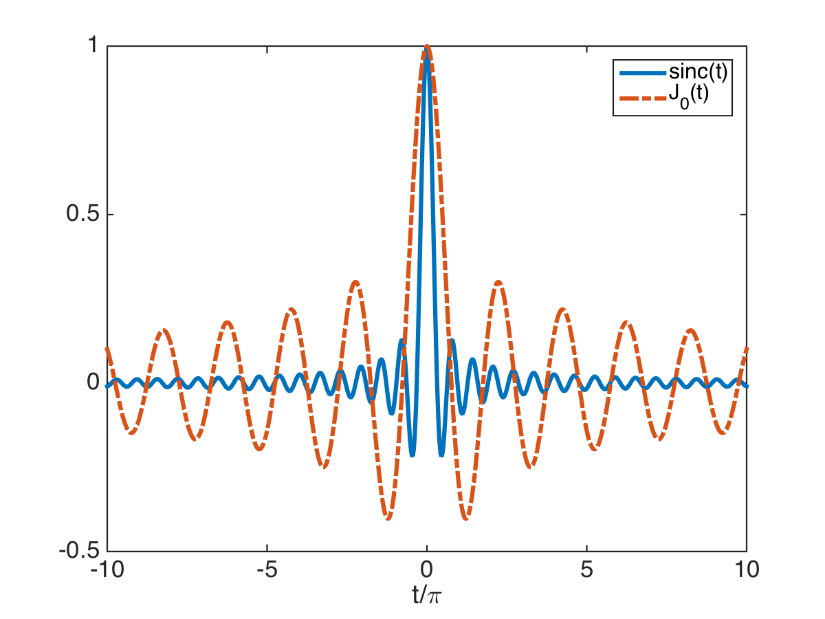
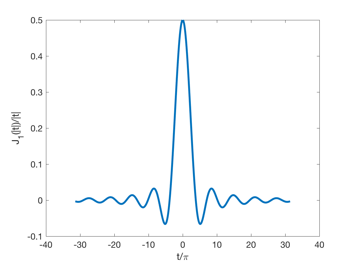
Figure 2: The Bessel functions which approximate $\Phi_{j}$, $j=-1,0,1$, as in (84-85). Left plot: the sinc function $\mbox{sinc}(t)$ (solid line) and the Bessel function $J_{0}(t)$ (dashed line) for $t\in[-10\pi,10\pi]$. Right plot: the function $\frac{J_{1}(|t|)}{|t|}$ for $t\in[-10\pi,10\pi]$ The argument $t$ is scaled by $\pi$ in the abscissa.

3.1.2 Quantification of resolution

The expression (79) shows that the imaging function is independent of the target range $L_{\varepsilon}=L/\varepsilon^{2}$.

The aperture $\mathcal{A}_{\rm d}$ of the detector, which defines the matrix ${\bf D}$, has a marginal role. For example, in the case $\mathcal{A}_{\rm d}=(0,a_{d})$, with $a_{d}\leq{X}$,

$${D}_{jj}=\int_{0}^{a_{d}}{\rm d}x^{\prime}\,\varphi_{j}^{2}(x^{\prime})=\frac{a_{d}}{{X}}\Big{[}1-\mbox{sinc}\Big{(}\frac{2j\pi a_{d}}{{X}}\Big{)}\Big{]}\approx\frac{a_{d}}{{X}},$$

where the approximation is for $j>{X}/a_{d}$. Thus, the functions $\Phi_{{\bf D}n}$ in (79) are approximately proportional to $\Phi_{n}$, for $n=-1,0$, and they give a similar contribution to the focus of the image for a full detector aperture or a smaller one.

The focusing of (79) at points $x$ in the support of the reflectivity ${r}$ is primarily dictated by the coupling matrix ${\bf S}$. The best focusing is for ${S}_{jj^{\prime}}=\delta_{jj^{\prime}}$, corresponding to an incoherent source with $\theta$ defined in (16) and a full aperture $\mathcal{A}_{\rm s}=(0,{X})$. The terms in $\sum_{j\neq j^{\prime}}$ in the square brackets in (79) vanish in this case and, if in addition the detector has full aperture, the imaging function becomes

$$\mathscr{I}(x)\approx-\frac{k^{2}_{o}\|F\|^{2}}{16\rho_{o}^{2}c_{o}^{2}}\int\int_{0}^{X}{\rm d}y{\rm d}y^{\prime}\,r(y)r(y^{\prime})\Phi_{0}(x,y)\Phi_{1}(x,y^{\prime})\Phi_{-1}(y,y^{\prime}).$$ (86)

The functions $\Phi_{n}$, for $n=-1,0,1$, are peaked at $x=y$ and are large for

$$|x-y|\leq\frac{\pi}{k_{o}}=\frac{\lambda_{o}}{2},$$

as seen from (84)–(85) and Fig. 2. Therefore, the image (79) focuses at $x$ in the support of the reflectivity ${r}$, with resolution $\lambda_{o}/2$. Note that $\mathscr{I}(x)$ has the form of a negative peak, which means that the target appears as a shadow.

If the source does not have full aperture or if it is partially coherent, then the imaging function remains focused at points in the support of ${r}$, as long as the matrix ${\bf S}$ is diagonally dominant. Otherwise, the terms in $\sum_{j\neq j^{\prime}}$ in the first square brackets in (79), which are not focused at points in the support of ${r}$, become significant.

3.1.3 Illustration of the point spread function

Here we illustrate the resolution analysis given above by displaying in Figure 3 the imaging function $\mathscr{I}(x)$ for a point target at cross-range $0.39X$, in a waveguide that supports $40$ propagating modes. We consider an incoherent source modeled as in (16), with $\mathcal{A}_{\rm s}=(0,a_{s})$, and a detector with aperture $\mathcal{A}_{\rm d}=(0,a_{d})$, for $0<a_{s},a_{d}\leq X$.

To illustrate the effect of the duration $\mathfrak{T}$ of the integration window, we display in Figure 3 the image $\mathscr{I}(x)$ calculated using the general formula (124), for three values of $\mathfrak{T}$: The first satisfies $\mathfrak{T}>\beta_{N}^{\prime}\mathcal{L}$, as assumed in the previous section, and the result is shown with the solid blue line. The other two satisfy $\beta_{n}^{\prime}\mathcal{L}<\mathfrak{T}<\beta_{n+1}^{\prime}\mathcal{L}$ for $n=10$ and $n=1$, and the results are shown with the dotted red line and the solid black line. We also illustrate the effect of the aperture of the source and detector by displaying the images for $a_{d}=X$ and $a_{s}=X,0.5X,0.1X$ in the top plots and for $a_{d}=0.5X,0.1X$ and $a_{s}=X$ in the bottom plots.

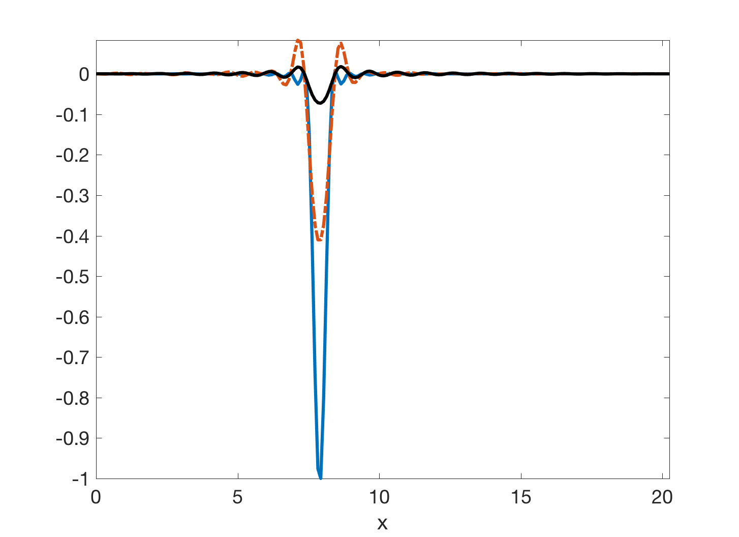
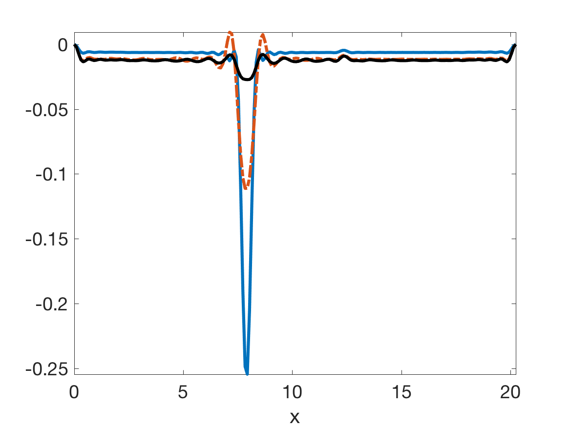
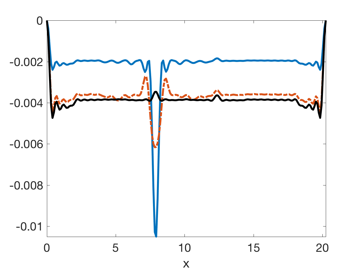
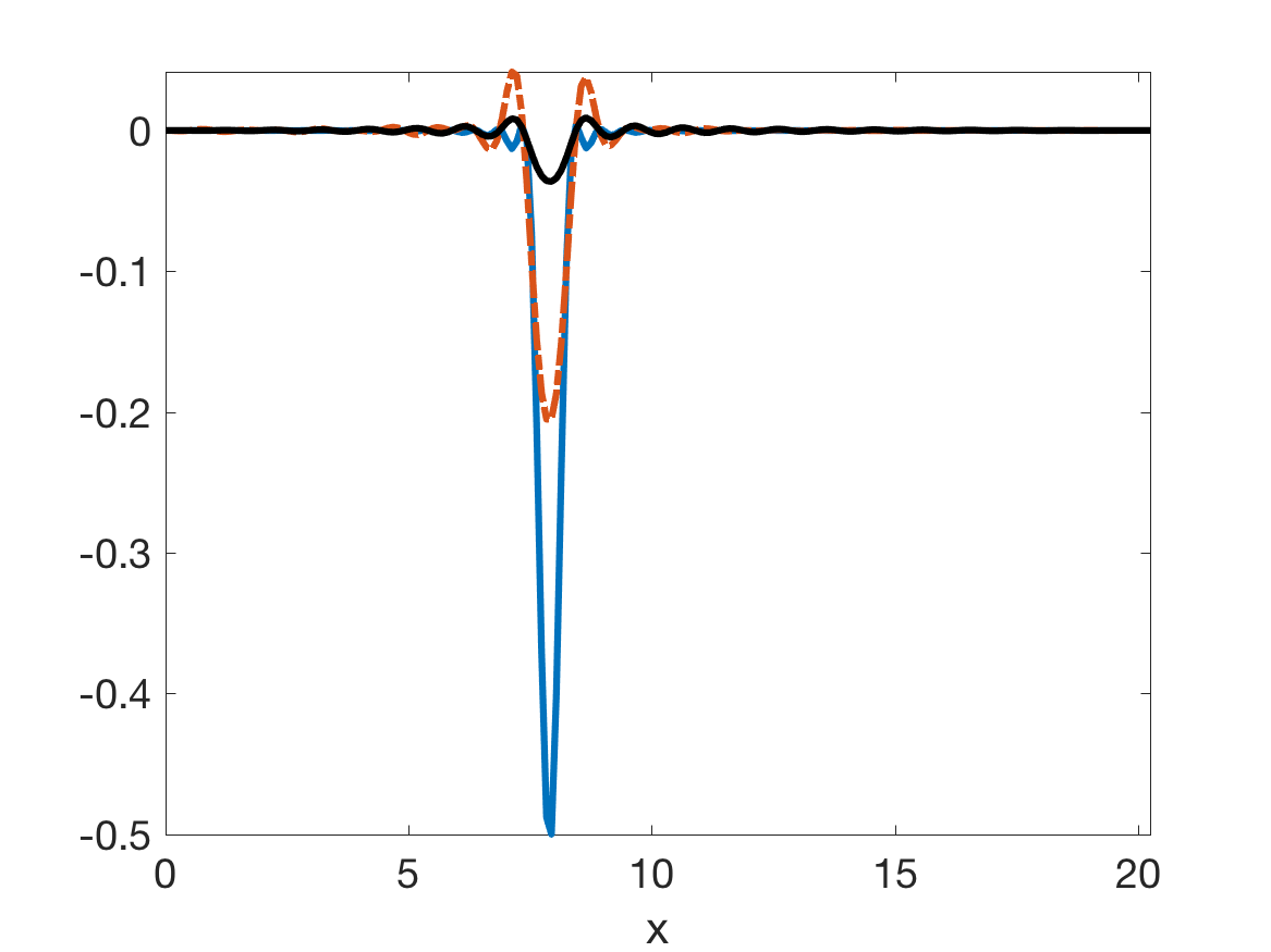
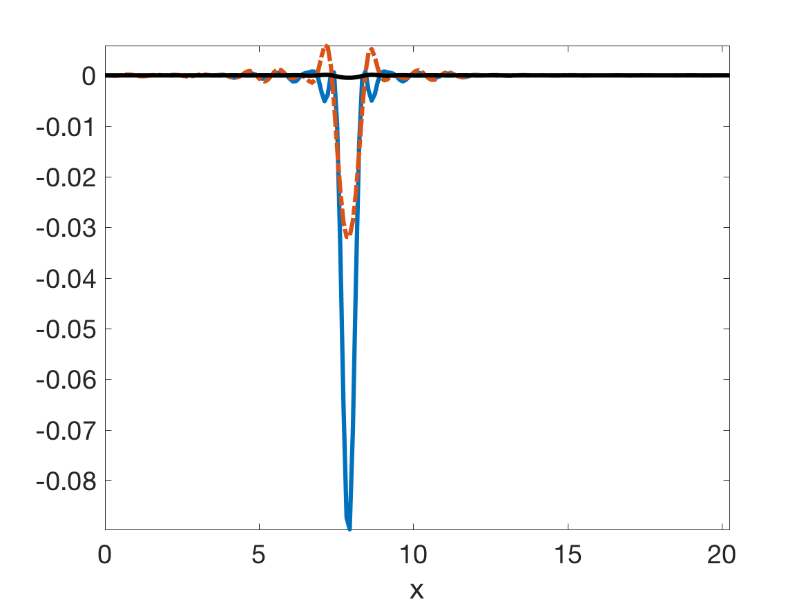
Figure 3: Imaging function (124) calculated for $\mathfrak{T}>\beta^{\prime}_{N}\mathcal{L}$ (79) (blue solid line) and $\beta_{n}^{\prime}\mathcal{L}<\mathfrak{T}<\beta_{n+1}^{\prime}\mathcal{L}$ for $n=10$ (red dotted line) and $n=1$ (black solid line). The top plots are for $a_{d}=X$ and, from left to right, $a_{s}=X,0.5X,0.1X$. The bottom plots are for $a_{s}=X$ and, from left to right, $a_{d}=0.5X,0.1X$. We normalize by the absolute value at the target location of the image calculated with $a_{d}=a_{s}=X$ and $\mathfrak{T}>\beta^{\prime}_{N}\mathcal{L}$. The abscissa is cross-range in units of the carrier wavelength.

As explained in the previous section, the image has a negative peak i.e., the target appears as a shadow at the true cross-range location $0.39X$. The value of $\mathfrak{T}$ has little effect on the support of this peak, but it affects its magnitude. The best results are for the large $\mathfrak{T}$, where the peak is more prominent and the side lobes are smaller.

The marginal effect of the detector aperture $a_{d}$ discussed in the previous section is seen in Figure 3 to consist of a multiplicative factor that makes the peak less prominent for the smaller $a_{d}$. However, the source aperture $a_{s}$ has a stronger effect on the image, which is no longer supported in the vicinity of the target location. At $50\%$ aperture (top middle plot) the value of the imaging function away from the target is small, but at $10\%$ aperture this value increases when compared to the peak and the target becomes less visible, especially for the smaller $\mathfrak{T}$.

3.2 Imaging in the random waveguide

We present here the analysis of the imaging function (73), in the waveguide with random boundary, using the unperturbed reference waveguide. To calculate $\mathscr{I}_{\frac{\mathfrak{T}}{\varepsilon^{2}}}(x)$, we recall from [1, 12] (see also [13, Chapter 20]) the relevant facts about the statistics of the wave propagator ${\bf P}(\omega,z_{\varepsilon};\zeta_{\varepsilon})$ in the limit $\varepsilon\to 0$:

1. The propagators ${\bf P}(\omega,z_{\varepsilon};\zeta_{\varepsilon})$ and ${\bf P}(\omega,z^{\prime}_{\varepsilon};\zeta^{\prime}_{\varepsilon})$ for any two non-overlapping range intervals $(z_{\varepsilon},\zeta_{\varepsilon})$ and $(z^{\prime}_{\varepsilon},\zeta_{\varepsilon}^{\prime})$ are uncorrelated.

2. The propagators ${\bf P}(\omega,z_{\varepsilon};\zeta_{\varepsilon})$ and ${\bf P}(\omega^{\prime},z_{\varepsilon};\zeta_{\varepsilon})$ for any two frequencies $\omega$ and $\omega^{\prime}$ satisfying $|\omega-\omega^{\prime}|\gg\varepsilon^{2}\omega_{o}$ are uncorrelated. Moreover,

   $${\bf P}(\omega,z_{\varepsilon};\zeta_{\varepsilon})\approx{\bf P}(\omega^{\prime},z_{\varepsilon};\zeta_{\varepsilon}),\quad\forall\omega,\omega^{\prime}\mbox{ satisfying }|\omega-\omega^{\prime}|\ll\varepsilon^{2}\omega_{o}.$$ (87)

3. The propagator satisfies the second moment formula

   $$\mathbb{E}\Big{[}{P}_{jq}(\omega,z_{\varepsilon};\zeta_{\varepsilon})\overline{{P}_{j^{\prime}q^{\prime}}(\omega-\varepsilon^{2}h,z_{\varepsilon};\zeta_{\varepsilon})}\Big{]}\to\delta_{jq}\delta_{j^{\prime}q^{\prime}}e^{\kappa_{jj^{\prime}}(z-\zeta)}$$

   $$\hskip 36.135pt+\delta_{jj^{\prime}}\delta_{qq^{\prime}}\int_{-\infty}^{\infty}{\rm d}t\,W_{j}^{(q)}(\omega_{o},t,z-\zeta)e^{ih\big{[}t-\beta_{j}^{\prime}(\omega_{o})(z-\zeta)\big{]}},$$ (88)

   where we let $z_{\varepsilon}=z/\varepsilon^{2}$, $\zeta_{\varepsilon}=\zeta/\varepsilon^{2}$ and used the symbol $\to$ to denote convergence in the limit $\varepsilon\to 0$.

The first term in the right-hand side of (88) models the energy of the coherent part of the wave. Its evolution in range is described by the complex matrix $(\kappa_{jj^{\prime}})$ given explicitly in [1] and [12, Section 6.2], in terms of the covariance of the random processes $\mu^{\pm}$. This matrix satisfies

$$\mbox{Re}[\kappa_{jj^{\prime}}]<0,\quad\kappa_{jj^{\prime}}=\overline{\kappa_{j^{\prime}j}},\quad\forall j,j^{\prime}=1,\ldots,N,$$ (89)

so the coherent term in (88) decays exponentially in range. The length scales $1/|\kappa_{jj}|$ of decay are called the scattering mean free paths of the modes. These scales are analyzed in [1] and decrease monotonically with the mode index $j$. The imaginary part of $(\kappa_{jj^{\prime}})$ vanishes on the diagonal, but it is non-zero otherwise. It accounts for dispersive effects due to scattering at the random boundary. The second term in (88) models the incoherent part of the energy, defined by the real valued, continuous density $W_{j}^{(q)}$ of the Wigner transform described in [12, Section 6.2] and [13, Proposition 20.7].

We consider a target at very long range offset from the detector, satisfying

$$\mathcal{L}\gg L_{\rm eq}\geq\frac{1}{|\kappa_{11}|},$$ (90)

where $L_{\rm eq}$ is the equipartition distance defined in [13, Section 20.3.3]. This is interesting because the wave reaching the detector is incoherent, meaning explicitly that

$$\mathbb{E}\big{[}\widehat{G}(\omega,(x,L_{\varepsilon}+\mathcal{L}_{\varepsilon}),(y,L_{\varepsilon})\big{]}\approx 0,~{}~{}\mathbb{E}\big{[}\widehat{g}(\omega,(x,L_{\varepsilon}+\mathcal{L}_{\varepsilon}),(y,L_{\varepsilon})\big{]}\approx 0,~{}~{}\forall x,y\in(0,X).$$ (91)

Moreover, the strong scattering in the range interval $z\in(L_{\varepsilon},L_{\varepsilon}+\mathcal{L}_{\varepsilon})$ distributes the energy evenly between the modes, independent of their amplitudes at the target. This makes conventional imaging impossible, but as we explain in section 3.2.2, the target can still be located with the ghost imaging modality.

3.2.1 Statistical stability

In (73) we integrate over the frequency $\omega$, which is of the order of the bandwidth $B_{\varepsilon}$, scaled as in (32). The propagator decorrelates over frequency offsets of order $\varepsilon^{2}\omega_{o}$ (item 2. above), so we integrate over many frequency decorrelation intervals and obtain by the law of large numbers the statistical stability result

$$\mathscr{I}_{\frac{\mathfrak{T}}{\varepsilon^{2}}}(x)\approx\mathbb{E}\Big{[}\mathscr{I}_{\frac{\mathfrak{T}}{\varepsilon^{2}}}(x)\Big{]}.$$ (92)

Note that the integration over $s\in(0,\tau_{\varepsilon})$ in (73), with $\tau_{\varepsilon}=\mathfrak{T}/\varepsilon^{2}$, ensures that the imaging function is given by the superposition of products of two Green’s functions (one with a complex conjugate) at frequencies $\omega$ and $\omega-\varepsilon^{2}h$, with $h\sim\omega_{o}$. The result (92) holds because the expectation in the right hand side is not small. If we did not integrate over $s$ in (73), or we had a much smaller $\tau_{\varepsilon}$, then the integrand would consist of products of uncorrelated Green’s functions, at frequencies offset by more than order $\varepsilon^{2}\omega_{o}$. The expectation of such products is given by the product of the expectations of the Green’s functions, which are negligible as in (91). The expectation of the terms in the integrand in (73) involve the second moments of the wave, which are not small, and this is why we obtain the result (92).

When calculating the expectation of (73) we note that $(\mathscr{G}_{1n})_{n=1,2}$ depend on the range section $(0,L_{\varepsilon})$ of the waveguide, whereas $\mathscr{G}_{2}$ and $(\mathscr{G}_{3n})_{n=1,2}$ depend on the range section $(L_{\varepsilon},L_{\varepsilon}+\mathcal{L}_{\varepsilon})$. By item 1. above, $\mathscr{G}_{11}$ and $\mathscr{G}_{12}$ are uncorrelated from $\mathscr{G}_{2}$, $\mathscr{G}_{31}$, and $\mathscr{G}_{32}$, so to approximate (73) we need the expectations of (76)–(78) and $\mathbb{E}\Big{[}\mathscr{G}_{11}(\omega,y,x){\mathscr{G}_{12}(\omega-\varepsilon^{2}h,y^{\prime},x)}\Big{]}$.

We consider large integration times $\mathfrak{T}\gg\mathcal{L}/c_{o}$ so that, as in the homogeneous case, the integral in $h$ in (73) becomes concentrated at $h=0$ and the imaging function becomes independent of $\mathfrak{T}$. As a consequence, we get from (73):

$$\mathscr{I}(x)\approx\frac{1}{\pi\rho_{o}^{2}c_{o}^{2}B_{\varepsilon}}{\rm Re}\int_{-\infty}^{\infty}{\rm d}\omega\,\widehat{F}\Big{(}\frac{\omega}{B_{\varepsilon}}\Big{)}^{2}\int\int_{0}^{X}{\rm d}y{\rm d}y^{\prime}$$

$$\times\mathbb{E}\Big{[}\mathscr{G}_{12}(\omega,y^{\prime},x)\mathscr{G}_{11}(\omega,y,x)+\overline{\mathscr{G}_{12}(\omega,y,x)}\overline{\mathscr{G}_{11}(\omega,y^{\prime},x)}\Big{]}$$

$$\times\Big{[}-2r(y)\mathbb{E}[\mathscr{G}_{31}(\omega,\omega,y,y^{\prime})]-2r(y^{\prime})\mathbb{E}[\mathscr{G}_{32}(\omega,\omega,y,y^{\prime})]$$

$$\quad+2k_{o}^{2}r(y)\int_{0}^{X}{\rm d}y^{\prime\prime}r(y^{\prime\prime})\mathbb{E}[\mathscr{G}_{31}(\omega,\omega,y^{\prime\prime},y^{\prime})]\widehat{G}_{o}\big{(}\omega,(y^{\prime\prime},L_{\varepsilon}),(y,L_{\varepsilon})\big{)}$$

$$\quad+2k_{o}^{2}r(y^{\prime})\int_{0}^{X}{\rm d}y^{\prime\prime}r(y^{\prime\prime})\mathbb{E}[\mathscr{G}_{32}(\omega,\omega,y,y^{\prime\prime})]\overline{\widehat{G}_{o}\big{(}\omega,(y^{\prime\prime},L_{\varepsilon}),(y^{\prime},L_{\varepsilon})\big{)}}$$

$$\quad+k_{o}^{2}r(y)r(y^{\prime})\mathbb{E}[\mathscr{G}_{2}(\omega,\omega,y,y^{\prime})]\Big{]}.$$ (93)

3.2.2 The imaging function

The expression of the imaging function is given in (136) for an arbitrary scaled range offset $L$ between the source and target. Here we write it in the two extreme cases, where the formulas are simpler:
1) For weak scattering i.e., $L$ smaller than the scattering mean free path of all the propagating modes, the imaging function has the form

$$\mathscr{I}(x)\approx\frac{k^{2}_{o}\|F\|^{2}C_{{\bf D}}}{32\rho_{o}^{2}c_{o}^{2}}\int\int_{0}^{X}{\rm d}y{\rm d}y^{\prime}\Big{[}\Phi_{{\bf S}0}(x,y)\Phi_{{\bf S}1}(x,y^{\prime})+\Phi_{{\bf S}1}(x,y)\Phi_{{\bf S}0}(x,y^{\prime})$$

$$\hskip 28.90755pt+2\sum_{j\neq j^{\prime}}\beta_{j}(\omega_{o}){S}_{jj^{\prime}}^{2}\varphi_{j}(x)^{2}\varphi_{j^{\prime}}(y)\varphi_{j^{\prime}}(y^{\prime})\Big{]}$$

$$\times\Big{[}-2r(y)\int_{0}^{X}{\rm d}y^{\prime\prime}r(y^{\prime\prime})\Phi_{0}(y^{\prime},y^{\prime\prime})\Phi_{-1}(y,y^{\prime\prime})+\Phi_{-1}(y,y^{\prime}){r}(y){r}(y^{\prime})\Big{]},$$ (94)

where

$$C_{{\bf D}}=\frac{1}{N}\sum_{m=1}^{N}{D}_{mm}=\frac{1}{N}\int_{\mathcal{A}_{\rm d}}\Phi_{0}(x^{\prime},x^{\prime}){\rm d}x^{\prime}.$$ (95)

2) When scattering is strong between the source and the target i.e., $L$ is larger than the scattering mean free path of all the propagating modes, the imaging function has the form

$$\mathscr{I}(x)\approx\frac{k^{2}_{o}\|F\|^{2}C_{{\bf D}}}{16\rho_{o}^{2}c_{o}^{2}}\int\int_{0}^{X}{\rm d}y{\rm d}y^{\prime}\Big{[}\sum_{j,j^{\prime},l=1}^{N}{S}_{j^{\prime}l}^{2}\varphi_{l}(x)^{2}\varphi_{j}(y)\varphi_{j}(y^{\prime})\frac{\beta_{j^{\prime}}(\omega_{o})\beta_{l}(\omega_{o})}{\beta_{j}(\omega_{o})}$$

$$\hskip 97.56493pt\times\int_{-\infty}^{\infty}{\rm d}t\,W_{j}^{(j^{\prime})}(\omega_{o},t,L)\Big{]}$$

$$\times\Big{[}-2r(y)\int_{0}^{X}{\rm d}y^{\prime\prime}r(y^{\prime\prime})\Phi_{0}(y^{\prime},y^{\prime\prime})\Phi_{-1}(y,y^{\prime\prime})+\Phi_{-1}(y,y^{\prime}){r}(y){r}(y^{\prime})\Big{]}.$$ (96)

Moreover, when $L$ exceeds the equipartition distance, the Wigner transform becomes independent of the indexes $j,j^{\prime}=1,\ldots,N$ and satisfies

$$\int_{-\infty}^{\infty}{\rm d}t\,W_{j}^{(j^{\prime})}(\omega_{o},t,L)\approx\frac{1}{N},\quad L\gg L_{\rm eq}.$$

As we explain below, the source aperture and coherence determine the focusing of the image in the weak scattering regime. In the strong scattering regime, the image is not focused at the target, even in the ideal case of an incoherent source with full aperture. Intermediate scattering regimes are an interpolation of these two extreme cases and the image focuses at the target when $L$ is smaller than the scattering mean free paths of sufficiently many modes.

3.2.3 Quantification of resolution

Note that the size of the detector appears only in the constant amplitude factor $C_{{\bf D}}$, so the focusing of the image is entirely dependent on the source and the target range $L$.

In the weak scattering regime (between the source and the target), the best result is obtained for an incoherent (delta-correlated) source that spans the entire cross section of the waveguide. The matrix ${\bf S}$ equals the identity in this case and (94) becomes

$$\mathscr{I}(x)\approx-\frac{k_{o}^{2}\|F\|^{2}C_{{\bf D}}}{16\rho_{o}^{2}c_{o}^{2}}\int\int_{0}^{X}{\rm d}y{\rm d}y^{\prime}r(y)r(y^{\prime})\Phi_{0}(x,y)\Phi_{1}(x,y^{\prime})\Phi_{-1}(y,y^{\prime}).$$ (97)

This is proportional to the imaging function (86) in the homogeneous waveguide, at full detector aperture. This shows that the strong wave scattering between the target and the detector is beneficial and removes the marginal effect of a limited detector aperture $\mathcal{A}_{\rm d}$ on the focusing of the image that we had observed in a homogeneous waveguide in sections 3.1.2–3.1.3. The image has a negative peak and has a resolution of order $\lambda_{o}/2$, as illustrated in the top left plot of Figure 3.

In the strong scattering regime between the source and the target, the image does not focus, no matter what the source aperture and coherence are. More precisely, in the ideal case of a delta-correlated source with full aperture, and for $L>L_{\rm eq}$, the expression (96) becomes

$$\mathscr{I}(x)\approx-\frac{k_{o}^{2}\|F\|^{2}C_{{\bf D}}}{16N\rho_{o}^{2}c_{o}^{2}}\Phi_{2}(x,x)\int\int_{0}^{X}{\rm d}y{\rm d}y^{\prime}r(y)r(y^{\prime})\Phi_{-1}(y,y^{\prime})^{2}.$$ (98)

This is approximately constant for $x$ away from the boundary points $0$ and $X$, as illustrated in the top left plot in Figure 4.

3.3 Contribution of the incident energy flux to the image

In case that $I^{({\rm i})}(t)$ cannot be measured, we show here that it is possible to estimate its contribution to the imaging function

$$\mathscr{I}^{({\rm i})}_{\frac{\mathfrak{T}}{\varepsilon^{2}}}(x) =\int_{0}^{\mathfrak{T}/\varepsilon^{2}}{\rm d}s\Big{[}\left<I^{({\rm r})}(t,x)I^{({\rm i})}(t+s)\right>-\left<I^{({\rm r})}(t,x)\right>\left<I^{({\rm i})}(t+s)\right>\Big{]}.$$ (99)

We calculate this expression in D and obtain that, for $\mathfrak{T}\gg\mathcal{L}/c_{o}$, (99) becomes independent of $\mathfrak{T}$ and has the form

$$\mathscr{I}^{({\rm i})}(x)\approx\frac{{C}_{{\bf D}}\|F\|^{2}}{8\rho_{o}^{2}c_{o}^{2}k_{o}^{2}}\Big{[}\sum_{j=1}^{N}{S}^{2}_{jj}\varphi_{j}(x)^{2}\beta_{j}(\omega_{o})^{2}e^{\kappa_{jj}L}+\sum_{\stackrel{{\scriptstyle j,l=1}}{{j\neq l}}}^{N}{S}_{jl}^{2}\varphi_{l}(x)^{2}\beta_{j}(\omega_{o})\beta_{l}(\omega_{o})e^{\kappa_{jj}L}$$

$$\quad\quad+\sum_{j,j^{\prime},l=1}^{N}{S}_{j^{\prime}l}^{2}\varphi_{l}(x)^{2}\beta_{j^{\prime}}(\omega_{o})\beta_{l}(\omega_{o})\int_{-\infty}^{\infty}{\rm d}t\,W_{j}^{(j^{\prime})}(\omega_{o},t,L)\Big{]}.$$ (100)

This is approximately constant in $x$, at least for ${\bf S}$ diagonally dominant, which is needed for the imaging function to focus at the target.

More explicitly, in the case of an incoherent source with full aperture, where ${\bf S}$ equals the identity matrix, we have in the weak scattering regime that

$$\mathscr{I}^{({\rm i})}(x)\approx\frac{{C}_{{\bf D}}\|F\|^{2}}{8\rho_{o}^{2}c_{o}^{2}k_{o}^{2}}\Phi_{2}(x,x).$$ (101)

Furthermore, in the strong scattering regime, at range $L\gg L_{\rm eq}$, we obtain exactly the same expression. Thus, the function $\mathscr{I}^{({\rm i})}(x)$ is proportional to $\Phi_{2}(x,x)$ and is approximately constant for $x$ away from the boundary points $0$ and $X$.

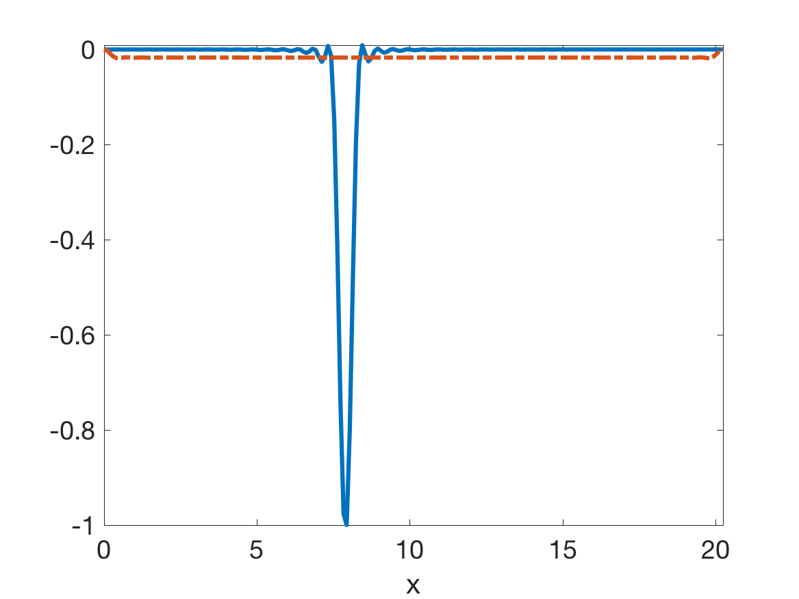
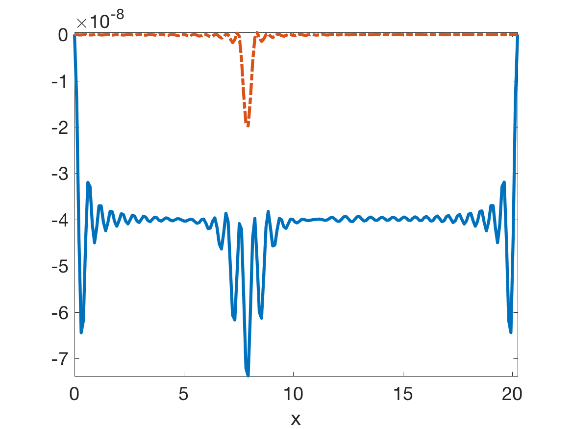
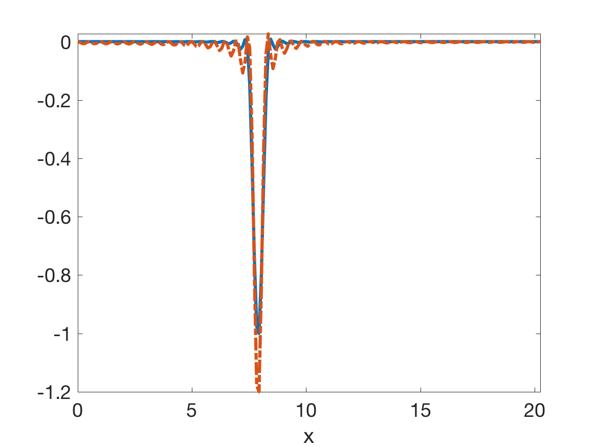
Figure 4: Left: Imaging function in the homogeneous waveguide (solid blue line) and in the random waveguide (where we cannot measure, so the reference waveguide is the homogeneous waveguide) (red dotted line) for full detector and full source aperture and for $\mathfrak{T}>\beta^{\prime}_{N}\mathcal{L}$. Middle: Imaging function in the homogeneous waveguide for all the recorded modes (solid line) and in the random waveguide (where we measure, so the reference waveguide is the same random waveguide) (red dotted line) for $a_{d}=a_{s}=0.05X$ and for $\mathfrak{T}>\beta^{\prime}_{N}\mathcal{L}$. Right: The same as in the middle, but for $a_{d}=a_{s}=X$. We normalize by the absolute value at the target location of the image calculated in the homogeneous waveguide, with $a_{d}=a_{s}=X$ and $\mathfrak{T}>\beta^{\prime}_{N}\mathcal{L}$. The abscissa is cross-range in units of the carrier wavelength.

3.4 Imaging based on the random reference waveguide

We present here the analysis of the imaging function (73), in the waveguide with random boundary, using the random waveguide as the reference waveguide. The imaging function is given by (73) but with $\mathscr{G}_{11}$ replaced by

$$\mathscr{G}_{11}(\omega,y,x)=\int\int_{\mathcal{A}_{\rm s}}{\rm d}\xi{\rm d}\xi^{\prime}\,\theta(\xi,\xi^{\prime})\widehat{g}\big{(}\omega,(y,L_{\varepsilon}),(\xi,0)\big{)}\overline{\widehat{g}\big{(}\omega,(x,L_{\varepsilon}),(\xi^{\prime},0)\big{)}},$$ (102)

and $\mathscr{G}_{12}$ replaced by

$$\mathscr{G}_{12}(\omega,y^{\prime},x)=\int\int_{\mathcal{A}_{\rm s}}{\rm d}\xi{\rm d}\xi^{\prime}\,\theta(\xi,\xi^{\prime})\overline{\widehat{g}\big{(}\omega,(y^{\prime},L_{\varepsilon}),(\xi,0)\big{)}}(-i)\partial_{z}{\widehat{g}\big{(}\omega,(x,L_{\varepsilon}),(\xi^{\prime},0)\big{)}}.$$ (103)

If the medium is weakly scattering between the source and the target, there is no difference compared to the case addressed in Section 3.2 and we find that the imaging function has the form (94). In this case, the quality of the image depends strongly of the source, as illustrated in Figure 3.

If the medium is strongly scattering between the source and the target, in the sense that $L$ is larger than the equipartition distance, then the situation is dramatically different from the one addressed in Section 3.2. As shown in E, we find that the imaging function has the form:

$$\mathscr{I}(x)\approx-\frac{k^{2}_{o}\|F\|^{2}C_{{\bf D}}C_{{\bf S}}}{16\rho_{o}^{2}c_{o}^{2}}\int\int_{0}^{X}{\rm d}y{\rm d}y^{\prime}{r}(y){r}(y^{\prime})\Phi_{-1}(x,y)\Phi_{0}(x,y^{\prime})\Phi_{-1}(y,y^{\prime}),$$ (104)

where $C_{{\bf D}}$ is given by (95) and $C_{{\bf S}}$ is defined by

$$C_{{\bf S}}=\frac{\big{[}\sum_{j=1}^{N}S_{jj}\beta_{j}(\omega_{o})\big{]}^{2}}{N(N+1)}=\frac{1}{N(N+1)}\Big{[}\int\int_{\mathcal{A}_{\rm s}}\theta(\xi,\xi^{\prime})\Phi_{1}(\xi,\xi^{\prime}){\rm d}\xi{\rm d}\xi^{\prime}\Big{]}^{2}.$$ (105)

In this case the source can be quite arbitrary. Its diameter and its coherence properties only affect the value of the constant $C_{{\bf S}}$. This robustness comes from the randomness of the medium that generates the suitable illumination. This result shows that we get an image (of the shadow) of the target, whatever the source and detector are and that the resolution is of order $\lambda_{o}/2$. The only effect of the apertures is in the multiplying constants $C_{{\bf D}}$ and $C_{{\bf S}}$ which should be large enough to make the peak observable in practice. This is illustrated in the middle and right plots in Figure 4, for the waveguide supporting $40$ propagating modes and the point target at cross-range $0.39X$.

4 Summary

We analyzed a ghost imaging modality in a waveguide with random boundary, for a penetrable scatterer (target) located between a partially coherent source and a detector that measures the energy flux. We considered a very large distance between the target and the detector, so that cumulative scattering of the waves at the random boundary distributes the energy evenly among the propagating components (modes) of the wave. Conventional imaging fails in this equipartition regime, but ghost imaging is possible in three configurations:
1) The source has large aperture (spans almost the entire cross-section of the waveguide) and is spatially delta-correlated, the waveguide is homogeneous, and we correlate the energy flux recorded at the detector with the spatially-resolved energy flux at the target distance in a reference homogeneous waveguide. The spatially-resolved energy flux in the reference homogeneous waveguide can be computed provided the source transmission is known because the waveguide modes are known. If the detector is large enough, imaging is possible and this is the classical ghost imaging situation.
2) The source has large aperture and is delta-correlated, the waveguide is random, and we correlate the energy flux recorded at the detector with the spatially-resolved energy flux at the target distance in a reference homogeneous waveguide. Ghost imaging is possible if scattering from the source to the target is weak. In this configuration, scattering between the target and the detector helps as it distributes the information over all the modes and the image becomes essentially independent of the aperture of the detector.
3) The source and the detector are arbitrary, the waveguide is random, and we correlate the energy flux recorded at the detector with the spatially-resolved energy flux at the target distance in the same random waveguide, used as the reference waveguide. The spatially-resolved energy flux in the reference waveguide cannot be computed because we do not know the realization of the random medium, so it needs to be measured, or one needs to measure the transmission matrix from the source plane to the target plane and to know the source transmission. Ghost imaging is then possible even if scattering from the source to the target and from the target to the detector is strong. This is in fact the optimal situation from the ghost imaging point of view, but it requires calibration i.e., measuring the energy flux in the waveguide in the absence of the target.

Appendix A Calculation of the energy flux correlation

The calculation of the correlation (71) of the energy flux is based on the expressions (35), (59), (62–65), the fourth-order moment formula

$$\left<{\rm d}\widehat{f}(\omega_{1},x_{1}){\rm d}\overline{\widehat{f}(\omega_{1}^{\prime},x_{1}^{\prime})}{\rm d}\overline{\widehat{f}(\omega_{2},x_{2})}{\rm d}\widehat{f}(\omega_{2}^{\prime},x_{2}^{\prime})\right>$$

$$~{}~{}-\left<{\rm d}\widehat{f}(\omega_{1},x_{1}){\rm d}\overline{\widehat{f}(\omega_{1}^{\prime},x_{1}^{\prime})}\right>\left<{\rm d}\overline{\widehat{f}(\omega_{2},x_{2})}{\rm d}\widehat{f}(\omega_{2}^{\prime},x_{2}^{\prime})\right>$$

$$~{}~{}=\frac{(2\pi)^{2}}{B_{\varepsilon}}\widehat{F}\Big{(}\frac{\omega_{1}}{B_{\varepsilon}}\Big{)}\widehat{F}\Big{(}\frac{\omega_{2}}{B_{\varepsilon}}\Big{)}\theta(x_{1},x_{2})\theta(x_{1}^{\prime},x_{2}^{\prime})\delta(\omega_{1}-\omega_{2})\delta(\omega_{1}^{\prime}-\omega_{2}^{\prime}){\rm d}\omega_{1}{\rm d}\omega_{2}{\rm d}\omega_{1}^{\prime}{\rm d}\omega_{2}^{\prime}.$$ (106)

derived from the Gaussian property of $\widehat{d}f(\omega,x)$, and the following lemma:

Lemma A.1

For a large and positive range offset $z_{\varepsilon}-L_{\varepsilon}$, we have

$$\widehat{g}\big{(}\omega,(x,z_{\varepsilon}),(\xi,0)\big{)}=2\int_{0}^{X}{\rm d}y\,\widehat{g}\big{(}\omega,(y,L_{\varepsilon}),(\xi,0)\big{)}\widehat{g}\big{(}\omega,(x,z_{\varepsilon}),(y,L_{\varepsilon})\big{)}.$$ (107)

Proof. Because $z_{\varepsilon}-L_{\varepsilon}$ is large, we can neglect the evanescent waves and write the Green’s function as a superposition of propagating modes:

$$\widehat{g}\big{(}\omega,(x,z_{\varepsilon}),(y,L_{\varepsilon})\big{)}\stackrel{{\scriptstyle by~{}(\ref{eq:IW2})}}{{=}}\sum_{j=1}^{N}\varphi_{j}(x)\frac{a_{j}(\omega,z_{\varepsilon};(y,L_{\varepsilon}))}{\sqrt{\beta_{j}(\omega_{o})}}e^{i\beta_{j}(\omega+\omega_{o})(z_{\varepsilon}-L_{\varepsilon})}$$

$$\hskip 26.01724pt\stackrel{{\scriptstyle by~{}(\ref{eq:IW8})}}{{=}}\sum_{j,q=1}^{N}\varphi_{j}(x){P}_{jq}(\omega,z_{\varepsilon};L_{\varepsilon})\frac{a_{q}(\omega,L_{\varepsilon};(y,L_{\varepsilon}))}{\sqrt{\beta_{j}(\omega_{o})}}e^{i\beta_{j}(\omega+\omega_{o})(z_{\varepsilon}-L_{\varepsilon})}$$

$$\hskip 26.01724pt\stackrel{{\scriptstyle by~{}(\ref{eq:IW7})}}{{=}}\frac{1}{2}\sum_{j,q=1}^{N}\varphi_{j}(x)\varphi_{q}(y){P}_{jq}(\omega,z_{\varepsilon};L_{\varepsilon})\frac{\sqrt{\beta_{q}(\omega_{o})}}{\sqrt{\beta_{j}(\omega_{o})}}e^{i\beta_{j}(\omega+\omega_{o})(z_{\varepsilon}-L_{\varepsilon})}.$$ (108)

We can also write by (40):

$$\widehat{g}\big{(}\omega,(x,z_{\varepsilon}),(\xi,0)\big{)}=\sum_{j=1}^{N}\varphi_{j}(x)\frac{\alpha_{j}(\omega,z_{\varepsilon};\xi)}{\sqrt{\beta_{j}(\omega_{o})}}e^{i\beta_{j}(\omega+\omega_{o})(z_{\varepsilon}-L_{\varepsilon})},$$ (109)

with amplitudes

$$\alpha_{j}(\omega,z_{\varepsilon};\xi)=a_{j}(\omega,z_{\varepsilon};(\xi,0))e^{i\beta_{j}(\omega+\omega_{o})L_{\varepsilon}}.$$

These are defined by:

$$\alpha_{j}(\omega,z_{\varepsilon};\xi)=\sum_{q=1}^{N}{P}_{jq}(\omega,z_{\varepsilon};L_{\varepsilon})\alpha_{q}(\omega,L_{\varepsilon};(\xi,0)),$$

in terms of the $N\times N$ propagator matrix ${\bf P}(\omega,z_{\varepsilon};L_{\varepsilon})$ and the mode amplitudes of the Green’s function at range $L_{\varepsilon}$,

$$\alpha_{q}(\omega,L_{\varepsilon};(\xi,0)) = a_{q}(\omega,L_{\varepsilon};(\xi,0))e^{i\beta_{q}(\omega+\omega_{o})L_{\varepsilon}}$$

$$= \sqrt{\beta_{q}(\omega_{o})}\int_{0}^{X}{\rm d}y\,\varphi_{q}(y)\widehat{g}\big{(}\omega,(y,L_{\varepsilon}),(\xi,0)\big{)}.$$

This construction ensures the continuity of $\widehat{g}$ and its range derivative at $z_{\varepsilon}=L_{\varepsilon}$ (see [1] and [12, Section 4.4]). Substituting in (109) we get

$$\widehat{g}\big{(}\omega,(x,z_{\varepsilon}),(\xi,0)\big{)}=\int_{0}^{X}{\rm d}y\,\widehat{g}\big{(}\omega,(y,L_{\varepsilon}),(\xi,0)\big{)}$$

$$\hskip 30.35326pt\times\sum_{j,q=1}^{N}\sqrt{\frac{\beta_{q}(\omega_{o})}{\beta_{j}(\omega_{o})}}\varphi_{j}(x)\varphi_{q}(y)e^{i\beta_{j}(\omega+\omega_{o})(z_{\varepsilon}-L_{\varepsilon})}{P}_{jq}(\omega,z_{\varepsilon};L_{\varepsilon}),$$

and the result (107) follows from (108). $\Box$

Remark A.2

Note that once we write the mode expansion of $\widehat{g}$ on both sides of equation (107), which holds for all $x,\xi\in(0,{X})$, we obtain using the orthogonality of $\{\varphi_{j}\}$ the following relation for the propagators

$$e^{i\beta_{j}(\omega+\omega_{o})z_{\varepsilon}}{P}_{jq}(\omega,z_{\varepsilon};0)=\sum_{l=1}^{N}e^{i\beta_{j}(\omega+\omega_{o})(z_{\varepsilon}-L_{\varepsilon})}{P}_{jl}(\omega,z_{\varepsilon};L_{\varepsilon})e^{i\beta_{l}(\omega+\omega_{o})L_{\varepsilon}}{P}_{lq}(\omega,L_{\varepsilon};0).$$

This relation is trivial in an unperturbed waveguide, where ${P}_{jq}(\omega,z_{\varepsilon};\zeta_{\varepsilon})=\delta_{jq}$.

Using the expression (59) of the scattered wave,

$${\rm d}\widehat{p}^{\,({\rm i})}(\omega,x,L_{\varepsilon}+\mathcal{L}_{\varepsilon})\approx 2\int_{0}^{X}\widehat{g}\big{(}\omega,(x,L_{\varepsilon}+\mathcal{L}_{\varepsilon}),(y,L_{\varepsilon})\big{)}{\rm d}\widehat{p}^{\,({\rm i})}(\omega,y,L_{\varepsilon}){\rm d}y,$$ (110)

and keeping the terms up to $O({r}^{2})$, we obtain that

$$I(t)-I^{({\rm i})}(t)\approx\frac{2}{(2\pi)^{2}\rho_{o}c_{o}}{\rm Re}\int_{{\mathcal{A}_{\rm d}}}{\rm d}x^{\prime}\int\int_{0}^{X}{\rm d}y{\rm d}y^{\prime}\int\int_{-\infty}^{\infty}{\rm d}\widehat{p}^{\,({\rm i})}(\omega,y,L_{\varepsilon}){\rm d}\overline{\widehat{p}^{\,({\rm i})}(\omega^{\prime},y^{\prime},L_{\varepsilon})}$$

$$\quad\times e^{i(\omega^{\prime}-\omega)t}\bigg{\{}-2k_{o}\Big{[}\widehat{G}\big{(}\omega,(x^{\prime},L_{\varepsilon}+\mathcal{L}_{\varepsilon}),(y,L_{\varepsilon})\big{)}i\partial_{z}\overline{\widehat{g}(\omega^{\prime},(x^{\prime},L_{\varepsilon}+\mathcal{L}_{\varepsilon}),(y^{\prime},L_{\varepsilon})\big{)}}\Big{]}r(y)$$

$$\quad-2k_{o}\Big{[}\widehat{g}\big{(}\omega,(x^{\prime},L_{\varepsilon}+\mathcal{L}_{\varepsilon}),(y,L_{\varepsilon})\big{)}i\partial_{z}\overline{\widehat{G}(\omega^{\prime},(x^{\prime},L_{\varepsilon}+\mathcal{L}_{\varepsilon}),(y^{\prime},L_{\varepsilon})\big{)}}\Big{]}r(y^{\prime})$$

$$\quad+2k_{o}^{3}\Big{[}\int_{0}^{X}{\rm d}y^{\prime\prime}\,r(y^{\prime\prime})\widehat{G}\big{(}\omega,(x^{\prime},L_{\varepsilon}+\mathcal{L}_{\varepsilon}),(y^{\prime\prime},L_{\varepsilon})\big{)}\widehat{G}_{o}\big{(}\omega,(y^{\prime\prime},L_{\varepsilon}),(y,L_{\varepsilon})\big{)}$$

$$\quad\quad\quad\quad\times i\partial_{z}\overline{\widehat{g}\big{(}\omega^{\prime},(x^{\prime},L_{\varepsilon}+\mathcal{L}_{\varepsilon}),(y^{\prime},L_{\varepsilon})\big{)}}\Big{]}{r}(y)$$

$$\quad+2k_{o}^{3}\Big{[}\int_{0}^{X}{\rm d}y^{\prime\prime}\,r(y^{\prime\prime})\widehat{g}\big{(}\omega,(x^{\prime},L_{\varepsilon}+\mathcal{L}_{\varepsilon}),(y,L_{\varepsilon})\big{)}\overline{\widehat{G}_{o}\big{(}\omega^{\prime},(y^{\prime\prime},L_{\varepsilon}),(y^{\prime},L_{\varepsilon})\big{)}}$$

$$\quad\quad\quad\quad\times i\partial_{z}\overline{\widehat{G}\big{(}\omega^{\prime},(x^{\prime},L_{\varepsilon}+\mathcal{L}_{\varepsilon}),(y^{\prime\prime},L_{\varepsilon})\big{)}}\Big{]}{r}(y^{\prime})$$

$$\quad+k_{o}^{3}{r}(y){r}(y^{\prime})\widehat{G}\big{(}\omega,(x^{\prime},L_{\varepsilon}+\mathcal{L}_{\varepsilon}),(y,L_{\varepsilon})\big{)}i\partial_{z}\overline{\widehat{G}\big{(}\omega^{\prime},(x^{\prime},L_{\varepsilon}+\mathcal{L}_{\varepsilon}),(y^{\prime},L_{\varepsilon})\big{)}}\bigg{\}}.$$

This gives

$$I(t)-I^{({\rm i})}(t)\approx\frac{2}{(2\pi)^{2}\rho_{o}c_{o}}{\rm Re}\int\int_{0}^{X}{\rm d}y{\rm d}y^{\prime}\int\int_{-\infty}^{\infty}{\rm d}\widehat{p}^{\,({\rm i})}(\omega,y,L_{\varepsilon}){\rm d}\overline{\widehat{p}^{\,({\rm i})}(\omega^{\prime},y^{\prime},L_{\varepsilon})}$$

$$\quad\times e^{i(\omega^{\prime}-\omega)t}\bigg{\{}-2k_{o}\mathscr{G}_{31}(\omega,\omega^{\prime},y,y^{\prime}){r}(y)-2k_{o}\mathscr{G}_{32}(\omega,\omega^{\prime},y,y^{\prime}){r}(y^{\prime})$$

$$\quad+2k_{o}^{3}\Big{[}\int_{0}^{X}{\rm d}y^{\prime\prime}\,r(y^{\prime\prime})\mathscr{G}_{31}\big{(}\omega,\omega^{\prime},y^{\prime\prime},y^{\prime}\big{)}\widehat{G}_{o}\big{(}\omega,(y^{\prime\prime},L_{\varepsilon}),(y,L_{\varepsilon})\big{)}\Big{]}{r}(y)$$

$$\quad+2k_{o}^{3}\Big{[}\int_{0}^{X}{\rm d}y^{\prime\prime}\,r(y^{\prime\prime})\mathscr{G}_{32}\big{(}\omega,\omega^{\prime},y,y^{\prime\prime}\big{)}\overline{\widehat{G}_{o}\big{(}\omega^{\prime},(y^{\prime\prime},L_{\varepsilon}),(y^{\prime},L_{\varepsilon})\big{)}}\Big{]}{r}(y^{\prime})$$

$$\quad+k_{o}^{3}\mathscr{G}_{2}(\omega,\omega^{\prime},y,y^{\prime}){r}(y){r}(y^{\prime})\bigg{\}},$$

with $\mathscr{G}_{2}$, $\mathscr{G}_{31}$, and $\mathscr{G}_{32}$ defined in (76–78).

The correlation function is obtained by substituting this expression into (71) and using definitions (63–65) and the moment formula (106)

$$\mathscr{C}_{T}(s,x)\approx\frac{2}{(2\pi)^{2}B_{\varepsilon}\rho_{o}^{2}c_{o}^{2}}{\rm Re}\int\int_{-\infty}^{\infty}{\rm d}\omega{\rm d}\omega^{\prime}\widehat{F}\Big{(}\frac{\omega}{B_{\varepsilon}}\Big{)}\widehat{F}\Big{(}\frac{\omega^{\prime}}{B_{\varepsilon}}\Big{)}e^{i(\omega^{\prime}-\omega)s}\int\int_{0}^{X}{\rm d}y{\rm d}y^{\prime}$$

$$\times\Big{[}\mathscr{G}_{12}(\omega^{\prime},y^{\prime},x)\mathscr{G}_{11}(\omega,y,x)+\overline{\mathscr{G}_{12}(\omega,y,x)}\overline{\mathscr{G}_{11}(\omega^{\prime},y^{\prime},x)}\Big{]}$$

$$\times\Big{[}-2r(y)\mathscr{G}_{31}(\omega,\omega^{\prime},y,y^{\prime})-2r(y^{\prime})\mathscr{G}_{32}(\omega,\omega^{\prime},y,y^{\prime})$$

$$\quad+2k_{o}^{2}r(y)\int_{0}^{X}{\rm d}y^{\prime\prime}\,r(y^{\prime\prime})\mathscr{G}_{31}(\omega,\omega^{\prime},y^{\prime\prime},y^{\prime})\widehat{G}_{o}\big{(}\omega,(y^{\prime\prime},L_{\varepsilon}),(y,L_{\varepsilon})\big{)}$$

$$\quad+2k_{o}^{2}r(y^{\prime})\int_{0}^{X}{\rm d}y^{\prime\prime}\,r(y^{\prime\prime})\mathscr{G}_{32}(\omega,\omega^{\prime},y,y^{\prime\prime})\overline{\widehat{G}_{o}\big{(}\omega^{\prime},(y^{\prime\prime},L_{\varepsilon}),(y^{\prime},L_{\varepsilon})\big{)}}$$

$$\quad+k_{o}^{2}r(y)r(y^{\prime})\mathscr{G}_{2}(\omega,\omega^{\prime},y,y^{\prime})\Big{]}.$$ (111)

Here we recall that $\widehat{F}$ and ${r}$ are real valued and we have used the notations (74–78). We also changed some variables of integration.

The imaging function is given by the integral of (111) over $s\in(0,\tau_{\varepsilon})$, with $\tau_{\varepsilon}=\mathfrak{T}/\varepsilon^{2}$. Because

$$\int_{0}^{\tau_{\varepsilon}}ds\,e^{i(\omega^{\prime}-\omega)s}=\tau_{\varepsilon}e^{i(\omega^{\prime}-\omega)\frac{\tau_{\varepsilon}}{2}}\mbox{sinc}\left[\frac{(\omega^{\prime}-\omega)\tau_{\varepsilon}}{2}\right],$$

only $O(\varepsilon^{2})$ frequency offsets contribute. Thus, we change the frequency variables of integration $(\omega,\omega^{\prime})\leadsto(\omega,h),$ with $h=\frac{\omega-\omega^{\prime}}{\varepsilon^{2}},$ and approximate $\widehat{F}\big{(}\frac{\omega-\varepsilon^{2}h}{B_{\varepsilon}}\big{)}\approx\widehat{F}\big{(}\frac{\omega}{B_{\varepsilon}}\big{)},$ using the bandwidth scaling (32) and assuming that $\widehat{F}$ is continuous. The result (73) follows.

Appendix B The imaging function in the unperturbed waveguide

We begin with the calculation of the terms (74)–(78), using the expression of the Green’s functions in the unperturbed waveguide

$$\widehat{g}^{\,({\rm r})}\big{(}\omega,(x,z_{\varepsilon}),(\xi,\zeta_{\varepsilon})\big{)} = \widehat{g}\big{(}\omega,(x,z_{\varepsilon}),(\xi,\zeta_{\varepsilon})\big{)}$$ (112)

$$\approx \frac{1}{2}\sum_{j=1}^{N}\varphi_{j}(x)\varphi_{j}(\xi)e^{i\beta_{j}(\omega+\omega_{o})(z_{\varepsilon}-\zeta_{\varepsilon})},$$

$$\widehat{G}\big{(}\omega,(x,z_{\varepsilon}),(\xi,\zeta_{\varepsilon})\big{)} \approx \frac{1}{2i}\sum_{j=1}^{N}\frac{\varphi_{j}(x)\varphi_{j}(\xi)}{\beta_{j}(\omega_{o})}e^{i\beta_{j}(\omega+\omega_{o})(z_{\varepsilon}-\zeta_{\varepsilon})},$$ (113)

for $z_{\varepsilon}>\zeta_{\varepsilon}$ satisfying $z_{\varepsilon}-\zeta_{\varepsilon}=O(\lambda_{o}/\varepsilon^{2})$.

Substituting (112) into (74-75) we get

$$\mathscr{G}_{11}(\omega-\varepsilon^{2}h,y,x)\approx\frac{1}{4}\sum_{l,l^{\prime}=1}^{N}{S}_{ll^{\prime}}\varphi_{l}(x)\varphi_{l^{\prime}}(y)e^{-i\big{\{}\beta_{l}(\omega_{o})-\beta_{l^{\prime}}(\omega_{o})+\omega[\beta^{\prime}_{l}(\omega_{o})-\beta^{\prime}_{l^{\prime}}(\omega_{o})]\big{\}}\frac{L}{\varepsilon^{2}}}$$

$$\hskip 36.135pt\times e^{ih[\beta^{\prime}_{l}(\omega_{o})-\beta^{\prime}_{l^{\prime}}(\omega_{o})]L},$$ (114)

$$\mathscr{G}_{12}(\omega-\varepsilon^{2}h,y^{\prime},x)\approx\frac{1}{4}\sum_{j,j^{\prime}=1}^{N}\beta_{j}(\omega_{o}){S}_{jj^{\prime}}\varphi_{j}(x)\varphi_{j^{\prime}}(y^{\prime})e^{i\big{\{}\beta_{j}(\omega_{o})-\beta_{j^{\prime}}(\omega_{o})+\omega[\beta^{\prime}_{j}(\omega_{o})-\beta^{\prime}_{j^{\prime}}(\omega_{o})]\big{\}}\frac{L}{\varepsilon^{2}}}$$

$$\hskip 36.135pt\times e^{-ih[\beta^{\prime}_{j}(\omega_{o})-\beta^{\prime}_{j^{\prime}}(\omega_{o})]L}.$$ (115)

The substitution of (112-113) into (76) gives

$$\mathscr{G}_{2}(\omega,\omega-\varepsilon^{2}h,y,y^{\prime})\approx\frac{1}{4}\sum_{n,n^{\prime}=1}^{N}\frac{{D}_{nn^{\prime}}}{\beta_{n}(\omega_{o})}\varphi_{n}(y)\varphi_{n^{\prime}}(y^{\prime})e^{i\big{[}\beta_{n}(\omega_{o})-\beta_{n^{\prime}}(\omega_{o})\big{]}\frac{\mathcal{L}}{\varepsilon^{2}}}$$

$$\hskip 36.135pt\times e^{i\omega[\beta^{\prime}_{n}(\omega_{o})-\beta^{\prime}_{n^{\prime}}(\omega_{o})]\frac{\mathcal{L}}{\varepsilon^{2}}+ih\beta^{\prime}_{n^{\prime}}(\omega_{o})\mathcal{L}},$$ (116)

and similarly, by substituting (112-113) into (77 -78) we obtain

$$\mathscr{G}_{31}(\omega,\omega-\varepsilon^{2}h,y,y^{\prime})\approx\frac{-i}{4}\sum_{n,n^{\prime}=1}^{N}\frac{{D}_{nn^{\prime}}\beta_{n^{\prime}}(\omega_{o})}{\beta_{n}(\omega_{o})}\varphi_{n}(y)\varphi_{n^{\prime}}(y^{\prime})e^{i[\beta_{n}(\omega_{o})-\beta_{n^{\prime}}(\omega_{o})]\frac{\mathcal{L}}{\varepsilon^{2}}}$$

$$\hskip 36.135pt\times e^{i\omega[\beta^{\prime}_{n}(\omega_{o})-\beta^{\prime}_{n^{\prime}}(\omega_{o})]\frac{\mathcal{L}}{\varepsilon^{2}}+ih\beta^{\prime}_{n^{\prime}}(\omega_{o})\mathcal{L}},$$ (117)

$$\mathscr{G}_{32}(\omega,\omega-\varepsilon^{2}h,y,y^{\prime})\approx\frac{i}{4}\sum_{n,n^{\prime}=1}^{N}{D}_{nn^{\prime}}\varphi_{n}(y)\varphi_{n^{\prime}}(y^{\prime})e^{i[\beta_{n}(\omega_{o})-\beta_{n^{\prime}}(\omega_{o})]\frac{\mathcal{L}}{\varepsilon^{2}}}$$

$$\hskip 36.135pt\times e^{i\omega[\beta^{\prime}_{n}(\omega_{o})-\beta^{\prime}_{n^{\prime}}(\omega_{o})]\frac{\mathcal{L}}{\varepsilon^{2}}+ih\beta^{\prime}_{n^{\prime}}(\omega_{o})\mathcal{L}}.$$ (118)

The imaging function (73) involves the integral

$$\frac{\mathfrak{T}}{2\pi}\int_{-\infty}^{\infty}{\rm d}h\,\mbox{sinc}\Big{(}\frac{h\mathfrak{T}}{2}\Big{)}e^{-ih\frac{\mathfrak{T}}{2}-ih[\beta_{j}^{\prime}(\omega_{o})-\beta^{\prime}_{j^{\prime}}(\omega_{o})]L+ih\beta_{n^{\prime}}^{\prime}(\omega_{o})\mathcal{L}}$$

$$=\frac{1}{2\pi}\int_{0}^{\mathfrak{T}}{\rm d}t\int_{-\infty}^{\infty}{\rm d}h\,e^{-ih\big{\{}t-\beta_{n^{\prime}}^{\prime}(\omega_{o})\mathcal{L}+[\beta_{j}^{\prime}(\omega_{o})-\beta^{\prime}_{j^{\prime}}(\omega_{o})]L\big{\}}}$$

$$=H\Big{(}\mathfrak{T}-\beta_{n^{\prime}}^{\prime}(\omega_{o})\mathcal{L}+[\beta_{j}^{\prime}(\omega_{o})-\beta^{\prime}_{j^{\prime}}(\omega_{o})]L\Big{)}-H\Big{(}-\beta_{n^{\prime}}^{\prime}(\omega_{o})\mathcal{L}+\big{[}\beta_{j}^{\prime}(\omega_{o})-\beta^{\prime}_{j^{\prime}}(\omega_{o})\big{]}L\Big{)}$$

$$=H\Big{(}\mathfrak{T}-\beta_{n^{\prime}}^{\prime}(\omega_{o})\mathcal{L}+[\beta_{j}^{\prime}(\omega_{o})-\beta^{\prime}_{j^{\prime}}(\omega_{o})]L\Big{)},$$ (119)

where $H$ is the Heaviside step function and we have used the scaling relation (29) to conclude that

$$H\Big{(}-\beta_{n^{\prime}}^{\prime}(\omega_{o})\mathcal{L}+\big{[}\beta_{j}^{\prime}(\omega_{o})-\beta^{\prime}_{j^{\prime}}(\omega_{o})\big{]}L\Big{)}=0,\quad\forall j,j^{\prime},n^{\prime}=1,\ldots,N.$$

We also have the integral

$$\frac{1}{2\pi B_{\varepsilon}}\int_{-\infty}^{\infty}{\rm d}\omega\,\widehat{F}^{2}\Big{(}\frac{\omega}{B_{\varepsilon}}\Big{)}e^{-i\frac{\omega}{\varepsilon^{2}}\big{\{}[\beta^{\prime}_{n^{\prime}}(\omega_{o})-\beta^{\prime}_{n}(\omega_{o})]\mathcal{L}-[\beta_{j}^{\prime}(\omega_{o})-\beta^{\prime}_{j^{\prime}}(\omega_{o})+\beta^{\prime}_{l^{\prime}}(\omega_{o})-\beta^{\prime}_{l}(\omega_{o})]L\big{\}}}$$

$$=F\star F\left(\frac{B_{\varepsilon}\mathcal{L}}{\varepsilon^{2}}\Big{[}\beta^{\prime}_{n^{\prime}}(\omega_{o})-\beta^{\prime}_{n}(\omega_{o})-\big{(}\beta_{j}^{\prime}(\omega_{o})-\beta^{\prime}_{j^{\prime}}(\omega_{o})+\beta^{\prime}_{l^{\prime}}(\omega_{o})-\beta^{\prime}_{l}(\omega_{o})\big{)}\frac{L}{\mathcal{L}}\Big{]}\right),$$

where $\star$ denotes convolution.

Gathering the results (114–119) and substituting into (73) we obtain that the imaging function is the sum of three terms:

$$\mathscr{I}_{\frac{\mathfrak{T}}{\varepsilon^{2}}}(x)\approx\sum_{j=1}^{3}\mathscr{I}_{\frac{\mathfrak{T}}{\varepsilon^{2}},j}(x).$$ (120)

The first term is

$$\mathscr{I}_{\frac{\mathfrak{T}}{\varepsilon^{2}},1}(x)=\frac{1}{16\rho_{o}^{2}c_{o}^{2}}{\rm Re}\,i\int\int_{0}^{X}{\rm d}y{\rm d}y^{\prime}\sum_{j,j^{\prime},l,l^{\prime},n,n^{\prime}=1}^{N}(\beta_{j}+\beta_{l}){S}_{jj^{\prime}}\varphi_{j}(x)\varphi_{j^{\prime}}(y^{\prime})$$

$$\times{S}_{ll^{\prime}}\varphi_{l}(x)\varphi_{l^{\prime}}(y)e^{i[\beta_{j}(\omega_{o})-\beta_{j^{\prime}}(\omega_{o})-\beta_{l}(\omega_{o})+\beta_{l^{\prime}}(\omega_{o})]\frac{L}{\varepsilon^{2}}}$$

$$\times{D}_{nn^{\prime}}\varphi_{n}(y)\varphi_{n^{\prime}}(y^{\prime})\left[\frac{\beta_{n^{\prime}}(\omega_{o})}{\beta_{n}(\omega_{o})}{r}(y)-{r}(y^{\prime})\right]e^{i[\beta_{n}(\omega_{o})-\beta_{n^{\prime}}(\omega_{o})]\frac{\mathcal{L}}{\varepsilon^{2}}}$$

$$\times F\star F\left(\frac{B_{\varepsilon}\mathcal{L}}{\varepsilon^{2}}\Big{[}\beta^{\prime}_{n^{\prime}}(\omega_{o})-\beta^{\prime}_{n}(\omega_{o})-\big{(}\beta_{j}^{\prime}(\omega_{o})-\beta^{\prime}_{j^{\prime}}(\omega_{o})+\beta^{\prime}_{l^{\prime}}(\omega_{o})-\beta^{\prime}_{l}(\omega_{o})\big{)}\frac{L}{\mathcal{L}}\Big{]}\right)$$

$$\times H\Big{(}\mathfrak{T}-\beta_{n^{\prime}}^{\prime}(\omega_{o})\mathcal{L}+\big{[}\beta_{j}^{\prime}(\omega_{o})-\beta^{\prime}_{j^{\prime}}(\omega_{o})\big{]}L\Big{)}.$$ (121)

The second term is

$$\mathscr{I}_{\frac{\mathfrak{T}}{\varepsilon^{2}},2}(x)=\frac{k_{0}^{2}}{16\rho_{o}^{2}c_{o}^{2}}{\rm Re}\,i\int\int_{0}^{X}{\rm d}y{\rm d}y^{\prime}\sum_{j,j^{\prime},l,l^{\prime},n,n^{\prime}=1}^{N}(\beta_{j}+\beta_{l}){S}_{jj^{\prime}}\varphi_{j}(x)\varphi_{j^{\prime}}(y^{\prime})$$

$$\times{S}_{ll^{\prime}}\varphi_{l}(x)\varphi_{l^{\prime}}(y)e^{i[\beta_{j}(\omega_{o})-\beta_{j^{\prime}}(\omega_{o})-\beta_{l}(\omega_{o})+\beta_{l^{\prime}}(\omega_{o})]\frac{L}{\varepsilon^{2}}}$$

$$\times{D}_{nn^{\prime}}\Big{[}-\frac{\beta_{n^{\prime}}(\omega_{o})}{\beta_{n}(\omega_{o})}\int_{0}^{X}\varphi_{n}(y^{\prime\prime})\varphi_{n^{\prime}}(y^{\prime})\widehat{G}_{o}\big{(}\omega,(y^{\prime\prime},L_{\varepsilon}),(y,L_{\varepsilon})\big{)}{r}(y^{\prime\prime}){\rm d}y^{\prime\prime}{r}(y)$$

$$\quad+\int_{0}^{X}\varphi_{n}(y)\varphi_{n^{\prime}}(y^{\prime\prime})\overline{\widehat{G}_{o}\big{(}\omega,(y^{\prime\prime},L_{\varepsilon}),(y^{\prime},L_{\varepsilon})\big{)}}{r}(y^{\prime\prime}){\rm d}y^{\prime\prime}{r}(y^{\prime})\Big{]}e^{i[\beta_{n}(\omega_{o})-\beta_{n^{\prime}}(\omega_{o})]\frac{\mathcal{L}}{\varepsilon^{2}}}$$

$$\times F\star F\left(\frac{B_{\varepsilon}\mathcal{L}}{\varepsilon^{2}}\Big{[}\beta^{\prime}_{n^{\prime}}(\omega_{o})-\beta^{\prime}_{n}(\omega_{o})-\big{(}\beta_{j}^{\prime}(\omega_{o})-\beta^{\prime}_{j^{\prime}}(\omega_{o})+\beta^{\prime}_{l^{\prime}}(\omega_{o})-\beta^{\prime}_{l}(\omega_{o})\big{)}\frac{L}{\mathcal{L}}\Big{]}\right)$$

$$\times H\Big{(}\mathfrak{T}-\beta_{n^{\prime}}^{\prime}(\omega_{o})\mathcal{L}+\big{[}\beta_{j}^{\prime}(\omega_{o})-\beta^{\prime}_{j^{\prime}}(\omega_{o})\big{]}L\Big{)}.$$ (122)

with $\widehat{G}_{o}\big{(}\omega,(y^{\prime\prime},L_{\varepsilon}),(y^{\prime},L_{\varepsilon})\big{)}$ given in (60). The third term is

$$\mathscr{I}_{\frac{\mathfrak{T}}{\varepsilon^{2}},3}(x)=\frac{k_{o}^{2}}{32\rho_{o}^{2}c_{o}^{2}}{\rm Re}\int\int_{0}^{X}{\rm d}y{\rm d}y^{\prime}\sum_{j,j^{\prime},l,l^{\prime},n,n^{\prime}=1}^{N}(\beta_{j}+\beta_{l}){S}_{jj^{\prime}}\varphi_{j}(x)\varphi_{j^{\prime}}(y^{\prime})$$

$$\times{S}_{ll^{\prime}}\varphi_{l}(x)\varphi_{l^{\prime}}(y)e^{i[\beta_{j}(\omega_{o})-\beta_{j^{\prime}}(\omega_{o})-\beta_{l}(\omega_{o})+\beta_{l^{\prime}}(\omega_{o})]\frac{L}{\varepsilon^{2}}}$$

$$\times{D}_{nn^{\prime}}\varphi_{n}(y)\varphi_{n^{\prime}}(y^{\prime})\frac{1}{\beta_{n}(\omega_{o})}{r}(y){r}(y^{\prime})e^{i[\beta_{n}(\omega_{o})-\beta_{n^{\prime}}(\omega_{o})]\frac{\mathcal{L}}{\varepsilon^{2}}}$$

$$\times F\star F\left(\frac{B_{\varepsilon}\mathcal{L}}{\varepsilon^{2}}\Big{[}\beta^{\prime}_{n^{\prime}}(\omega_{o})-\beta^{\prime}_{n}(\omega_{o})-\big{(}\beta_{j}^{\prime}(\omega_{o})-\beta^{\prime}_{j^{\prime}}(\omega_{o})+\beta^{\prime}_{l^{\prime}}(\omega_{o})-\beta^{\prime}_{l}(\omega_{o})\big{)}\frac{L}{\mathcal{L}}\Big{]}\right)$$

$$\times H\Big{(}\mathfrak{T}-\beta_{n^{\prime}}^{\prime}(\omega_{o})\mathcal{L}+\big{[}\beta_{j}^{\prime}(\omega_{o})-\beta^{\prime}_{j^{\prime}}(\omega_{o})\big{]}L\Big{)}.$$ (123)

In all these expressions we note that since $F$ has finite support and $B_{\varepsilon}/\varepsilon^{2}\to\infty$ as $\varepsilon\to 0$, only the terms that give

$$\beta^{\prime}_{n^{\prime}}(\omega_{o})-\beta^{\prime}_{n}(\omega_{o})-\big{(}\beta_{j}^{\prime}(\omega_{o})-\beta^{\prime}_{j^{\prime}}(\omega_{o})+\beta^{\prime}_{l^{\prime}}(\omega_{o})-\beta^{\prime}_{l}(\omega_{o})\big{)}\frac{L}{\mathcal{L}}=0$$

contribute. Moreover, since $\mathcal{L}\gg L$, we have two cases: (1) For $n=n^{\prime}$ and $j=j^{\prime}$ and $l=l^{\prime}$. (2) For $n=n^{\prime}$ and $j=l$ and $j^{\prime}=l^{\prime}$. After considering these two cases in (121)–(123), and using that

$$F\star F(0)=\int_{-\infty}^{\infty}\frac{{\rm d}w}{2\pi}\widehat{F}(w)^{2}=\|F\|^{2},$$

and

$$\mbox{Re}\Big{[}i\widehat{G}_{o}\big{(}\omega,(y^{\prime\prime},L_{\varepsilon}),(y^{\prime},L_{\varepsilon})\big{)}\Big{]}\approx\frac{1}{2}\sum_{q=1}^{N}\frac{\beta_{q}(y^{\prime})\beta_{q}(y^{\prime\prime})}{\beta_{q}(\omega_{o})}=\frac{1}{2}\Phi_{-1}(y^{\prime},y^{\prime\prime}),$$

we get

$$\mathscr{I}_{\frac{\mathfrak{T}}{\varepsilon^{2}}}(x)=\frac{k_{o}^{2}\|F\|^{2}}{32\rho_{o}^{2}c_{o}^{2}}\int\int_{0}^{X}{\rm d}y{\rm d}y^{\prime}\sum_{j,l=1}^{N}\big{(}\beta_{j}(\omega_{o})+\beta_{l}(\omega_{o})\big{)}{S}_{jj}\varphi_{j}(x)\varphi_{j}(y^{\prime}){S}_{ll}\varphi_{l}(x)\varphi_{l}(y)$$

$$\times\sum_{n=1}^{N}H\big{(}\mathfrak{T}-\beta_{n}^{\prime}(\omega_{o})\mathcal{L}\big{)}D_{nn}\Big{[}\frac{\varphi_{n}(y)\varphi_{n}(y^{\prime})}{\beta_{n}(\omega_{o})}{r}(y)r(y^{\prime})$$

$$\hskip 93.95122pt-2r(y^{\prime})\int_{0}^{X}{\rm d}y^{\prime\prime}\,r(y^{\prime\prime})\varphi_{n}(y)\varphi_{n}(y^{\prime\prime})\Phi_{-1}(y^{\prime\prime},y^{\prime})\Big{]}$$

$$+\frac{k_{o}^{2}}{16\rho_{o}^{2}c_{o}^{2}}\int\int_{0}^{X}{\rm d}y{\rm d}y^{\prime}\sum_{{j^{\prime}\neq j}}^{N}\beta_{j}(\omega_{o}){S}_{jj^{\prime}}^{2}\varphi_{j}^{2}(x)\varphi_{j^{\prime}}(y)\varphi_{j^{\prime}}(y^{\prime})$$

$$\times\sum_{n=1}^{N}H\big{(}\mathfrak{T}-\beta_{n}^{\prime}(\omega_{o})\mathcal{L}+(\beta^{\prime}_{j}(\omega_{o})-\beta_{j^{\prime}}^{\prime}(\omega_{o}))L\big{)}D_{nn}\Big{[}\frac{\varphi_{n}(y)\varphi_{n}(y^{\prime})}{\beta_{n}(\omega_{o})}{r}(y)r(y^{\prime})$$

$$\hskip 79.49744pt-2r(y^{\prime})\int_{0}^{X}{\rm d}y^{\prime\prime}\,r(y^{\prime\prime})\varphi_{n}(y)\varphi_{n}(y^{\prime\prime})\Phi_{-1}(y^{\prime},y^{\prime\prime})\Big{]}.$$ (124)

The focusing of (124) is mostly dependent on the source aperture and coherence, which define the matrix ${\bf S}$. The time parameter $\mathfrak{T}$ does not play a significant role, as long as its greater than $\beta_{1}^{\prime}(\omega_{o})\mathcal{L}$, the scaled travel time of the fastest propagating mode between the target and detector. This is required to have at least one term in the sum over $n$ and thus obtain a non-trivial image. The imaging function simplifies when $\mathfrak{T}\gg\mathcal{L}/c_{o}$, or more precisely $\mathfrak{T}>\beta^{\prime}_{N}(\omega_{o})\mathcal{L}$, because all the Heaviside functions in (124) equal 1. The expression (79) is obtained from (124) at such large $\mathfrak{T}$.

Appendix C The imaging function in the random waveguide

Here we derive the expression of the imaging function in the random waveguide, in the case of the reference waveguide with unperturbed boundary.

The expectations of $\mathscr{G}_{2}$, $\mathscr{G}_{31}$, and $\mathscr{G}_{32}$ are obtained from definitions (76)–(78) and the expressions

$$\widehat{G}\big{(}\omega,(x^{\prime},L_{\varepsilon}+\mathcal{L}_{\varepsilon}),(y,L_{\varepsilon})\big{)}\approx\frac{1}{2i}\sum_{j,q=1}^{N}\frac{\varphi_{j}(x^{\prime})\varphi_{q}(y)}{\sqrt{\beta_{j}(\omega_{o})\beta_{q}(\omega_{o})}}e^{i\beta_{j}(\omega+\omega_{o})\mathcal{L}_{\varepsilon}}{P}_{jq}(\omega,L_{\varepsilon}+\mathcal{L}_{\varepsilon};L_{\varepsilon}),$$

$$\widehat{g}\big{(}\omega,(x^{\prime},L_{\varepsilon}+\mathcal{L}_{\varepsilon}),(y,L_{\varepsilon})\big{)}\approx\frac{1}{2}\sum_{j,q=1}^{N}\sqrt{\frac{\beta_{q}(\omega_{o})}{\beta_{j}(\omega_{o})}}\varphi_{j}(x^{\prime})\varphi_{q}(y)e^{i\beta_{j}(\omega+\omega_{o})\mathcal{L}_{\varepsilon}}{P}_{jq}(\omega,L_{\varepsilon}+\mathcal{L}_{\varepsilon};L_{\varepsilon}),$$

of the Green’s functions evaluated at $z_{\varepsilon}=L_{\varepsilon}+\mathcal{L}_{\varepsilon}$ and $\zeta_{\varepsilon}=L_{\varepsilon}$. We have

$$\mathbb{E}\Big{[}\mathscr{G}_{2}(\omega,\omega,y,y^{\prime})\Big{]}\approx\frac{1}{4}\sum_{n,m=1}^{N}\frac{\varphi_{n}(y)\varphi_{n}(y^{\prime})}{\beta_{n}(\omega_{o})}{D}_{mm}\mathbb{E}[|{P}_{mn}(\omega,L_{\varepsilon}+\mathcal{L}_{\varepsilon};L_{\varepsilon})|^{2}]$$

$$\hskip 28.90755pt+\mbox{coherent part},$$ (125)

$$\mathbb{E}\Big{[}\mathscr{G}_{31}(\omega,\omega,y^{\prime\prime},y^{\prime})\Big{]}\approx\frac{1}{4i}\sum_{n,m=1}^{N}\varphi_{n}(y^{\prime\prime})\varphi_{n}(y^{\prime}){D}_{mm}\mathbb{E}[|{P}_{mn}(\omega,L_{\varepsilon}+\mathcal{L}_{\varepsilon};L_{\varepsilon})|^{2}]$$

$$\hskip 28.90755pt+\mbox{coherent part},$$ (126)

and

$$\mathbb{E}\Big{[}\mathscr{G}_{32}(\omega,\omega,y,y^{\prime\prime})\Big{]}\approx-\frac{1}{4i}\sum_{n,m=1}^{N}\varphi_{n}(y^{\prime\prime})\varphi_{n}(y){D}_{mm}\mathbb{E}[|{P}_{mn}(\omega,L_{\varepsilon}+\mathcal{L}_{\varepsilon};L_{\varepsilon})|^{2}]$$

$$\hskip 28.90755pt+\mbox{coherent part}.$$ (127)

The coherent parts in these expressions are $O(e^{\kappa_{11}\mathcal{L}})$ because as shown in [1],

$$\mbox{Re}[\kappa_{jj^{\prime}}]\leq\kappa_{11}<0,\quad\forall j,j^{\prime}=1,\ldots,N.$$

We are interested in a very large range offset $\mathcal{L}\gg L_{\rm eq}$, where $L_{\rm eq}$ is the equipartition distance defined in [13, Section 20.3.3]. At such range scattering at the random boundary distributes the energy evenly among the propagating modes so that we get

$$\mathbb{E}[|{P}_{mn}(\omega,L_{\varepsilon}+\mathcal{L}_{\varepsilon};L_{\varepsilon})|^{2}]\approx\frac{1}{N}$$ (128)

and consequently

$$\mathbb{E}\Big{[}\mathscr{G}_{2}(\omega,\omega,y,y^{\prime})\Big{]} \approx \frac{C_{{\bf D}}}{4}\Phi_{-1}(y,y^{\prime}),$$ (129)

$$\mathbb{E}\Big{[}\mathscr{G}_{31}(\omega,\omega,y^{\prime\prime},y^{\prime})\Big{]} \approx \frac{C_{{\bf D}}}{4i}\Phi_{0}(y^{\prime\prime},y^{\prime}),$$ (130)

$$\mathbb{E}\Big{[}\mathscr{G}_{32}(\omega,\omega,y,y^{\prime\prime})\Big{]} \approx -\frac{C_{{\bf D}}}{4i}\Phi_{0}(y^{\prime\prime},y),$$ (131)

with $C_{{\bf D}}$ defined in (95).

The expectation of $\mathscr{G}_{11}\mathscr{G}_{12}$ is obtained from definitions (74)-(75) and

$$\widehat{g}\big{(}\omega,(y,L_{\varepsilon}),(\xi,0)\big{)} \approx \frac{1}{2}\sum_{j,l=1}^{N}\sqrt{\frac{\beta_{l}(\omega_{o})}{\beta_{j}(\omega_{o})}}\varphi_{j}(y)\varphi_{l}(\xi)e^{i\beta_{j}(\omega+\omega_{o})L_{\varepsilon}}{P}_{jq}(\omega,L_{\varepsilon};0),$$

$$\widehat{g}^{({\rm r})}\big{(}\omega,(y,L_{\varepsilon}),(\xi,0)\big{)} \approx \frac{1}{2}\sum_{j,l=1}^{N}\sqrt{\frac{\beta_{l}(\omega_{o})}{\beta_{j}(\omega_{o})}}\varphi_{j}(y)\varphi_{l}(\xi)e^{i\beta_{j}(\omega+\omega_{o})L_{\varepsilon}},$$

which give

$$\mathbb{E}\big{[}\mathscr{G}_{11}(\omega,y,x)\mathscr{G}_{12}(\omega,y^{\prime},x)\big{]}$$

$$\approx\frac{1}{16}\sum_{j,j^{\prime},l,l^{\prime}=1}^{N}{S}_{jl}\varphi_{j}(y)\varphi_{l}(x){S}_{j^{\prime}l^{\prime}}\varphi_{j^{\prime}}(y^{\prime})\varphi_{l^{\prime}}(x)\beta_{l^{\prime}}(\omega_{o})\mathbb{E}[{P}_{jj}(\omega,L_{\varepsilon};0)\overline{{P}_{j^{\prime}j^{\prime}}(\omega,L_{\varepsilon};0)}]$$

$$\quad\quad\times e^{i[\beta_{j}-\beta_{l}-\beta_{j^{\prime}}+\beta_{l^{\prime}}](\omega_{o})\frac{L}{\varepsilon^{2}}+i\omega[\beta_{j}^{\prime}-\beta_{l}^{\prime}-\beta_{j^{\prime}}^{\prime}+\beta_{l^{\prime}}^{\prime}](\omega_{o})\frac{L}{\varepsilon^{2}}}$$

$$\quad+\frac{1}{16}\sum_{{j,j^{\prime},l,l^{\prime}=1}}^{N}{S}_{j^{\prime}l}{S}_{j^{\prime}l^{\prime}}\varphi_{l}(x)\varphi_{l^{\prime}}(x)\varphi_{j}(y)\varphi_{j}(y^{\prime})\frac{\beta_{j^{\prime}}(\omega_{o})\beta_{l^{\prime}}(\omega_{o})}{\beta_{j}(\omega_{o})}\mathbb{E}[|{P}_{jj^{\prime}}(\omega,L_{\varepsilon};0)|^{2}]$$

$$\quad\quad\times e^{i[-\beta_{l}+\beta_{l^{\prime}}](\omega_{o})\frac{L}{\varepsilon^{2}}+i\omega[-\beta_{l}^{\prime}+\beta_{l^{\prime}}^{\prime}](\omega_{o})\frac{L}{\varepsilon^{2}}}.$$ (132)

Recalling the moment formula (88), we see that the first term in the right-hand side is the coherent contribution, with

$$\mathbb{E}[{P}_{jj}(\omega,L_{\varepsilon};0)\overline{{P}_{j^{\prime}j^{\prime}}(\omega,L_{\varepsilon};0)}]=e^{\kappa_{jj^{\prime}}L},$$ (133)

while the second term is the incoherent contribution, with

$$\mathbb{E}[|{P}_{jj^{\prime}}(\omega,L_{\varepsilon};0)|^{2}]=\int_{-\infty}^{\infty}{\rm d}t\,W_{j}^{(j^{\prime})}(\omega_{o},t,L).$$ (134)

As in the calculation in B, for the homogeneous waveguide, the integral in $\omega$ selects the terms $(j=l,j^{\prime}=l^{\prime})$ and $(j=j^{\prime},l=l^{\prime})$ for the coherent contribution and $(l=l^{\prime})$ for the incoherent contribution. More precisely, we have

$$\frac{1}{2\pi B_{\varepsilon}}\int_{-\infty}^{\infty}{\rm d}\omega\,\widehat{F}\Big{(}\frac{\omega}{B_{\varepsilon}}\Big{)}^{2}\mathbb{E}\big{[}\mathscr{G}_{11}(\omega,y,x)\mathscr{G}_{12}(\omega,y^{\prime},x)\big{]}$$

$$\approx\frac{\|F\|^{2}}{16}\Big{\{}\sum_{j,j^{\prime}=1}^{N}{S}_{jj}\varphi_{j}(y)\varphi_{j}(x){S}_{j^{\prime}j^{\prime}}\varphi_{j^{\prime}}(y^{\prime})\varphi_{j^{\prime}}(x)\beta_{j^{\prime}}(\omega_{o})e^{\kappa_{jj^{\prime}}L}$$

$$\ +\sum_{\stackrel{{\scriptstyle j,l=1}}{{j\neq l}}}^{N}{S}_{jl}^{2}\varphi_{j}(y)\varphi_{l}(x)^{2}\varphi_{j}(y^{\prime})\beta_{l}(\omega_{o})e^{\kappa_{jj}L}$$

$$+\sum_{{j,j^{\prime},l=1}}^{N}{S}_{j^{\prime}l}^{2}\varphi_{l}(x)^{2}\varphi_{j}(y)\varphi_{j}(y^{\prime})\frac{\beta_{j^{\prime}}(\omega_{o})\beta_{l}(\omega_{o})}{\beta_{j}(\omega_{o})}\int_{-\infty}^{\infty}{\rm d}t\,W_{j}^{(j^{\prime})}(\omega_{o},t,L)\Big{\}}.$$ (135)

Substituting these expressions and (129-131) into (93), we obtain after some straightforward calculations that

$$\mathscr{I}(x)\approx\frac{k_{o}^{2}C_{{\bf D}}\|F\|^{2}}{32\rho_{o}^{2}c_{o}^{2}}\int\int_{0}^{X}{\rm d}y{\rm d}y^{\prime}\Big{[}\sum_{j,j^{\prime}=1}^{N}S_{jj}\varphi_{j}(x)\varphi_{j}(y)S_{j^{\prime}j^{\prime}}\beta_{j^{\prime}}(\omega_{o})\varphi_{j^{\prime}}(x)\varphi_{j^{\prime}}(y^{\prime})e^{\kappa_{jj^{\prime}}L}$$

$$+\sum_{j,j^{\prime}=1}^{N}S_{jj}\varphi_{j}(x)\varphi_{j}(y^{\prime})S_{j^{\prime}j^{\prime}}\beta_{j^{\prime}}(\omega_{o})\varphi_{j^{\prime}}(x)\varphi_{j^{\prime}}(y)e^{\overline{\kappa_{jj^{\prime}}}L}$$

$$+2\sum_{\stackrel{{\scriptstyle j,l=1}}{{j\neq l}}}^{N}S^{2}_{jl}\beta_{l}(\omega_{o})\varphi_{l}(x)^{2}\varphi_{j}(x)\varphi_{j}(y^{\prime})e^{\kappa_{jj}L}$$

$$+2\sum_{{j,j^{\prime},l=1}}^{N}S^{2}_{j^{\prime}l}\frac{\beta_{l}(\omega_{o})\beta_{j^{\prime}}(\omega_{o})}{\beta_{j}(\omega_{o})}\varphi_{l}^{2}(x)\varphi_{j}(y)\varphi_{j}(y^{\prime})\int_{-\infty}^{\infty}{\rm d}t\,W_{j}^{(j^{\prime})}(\omega_{o},t,L)\Big{]}$$

$$\times\Big{[}-2r(y)\int_{0}^{X}{\rm d}y^{\prime\prime}r(y^{\prime\prime})\Phi_{0}(y^{\prime},y^{\prime\prime})\Phi_{-1}(y,y^{\prime\prime})+r(y)r(y^{\prime})\Phi_{-1}(y,y^{\prime})\Big{]}.$$ (136)

When scattering is weak between $0$ and $L$, we have $|\kappa_{jj^{\prime}}|L\ll 1$ and the incoherent term, proportional to the integral of $W_{j}^{(j^{\prime})}(\omega_{o},t,L)$, is negligible. The expression (94) of the imaging function is obtained from (136).

When scattering is strong between $0$ and $L$ i.e., $|\kappa_{jj^{\prime}}|L>1$ for all $j,j^{\prime}=1,\ldots,N$, the coherent terms in (136) are negligible, and the imaging function reduces to (96).

Appendix D Derivation of the contribution of the incident energy flux

The incident energy flux is calculated using definition (34) and the approximation (110). We obtain that

$$I^{({\rm i})}(t)\approx\frac{8}{(2\pi)^{2}\rho_{o}c_{o}k_{o}}{\rm Re}\int_{{\mathcal{A}_{\rm d}}}{\rm d}x^{\prime}\int\int_{0}^{X}{\rm d}y{\rm d}y^{\prime}\int\int_{-\infty}^{\infty}{\rm d}\widehat{p}^{\,({\rm i})}(\omega,y,L_{\varepsilon}){\rm d}\overline{\widehat{p}^{\,({\rm i})}(\omega^{\prime},y^{\prime},L_{\varepsilon})}$$

$$\times e^{i(\omega^{\prime}-\omega)t}\widehat{g}\big{(}\omega,(x^{\prime},L_{\varepsilon}+\mathcal{L}_{\varepsilon}),(y,L_{\varepsilon})\big{)}i\partial_{z}\overline{\widehat{g}(\omega^{\prime},(x^{\prime},L_{\varepsilon}+\mathcal{L}_{\varepsilon}),(y^{\prime},L_{\varepsilon})\big{)}},$$

and proceeding as in A we get the following expression of (99)

$$\mathscr{I}^{({\rm i})}_{\frac{\mathfrak{T}}{\varepsilon^{2}}}(x)\approx\frac{8\mathfrak{T}}{(2\pi)^{2}\rho_{o}^{2}c_{o}^{2}k_{o}^{2}B_{\varepsilon}}{\rm Re}\int_{-\infty}^{\infty}{\rm d}\omega\,\widehat{F}^{2}\Big{(}\frac{\omega}{B_{\varepsilon}}\Big{)}\int_{-\infty}^{\infty}{\rm d}h\,\mbox{sinc}\left(\frac{h\mathfrak{T}}{2}\right)e^{-ih\frac{\mathfrak{T}}{2}}\int\int_{0}^{X}{\rm d}y{\rm d}y^{\prime}$$

$$\times\Big{[}\mathscr{G}_{12}(\omega-\varepsilon^{2}h,y^{\prime},x)\mathscr{G}_{11}(\omega,y,x)+\overline{\mathscr{G}_{12}(\omega,y,x)}\overline{\mathscr{G}_{11}(\omega-\varepsilon^{2}h,y^{\prime},x)}\Big{]}$$

$$\times\mathscr{G}_{4}(\omega,\omega-\varepsilon^{2}h,y,y^{\prime}),$$ (137)

with

$$\mathscr{G}_{4}(\omega,\omega^{\prime},y,y^{\prime})=\int_{\mathcal{A}_{\rm d}}{\rm d}x^{\prime}\,\widehat{g}\big{(}\omega,(x^{\prime},L_{\varepsilon}+\mathcal{L}_{\varepsilon}),(y,L_{\varepsilon})\big{)}i\partial_{z}\overline{\widehat{g}\big{(}\omega^{\prime},(x^{\prime},L_{\varepsilon}+\mathcal{L}_{\varepsilon}),(y^{\prime},L_{\varepsilon})\big{)}}.$$ (138)

The same argument as in section 3.2, shows that that (137) is self-averaging, and it has the expression

$$\mathscr{I}^{({\rm i})}_{\frac{\mathfrak{T}}{\varepsilon^{2}}}(x)\approx\frac{8\mathfrak{T}}{(2\pi)^{2}\rho_{o}^{2}c_{o}^{2}k_{o}^{2}B_{\varepsilon}}{\rm Re}\int_{-\infty}^{\infty}{\rm d}\omega\,\widehat{F}^{2}\Big{(}\frac{\omega}{B_{\varepsilon}}\Big{)}\int_{-\infty}^{\infty}{\rm d}h\,\mbox{sinc}\Big{(}\frac{h\mathfrak{T}}{2}\Big{)}e^{-ih\frac{\mathfrak{T}}{2}}\int\int_{0}^{X}{\rm d}y{\rm d}y^{\prime}$$

$$\times\mathbb{E}\Big{[}\mathscr{G}_{12}(\omega-\varepsilon^{2}h,y^{\prime},x)\mathscr{G}_{11}(\omega,y,x)+\overline{\mathscr{G}_{12}(\omega,y,x)}\overline{\mathscr{G}_{11}(\omega-\varepsilon^{2}h,y^{\prime},x)}\Big{]}$$

$$\times\mathbb{E}\Big{[}\mathscr{G}_{4}(\omega,\omega-\varepsilon^{2}h,y,y^{\prime})\Big{]},$$ (139)

and for $\mathfrak{T}\gg\mathcal{L}/c_{o}$, it becomes independent of $\mathfrak{T}$,

$$\mathscr{I}^{({\rm i})}(x)\approx\frac{8}{2\pi\rho_{o}^{2}c_{o}^{2}k_{o}^{2}B_{\varepsilon}}{\rm Re}\int_{-\infty}^{\infty}{\rm d}\omega\,\widehat{F}^{2}\Big{(}\frac{\omega}{B_{\varepsilon}}\Big{)}\int\int_{0}^{X}{\rm d}y{\rm d}y^{\prime}$$

$$\times\mathbb{E}\Big{[}\mathscr{G}_{12}(\omega,y^{\prime},x)\mathscr{G}_{11}(\omega,y,x)+\overline{\mathscr{G}_{12}(\omega,y,x)}\overline{\mathscr{G}_{11}(\omega,y^{\prime},x)}\Big{]}\mathbb{E}\Big{[}\mathscr{G}_{4}(\omega,\omega,y,y^{\prime})\Big{]}.$$ (140)

The first square bracket was computed in C and

$$\mathbb{E}\Big{[}\mathscr{G}_{4}(\omega,\omega,y,y^{\prime})\Big{]}\approx\frac{1}{4}\sum_{n,m=1}^{N}\varphi_{n}(y)\varphi_{n}(y^{\prime})\beta_{n}(\omega_{o}){D}_{mm}\mathbb{E}[|{P}_{mn}(\omega,L_{\varepsilon}+\mathcal{L}_{\varepsilon};L_{\varepsilon})|^{2}]$$

$$\hskip 28.90755pt+\mbox{coherent part}.$$ (141)

When $\mathcal{L}$ is much larger than the equipartition distance, this becomes

$$\mathbb{E}\Big{[}\mathscr{G}_{4}(\omega,\omega,y,y^{\prime})\Big{]}\approx\frac{1}{4N}\sum_{m=1}^{N}{D}_{mm}\sum_{n=1}^{N}\beta_{n}(\omega_{o})\varphi_{n}(y)\varphi_{n}(y^{\prime})=\frac{C_{{\bf D}}}{4}\Phi_{1}(y,y^{\prime})$$ (142)

with ${C}_{{\bf D}}$ defined in (95). This gives with (135):

$$\mathscr{I}^{({\rm i})}(x)\approx\frac{{C}_{{\bf D}}\|F\|^{2}}{8\rho_{o}^{2}c_{o}^{2}k_{o}^{2}}\int\int_{0}^{X}{\rm d}y{\rm d}y^{\prime}\Phi_{1}(y,y^{\prime})$$

$$\times\Big{[}\sum_{j,j^{\prime}=1}^{N}{S}_{jj}\varphi_{j}(y)\varphi_{j}(x){S}_{j^{\prime}j^{\prime}}\varphi_{j^{\prime}}(y^{\prime})\varphi_{j^{\prime}}(x)\beta_{j^{\prime}}(\omega_{o})e^{\kappa_{jj^{\prime}}L}$$

$$\quad+\sum_{\stackrel{{\scriptstyle j,l=1}}{{j\neq l}}}^{N}{S}_{jl}^{2}\varphi_{l}(x)^{2}\varphi_{j}(y)\varphi_{j}(y^{\prime})\beta_{l}(\omega_{o})e^{\kappa_{jj}L}$$

$$\quad+\sum_{j,j^{\prime},l=1}^{N}{S}_{j^{\prime}l}^{2}\varphi_{l}(x)^{2}\varphi_{j}(y)\varphi_{j}(y^{\prime})\frac{\beta_{j^{\prime}}(\omega_{o})\beta_{l}(\omega_{o})}{\beta_{j}(\omega_{o})}\int_{-\infty}^{\infty}{\rm d}t\,W_{j}^{(j^{\prime})}(\omega_{o},t,L)\Big{]},$$ (143)

and using that

$$\int\int_{0}^{X}{\rm d}y{\rm d}y^{\prime}\Phi_{1}(y,y^{\prime})\varphi_{j}(y)\varphi_{j^{\prime}}(y^{\prime})=\delta_{jj^{\prime}}\beta_{j}(\omega_{o}),$$

we obtain equation (100).

Appendix E The imaging function in the random waveguide with random reference waveguide

Here we derive the expression of the imaging function in the random waveguide, in the case where the reference waveguide is the same random waveguide. The only difference with respect to C is that we need to revisit the calculations of the moments of the form $\mathbb{E}[\mathscr{G}_{11}\mathscr{G}_{12}]$ with the new expressions (102-103) for $\mathscr{G}_{11}$ and $\mathscr{G}_{12}$.

We have

$$\mathbb{E}\big{[}\mathscr{G}_{11}(\omega,y,x)\mathscr{G}_{12}(\omega,y^{\prime},x)\big{]}=\frac{1}{16}\sum_{j_{1},l_{1},j_{1}^{\prime},l_{1}^{\prime},j_{2},l_{2},j_{2}^{\prime},l_{2}^{\prime}=1}^{N}\int\int_{\mathcal{A}_{\rm s}}{\rm d}\xi_{1}{\rm d}\xi_{1}^{\prime}{\rm d}\xi_{2}{\rm d}\xi_{2}^{\prime}\theta(\xi_{1},\xi_{1}^{\prime})\theta(\xi_{2},\xi_{2}^{\prime})$$

$$\times\varphi_{j_{1}}(y)\varphi_{l_{1}}(\xi_{1})\varphi_{j_{1}^{\prime}}(x)\varphi_{l_{1}^{\prime}}(\xi_{1}^{\prime})\varphi_{j_{2}}(y^{\prime})\varphi_{l_{2}}(\xi_{2})\varphi_{j_{2}^{\prime}}(x)\varphi_{l_{2}^{\prime}}(\xi_{1}^{\prime})\frac{\sqrt{\beta_{l_{1}}\beta_{l_{1}^{\prime}}\beta_{l_{2}}\beta_{l_{2}^{\prime}}(\omega_{o})}}{\sqrt{\beta_{j_{1}}\beta_{j_{1}^{\prime}}\beta_{j_{2}}\beta_{j_{2}^{\prime}}(\omega_{o})}}\beta_{j_{2}^{\prime}}(\omega_{o})$$

$$\times\mathbb{E}\big{[}{P}_{j_{1}l_{1}}\overline{{P}_{j_{1}^{\prime}l_{1}^{\prime}}}\overline{{P}_{j_{2}l_{2}}}{P}_{j_{2}^{\prime}l_{2}^{\prime}}(\omega_{o},L_{\varepsilon};0)\big{]}\exp\big{(}i(\beta_{j_{1}}-\beta_{j_{1}^{\prime}}-\beta_{j_{2}}+\beta_{j_{2}^{\prime}})(\omega_{o}+\omega)L_{\varepsilon}\big{)},$$ (144)

which depends on the fourth-order moment of the propagator matrix ${\bf P}(\omega,L_{\varepsilon};0)$. When scattering is strong, in the sense that $L$ is larger than the equipartition distance, these moments are [13, Chapter 20]

$$\mathbb{E}\big{[}{P}_{j_{1}l_{1}}\overline{{P}_{j_{1}^{\prime}l_{1}^{\prime}}}\overline{{P}_{j_{2}l_{2}}}{P}_{j_{2}^{\prime}l_{2}^{\prime}}(\omega_{o},L_{\varepsilon};0)\big{]}\approx\left\{\begin{array}[]{ll}\frac{2}{N(N+1)}&\mbox{ if }(j_{1},l_{1})=(j_{1}^{\prime},l_{1}^{\prime})=(j_{2},l_{2})=(j_{2}^{\prime},l_{2}^{\prime})\,,\\ \frac{1}{N(N+1)}&\mbox{ if }(j_{1},l_{1})=(j_{1}^{\prime},l_{1}^{\prime})\neq(j_{2},l_{2})=(j_{2}^{\prime},l_{2}^{\prime})\,,\\ \frac{1}{N(N+1)}&\mbox{ if }(j_{1},l_{1})=(j_{2},l_{2})\neq(j_{1}^{\prime},l_{1}^{\prime})=(j_{2}^{\prime},l_{2}^{\prime})\,,\\ 0&\mbox{ otherwise}\,.\end{array}\right.$$

Therefore, we obtain that

$$\mathbb{E}\big{[}\mathscr{G}_{11}(\omega,y,x)\mathscr{G}_{12}(\omega,y^{\prime},x)\big{]}=\frac{1}{16N(N+1)}\Big{[}\sum_{l=1}^{N}S_{ll}\beta_{l}(\omega_{o})\Big{]}^{2}$$

$$\hskip 72.26999pt\times\Big{[}\Phi_{-1}(y,x)\Phi_{0}(y^{\prime},x)+\Phi_{-1}(y,y^{\prime})\Phi_{0}(x,x)\Big{]},$$ (146)

which gives the desired result.

References

References

- [1] R. Alonso, L. Borcea, and J. Garnier. Wave propagation in waveguides with random boundaries. Commun. Math. Sci., 11(1):233–267, 2011.
- [2] C. Gomez. Wave propagation in underwater acoustic waveguides with rough boundaries. Commun. Math. Sci., 13:2005–2052, 2015.
- [3] R. Alonso and L. Borcea. Electromagnetic wave propagation in random waveguides. SIAM, Multiscale Modeling & Simulation, 13(3):847–889, 2015.
- [4] D. Marcuse. Theory of dielectric optical waveguides. Academic Press, Troy, 1991.
- [5] D. U. Anyanwu and J. B. Keller. Asymptotic solution of higher-order differential equations with several turning points, and application to wave propagation in slowly varying waveguides. Communications on Pure and Applied Mathematics, 31(1):107–121, 1978.
- [6] L. Borcea and J. Garnier. Pulse reflection in a random waveguide with a turning point. SIAM, Multiscale Modeling & Simulation, 15(4):1472–1501, 2017.
- [7] L. Borcea, J. Garnier, and D. Wood. Transport of power in random waveguides with turning points. Commun. Math. Sci., 15(8):2327–2371, 2017.
- [8] G. Papanicolaou and W. Kohler. Asymptotic theory of mixing stochastic ordinary differential equations. Communications on Pure and Applied Mathematics, 27(5):641–668, 1974.
- [9] G. R. Grimmet and D. R. Stirzaker. Probability and random processes. Oxford University Press, Oxford, UK, 1992.
- [10] A. B. Baggeroer, W. A. Kuperman, and P. N. Mikhalevsky. An overview of matched field methods in ocean acoustics. IEEE Journal of Oceanic Engineering, 18(4):401–424, 1993.
- [11] L. Borcea, J. Garnier, and C. Tsogka. A quantitative study of source imaging in random waveguides. Commun. Math. Sci, 13(3):749–776, 2015.
- [12] L. Borcea, H. Kang, and G. Uhlmann. Inverse Problems and Imaging, volume 44 of Panoramas et Synthéses, chapter Wave propagation and imaging in random media. Société Mathématique de France, Institut Henri Poincaré, Paris, France, 2015.
- [13] J.-P. Fouque, J. Garnier, G. Papanicolaou, and K. Sølna. Wave Propagation and Time Reversal in Randomly Layered Media. Springer, New York, 2007.
- [14] L. Borcea, L. Issa, and C. Tsogka. Source localization in random acoustic waveguides. SIAM, Multiscale Modeling & Simulation, 8(5):1981–2022, 2010.
- [15] S. Acosta, R. Alonso, and L. Borcea. Source estimation with incoherent waves in random waveguides. Inverse Problems, 31(3):035013, 2015.
- [16] L. D. Landau and E. M. Lifshitz. Fluid Mechanics. Pergamon Press, Oxford, 1959.
- [17] T. B. Pittman, Y. H. Shih, D. V. Strekalov, and A. V. Sergienko. Optical imaging by means of two-photon quantum entanglement. Phys. Rev. A, 52:R3429–R3432, 1995.
- [18] J. Cheng. Ghost imaging through turbulent atmosphere. Optics express, 17(10):7916–7921, 2009.
- [19] C.-L. Li, T. Wang, J. Pu, W. Zhu, and R. Rao. Ghost imaging with partially coherent light radiation through turbulent atmosphere. Applied Physics B, 99(3):599–604, 2010.
- [20] J. H. Shapiro and R. W. Boyd. The physics of ghost imaging. Quantum Information Processing, 11(4):949–993, 2012.
- [21] J. Garnier. Ghost imaging in the random paraxial regime. Inverse Problems & Imaging, 10(2):409–432, 2016.
- [22] J. B. Keller and J. S. Papadakis, editors. Wave propagation in a randomly inhomogeneous ocean, volume 70. Springer Verlag, Berlin, 1977.
- [23] L. B. Dozier and F. D. Tappert. Statistics of normal mode amplitudes in a random ocean. i. theory. The journal of the Acoustical Society of America, 63(2):353–365, 1978.
- [24] J. Garnier and G. Papanicolaou. Passive imaging with ambient noise. Cambridge University Press, Cambridge, UK, 2016.