Periodic motion representing isotropic turbulence

Abstract

Temporally periodic solutions are extracted numerically from forced box turbulence with high symmetry. Since they are unstable to small perturbations, they are not found by forward integration but can be captured by Newton-Raphson iterations. Several periodic flows of various periods are identified for the micro-scale Reynolds number $R_{\lambda}$ between $50$ and $67$. The statistical properties of these periodic flows are compared with those of turbulent flow. It is found that the one with the longest period, which is two to three times the large-eddy-turnover time of turbulence, exhibits the same behaviour quantitatively as turbulent flow. In particular, we compare the energy spectrum, the Reynolds number dependence of the energy-dissipation rate, the pattern of the energy-cascade process, and the magnitude of the largest Lyapunov exponent. This periodic motion consists of high-activity and low-activity periods, which turbulence approaches, more often around its low-activity part, at the rate of once over a few eddy-turnover times. With reference to this periodic motion the Kaplan-York dimension and the Kolmogorov-Sinai entropy of the turbulence with high symmetry are estimated at $R_{\lambda}=67$ to be $19.7$ and $0.992$ respectively. The significance of such periodic solutions, embedded in turbulence, for turbulence analysis is discussed.

,

1 Introduction

Turbulence is a complex state of fluid motion. The flow field varies randomly both in space and in time. An individual flow field is too complicated to extract any simple and useful information from, and does not exhibit any universal laws. The mean flow fields, on the other hand, obtained by spatial, temporal or ensemble averaging, exhibit simpler behaviour and allow for the extraction of universal statistical properties. Useful information, if any, is expected to be seen more clearly in the mean flow. In fact, the celebrated statistical laws of turbulence, such as the Kolmogorov universal law for the energy spectrum at small scales (see Monin and Yaglom (1975)) and the logarithmic velocity profile in wall turbulence (see Schlichting (1979)) were confirmed experimentally by ensemble averages of many measured data.

In contrast to the statistical ones, the dynamical properties of turbulence are blurred in the mean field and must be analysed in the instantaneous flow. The fact that the fluid motion is chaotic and never repeats, however, makes it extremely difficult to extract any universal dynamical properties. There is no way to pick up, with confidence, any representative parts of turbulent flows from a finite series of temporal evolution. Thus, it would be nice if there are some reproducible flows, or skeletons of turbulence, which represent the turbulent state well. This is reminiscent of unstable periodic orbits in chaotic dynamical systems. The chaotic attractor contains infinitely many unstable periodic orbits. Some statistical properties associated with a strange attractor are described in terms of the unstable periodic orbits embedded in it. Rigorous results are provided by the cycle expansion theory Artuso et al. (1990). However, these results only seem to apply to a certain class of dynamical systems with a chaotic attractor of a dimension less than three, a far cry from developed turbulence. The dimension of the attractor of turbulent flow is expected to grow with the number of modes in the inertial range. For turbulent Poiseuille flow, for instance, the attractor dimension has been estimated to be $\mbox{O}(100)$ at a wall-unit Reynolds number of $R_{\tau}=80$ Keefe et al. (1992).

In such high-dimensional chaos it is unknown whether an infinite number of periodic orbits is necessary to describe the statistical properties of the strange attractor or a finite number of them is sufficient. In this respect, two key papers have recently been published. Kawahara and Kida (2001) found two periodic solutions in the plane Couette system with $15,422$ degrees of freedom and showed that they represent the quiescent and turbulent phases of the flow. The latter periodic solution represents the generation cycle of turbulent activity, i.e. the repetition of alternate generation and breakdown of streamwise vortices and low-speed streaks. Moreover, the phenomenon of bursting is explained as the state point wandering back and forth between these solutions. This provides us with the first example that shows that only a single periodic motion represents the properties of the turbulent state well. The second example is the discovery of a periodic solution in shell model turbulence with $24$ degrees of freedom Kato and Yamada (2003). A one parameter family of the solution exhibits the scaling exponents of the structure function of the velocity field similar to real turbulence.

Inspired by these discoveries of periodic solutions which represent the turbulent state by themselves, we were led to the present search of periodic motion in isotropic turbulence, hoping to find one which reproduces turbulent statistics such as the Kolmogorov energy spectrum in the universal range. Such periodic orbits are asymptotically unstable and are not found by simple forward integration. They can only be captured by Newton-Raphson iterations or similar methods. Here, we encounter a hard practical problem, namely that the computation time required for the perfomance of Newton-Raphson iterations increases rapidly as the square of the number of degrees of freedom which is enormous in a simulation of the turbulent state. The present our computer resources limit the available number of degrees of freedom to $\rm{O}(10^{4})$.

In the next section, we impose the high symmetry to the flow to reduce the number of degrees of freedom in simulations Kida (1985). The onset of developed turbulence at micro-scale Reynolds number $R_{\lambda}=67$, described in section 3, can then be resolved by taking account of about $10^{4}$ degrees of freedom. The localisation of periodic solutions in such large sets of equations is a hard task indeed. In section 4, we take the approach of regarding periodic solutions as fixed points of a Poincaré map. Newton-Raphson iterations can then be used to find such fixed points. The iterations, however, converge only if a good initial guess is provided. We filter initial data from a turbulent time series by looking for approximately periodic time segments. This works well at fairly low $R_{\lambda}$, where the flow is only weakly turbulent. Subsequently we use arc-length continuation to track the periodic solutions into the regime of developed turbulence. We present several periodic solutions of different period and compare them to the turbulent state in a range of $R_{\lambda}$. Then we show in section 5 that the solution of longest period considered here, about two to three times the large-eddy-turnover time, represents the turbulence remarkably well. In particular we compare the time-averaged energy-dissipation rate, the energy spectrum and the largest Lyapunov exponent. Further, we examine the dynamical properties of this particular periodic motion and show that it exhibits the energy-cascade process by itself. It consists of a low-active period and a high-active period, and the turbulent state approaches it selectively in the low-active part at the rate of once over several eddy-turnover times. We compute a part of the Lyapunov spectrum of the periodic motion and the corresponding Kaplan-Yorke dimension and Kolmogorov-Sinai entropy. These values can be considered as an approximation of the values found in isotropic turbulence under high-symmetry conditions. The local Lyapunov exponents are shown to have systematic correlations to the energy input rate and dissipation rate of the periodic motion, which leads to the conjecture that the ordering of the Lyapunov vectors by the magnitude of the corresponding exponents corresponds to an ordering of spatial scales of the perturbation fields they describe. Finally, future perspectives of the turbulence research on the basis of the unstable periodic motion will be discussed in section 6.

2 High-Symmetric Flow

We consider the motion of an incompressible viscous fluid in a periodic box given by $0<x_{1},x_{2},x_{3}\leq 2\pi$. The velocity field $\mbox{\boldmath${u}$}(\mbox{\boldmath${x}$},t)$ and the vorticity field $\mbox{\boldmath${\omega}$}(\mbox{\boldmath${x}$},t)=\nabla\times\mbox{\boldmath${u}$}(\mbox{\boldmath${x}$},t)$ are expanded in the Fourier series of $N^{3}$ terms as

$$\mbox{\boldmath${u}$}(\mbox{\boldmath${x}$},t) = \mbox{i}\sum_{\mbox{\boldmath${\scriptstyle k}$}}\widetilde{\mbox{\boldmath${u}$}}(\mbox{\boldmath${k}$},t)\mbox{e}^{{\rm i}\mbox{\boldmath${\scriptstyle k}$}\cdot\mbox{\boldmath${\scriptstyle x}$}},$$ (1)

$$\mbox{\boldmath${\omega}$}(\mbox{\boldmath${x}$},t) = \sum_{\mbox{\boldmath${\scriptstyle k}$}}\widetilde{\mbox{\boldmath${\omega}$}}(\mbox{\boldmath${k}$},t)\mbox{e}^{{\rm i}\mbox{\boldmath${\scriptstyle k}$}\cdot\mbox{\boldmath${\scriptstyle x}$}},$$ (2)

where $\mbox{\boldmath${k}$}=(k_{1},k_{2},k_{3})$ is the wavenumber and the summations are taken over all triples of integers satisfying $-\frac{1}{2}N<k_{1},k_{2},k_{3}\leq\frac{1}{2}N$. Then, the Navier-Stokes and the continuity equations are respectively written as

$$\frac{\mbox{d}}{\mbox{dt}}\widetilde{\omega}_{i}(\mbox{\boldmath${k}$},t) = \epsilon_{ijk}k_{j}k_{l}\,\widetilde{u_{k}u_{l}}(\mbox{\boldmath${k}$},t)-\nu k^{2}\widetilde{\omega}_{i}(\mbox{\boldmath${k}$},t),$$ (3)

$$k_{i}\widetilde{u}_{i}(\mbox{\boldmath${k}$},t) = 0,$$ (4)

where $\nu$ is the kinematic viscosity, $\epsilon_{ijk}$ is the unit anti-symmetric tensor, and the tilde denotes the Fourier transform. The summation convention is assumed for the repeated subscripts. By definition, the Fourier transforms of the velocity and vorticity fields are related by

$$\widetilde{\omega}_{i}(\mbox{\boldmath${k}$},t)=-\epsilon_{ijk}k_{j}\widetilde{u}_{k}(\mbox{\boldmath${k}$},t).$$ (5)

In order to reduce the number of degrees of freedom we impose the high symmetry on the flow field Kida (1985), in which the Fourier components of vorticity are real, and satisfy

$$\widetilde{\omega}_{1}(k_{1},k_{2},k_{3};t)=\begin{cases}+\widetilde{\omega}_{2}(k_{3},k_{1},k_{2};t),\\ +\widetilde{\omega}_{3}(k_{2},k_{3},k_{1};t),\\ +\widetilde{\omega}_{1}(-k_{1},k_{2},k_{3};t),\\ -\widetilde{\omega}_{1}(k_{1},-k_{2},k_{3};t),\\ -\widetilde{\omega}_{1}(k_{1},k_{2},-k_{3};t),\\ +\widetilde{\omega}_{1}(k_{1},k_{3},k_{2};t)&\hbox{(if $k_{1}$, $k_{2}$, $k_{3}$ are all even),}\\ -\widetilde{\omega}_{1}(k_{1},k_{3},k_{2};t)&\hbox{(if $k_{1}$, $k_{2}$, $k_{3}$ are all odd),}\\ 0&\hbox{(unless $k_{1}$, $k_{2}$, $k_{3}$ are all even or odd).}\end{cases}$$ (6)

Under these conditions, only a single component of the vorticity field has to be computed in a volume fraction $1/64$ of the periodic domain and the number of degrees of freedom is reduced by a factor of $192$.

The flow is maintained by fixing the magnitude of the smallest wavenumber components of velocity, which otherwise tends to decay in time due to transfer of energy to larger wavenumbers leading to ultimate dissipation by viscosity. The magnitude of the smallest wavenumbers of a nonzero velocity component under high-symmetry condition is $k_{f}=\sqrt{11}$, and the magnitude of the velocity of the fixed components is set to be

$$|\widetilde{u}_{i}(\mbox{\boldmath${k}$},t)|=\textstyle{\frac{1}{8}}\qquad\hbox{($i=1,2,3$)\hskip 28.45274pt for $|\mbox{\boldmath${k}$}|=k_{f}$.}$$ (7)

Since the magnitude of these components of velocity decreases, in average, in each time step of numerical simulation, this manipulation results in energy supplies to the system. As will be discussed in subsection 5.1, the energy-input rate,

$$e(t)=\sum_{|\mbox{\boldmath${\scriptstyle k}$}|=k_{f}}\widetilde{u}_{i}(\mbox{\boldmath${k}$},t)\frac{\mbox{d}}{\mbox{dt}}{\widetilde{u}}_{i}(\mbox{\boldmath${k}$},t),$$ (8)

changes in time depending on the state of flow.

Equations (3) and (4) are solved numerically starting with some appropriate initial condition. The nonlinear terms are evaluated by the spectral method in which the aliasing interaction is suppressed by eliminating all the Fourier components beyond the cut-off wavenumber $k_{\rm max}=[N/3]$, the maximum integer not exceeding $N/3$. In the following, we fix $N=128$ so that the number $n$ of degrees of freedom of the present flow is about $10^{4}$. The fourth-order Runge-Kutta-Gill scheme with step size $\Delta t=0.005$ is employed for time stepping.

For later use, we introduce several global quantities which characterise the flow properties, namely, the total kinetic energy of fluid motion,

$${\mathcal{E}}(t) = \frac{1}{(2\pi)^{3}}\int\frac{1}{2}|\mbox{\boldmath${u}$}(\mbox{\boldmath${x}$},t)|^{2}{\rm d}\mbox{\boldmath${x}$}=\frac{1}{2}\sum_{\mbox{\boldmath${\scriptstyle k}$}}|\widetilde{\mbox{\boldmath${u}$}}(\mbox{\boldmath${k}$},t)|^{2},$$ (9)

the enstrophy,

$${\mathcal{Q}}(t) = \frac{1}{(2\pi)^{3}}\int\frac{1}{2}|\mbox{\boldmath${\omega}$}(\mbox{\boldmath${x}$},t)|^{2}{\rm d}\mbox{\boldmath${x}$}=\frac{1}{2}\sum_{\mbox{\boldmath${\scriptstyle k}$}}|\widetilde{\mbox{\boldmath${\omega}$}}(\mbox{\boldmath${k}$},t)|^{2},$$ (10)

the energy-dissipation rate,

$$\epsilon(t)=2\nu{\mathcal{Q}}(t),$$ (11)

and the Taylor micro-scale Reynolds number,

$$R_{\lambda}(t)=\sqrt{\frac{10}{3}}\frac{1}{\nu}\frac{{\mathcal{E}}(t)}{\sqrt{{\mathcal{Q}}(t)}},$$ (12)

where the integration is carried out over the whole periodic box. In the following, time-averaged quantities are denoted by an over bar.

3 Turbulent State

The reduction by symmetry introduced above makes it possible to describe the laminar-turbulent transition and the statistics of fully developed turbulence in terms of relatively few degrees of freedom. With the forcing as described by Eq. (7), the following scenario is observed for decreasing viscosity Kida et al. (1989); van Veen (2004).

The flow is steady at large viscosity $\nu$, or small micro-scale Reynolds number $R_{\lambda}$, and remains so down to $\nu\approx 0.01$ ($R_{\lambda}\approx 25$), where a Hopf bifurcation takes place and the flow becomes periodic with a period of about $2.2$. This period is identical to the Poincaré return time $T_{\rm{\scriptscriptstyle R}}$ which will be introduced in section 4. The stable periodic motion subsequently undergoes a torus bifurcation and the motion becomes quasi-periodic. In a range of viscosity, $0.008>\nu>0.005$ ($35<R_{\lambda}<50$), we observe the breakdown and creation of invariant tori, and the behaviour alternates between quasi-periodic and chaotic. In this chaotic regime the spatial structure of the flow remains simple so that we can speak of ‘weak turbulence’. Around $\nu=0.005$ the flow becomes chaotic through the Ruelle-Takens scenario, and for lower viscosity ($\nu<0.005$) only disordered behaviour is found. Then, for $\nu<0.004$ ($R_{\lambda}>60$), the time-averaged energy-dissipation rate $\overline{\epsilon}$ hardly changes as a function of viscosity and fully developed turbulence sets in.

Figure 1: The time-averaged energy-dissipation rate $\overline{\epsilon}$ against viscosity $\nu$ in the turbulent state. As $\nu$ decreases, $\overline{\epsilon}$ seems to saturate around $0.1$.

In Fig. 1, we display $\overline{\epsilon}$ against $\nu$ over the range $0.0035<\nu<0.005$, where a transition from weak to fully developed turbulence takes place. Observe that $\overline{\epsilon}$ seems to saturate around $0.1$ at smaller viscosity. This property will play a key role in identifying periodic motion that represents the turbulent state in section 4. As is common to many kinds of turbulence, quite large fluctuations are observed in time series of $\epsilon(t)$. The standard deviation $\sigma_{\epsilon}$ is about $10\sim 20$% of the mean value $\overline{\epsilon}$ in the present flow. For example, $\sigma_{\epsilon}$ takes the value 0.009 at $\nu=0.0045$ and 0.016 at $\nu=0.0035$, too large to be drawn in the figure. For a plot of $R_{\lambda}$ against $\nu$, see Kida et al. (1989).

The energy spectrum, which represents the scale distribution of turbulent activity, is one of the most fundamental statistical quantities characterising turbulence. Since the longitudinal velocity correlation is relatively easy to be measured in experiments, the one-dimensional longitudinal energy spectrum is frequently compared between different kinds of turbulence. In the high-symmetric flow, it is calculated by

$$E_{\parallel}(k,t)=\frac{1}{2}\sum_{k_{2},k_{3}}|\widetilde{u}_{1}(k,k_{2},k_{3};t)|^{2}.$$ (13)

In Fig. 2, we plot the time-averaged one-dimensional longitudinal energy spectrum $\overline{E}_{\parallel}(k)$ at the maximal micro-scale Reynolds number $R_{\lambda}=67$ attained in our numerical experiments. The straight line indicates the Kolmogorov $-5/3$ power law with Komogorov constant of $1.4$. The inertial range appears only marginally at this Reynolds number.

Figure 2: One-dimensional longitudinal energy spectrum for the turbulent state at $R_{\lambda}=67$ ($\nu=0.0035$) with error bars denoting standard deviation. The straight line denotes the Kolmogorov $-5/3$ power law with Kolmogorov constant of 1.4. The both axes are normalised by the Kolmogorov characteristic scales.

In order to go to larger Reynolds numbers, we need to increase the truncation level to maintain $k_{\rm max}\eta\approx 1$, where $\eta=({\nu^{3}/\overline{\epsilon}})^{1/4}$ is the Kolmogorov length. The main impedediment for increasing the truncation level is the computation time and memory requirement of the continuation of periodic orbits, as will be described in section 4. In previous work by Kida and Murakami (1987) it was shown that the high-symmetric flow reproduces the Kolmogorov spectra accurately at large Reynolds numbers ($R_{\lambda}\sim 100$). The intermittency effects were investigated by Kida and Murakami (1989) and Boratav and Pelz (1997).

The turbulent flow is composed of various vortical motions of different spatial and temporal scales. The dominant characteristic time-scale of turbulence is the large-eddy-turnover time $T_{\rm{\scriptscriptstyle T}}$, which may be estimated from the root-mean-square velocity and the domain size, and is $\rm{O}(1)$ in the present flows. A more precise value of $T_{\rm{\scriptscriptstyle T}}$ may be obtained by the frequency spectra of energy $\mathcal{E}(t)$ and enstrophy $\mathcal{Q}(t)$, which will be useful for grouping of the periodic orbits studied in the next section. Time series of $\mathcal{E}(t)$ and $\mathcal{Q}(t)$, taken over $0<t<10^{4}$ in the turbulent flow at $\nu=0.0035$, are Fourier transformed, and their spectra are plotted in Fig. 3. The dominant peak corresponds to the large-eddy-turnover time of $T_{\rm{\scriptscriptstyle T}}\approx 4.4$. The second peak near the left end shows variations on time scales around $7T_{\rm{\scriptscriptstyle T}}$ and is not discussed here. A weaker peak is visible at $T_{\rm{\scriptscriptstyle R}}\approx 2.2$, which corresponds to the period of oscillation of the flow observed at larger viscosity (see section 3) as well as to the most probable return time of the Poincaré map (see Fig. 4) and will be used to label the periodic solutions.

Figure 3: Frequency spectra of energy (solid line) and enstrophy (dotted line) at $\nu=0.0035$. Dashed lines are drawn at the peaks corresponding to the large-eddy-turnover time $T_{\rm{\scriptscriptstyle T}}$ and the most probable return time $T_{\rm{\scriptscriptstyle R}}$ of the Poincaré map, described in section 4.

4 Extracting periodic motion

The state of the vorticity field is represented by a point in the phase space spanned by $n$ Fourier components {$\widetilde{\mbox{\boldmath${\omega}$}}(\mbox{\boldmath${k}$})$} of the vorticiy field, independent under high-symmetry condition (6). Here, $n$ is the number of degrees of freedom in the truncated system, about $10^{4}$ for $N=128$ as stated earlier. We specify an $(n-1)$-dimensional hyperplane $S$ by fixing one of the small wavenumber components of the vorticity field to a constant. Periodic orbits are then fixed points of $m$ iterations of Poincaré map $\mathcal{P}_{\nu}$ on $S$:

$$\mathcal{P}^{\ m}_{\nu}(\mbox{\boldmath${y}$})-\mbox{\boldmath${y}$}=\mbox{\boldmath${0}$}\qquad\hbox{($m=1,2,3,\cdots$)},$$ (14)

where $\mbox{\boldmath${y}$}\in S$. Equation (14) is highly nonlinear and can be solved by Newton-Raphson iterations. For large $n$, the initial guess should be rather close to the fixed point to guarantee convergence.

In order to find initial points, we performed a long time integration of Eqs. (3) and (4) with $\nu=0.0045$, i.e. in the weakly turbulent regime. We computed the intersection points with the plane $S$ given by $\widetilde{\omega}_{1}(0,2,4)=-0.04$, the time mean value at $\nu=0.0045$. If a point was mapped close to itself after $m$ iterations of the Poincaré map, i.e.

$$\|\mathcal{P}_{\nu}^{\ m}(\mbox{\boldmath${y}$})-\mbox{\boldmath${y}$}\|_{\rm{\scriptscriptstyle Q}}<\delta,$$ (15)

it was marked as an initial point. Here, $\|\cdot\|_{\rm{\scriptscriptstyle Q}}$ stands for the enstrophy norm, i.e. the enstrophy computed according to Eq. (10). A suitable threshold value $\delta$ for the distance was given by $0.2$, about 10% of the standard deviation of enstrophy. Thus we found a collection of candidates for periodic orbits with $m$ ranging from $1$ to $12$. The same approach with $\nu=0.0035$, where turbulence was fully developed, did not yield any candidates in a time integration of length $10^{4}T_{\rm{\scriptscriptstyle T}}$.

Figure 4: The probability density function of the return time $t_{\rm{\scriptscriptstyle R}}$ of the Poincaré map. Obtained from $2,000$ iterations of the Poincaré map at $\nu=0.0035$. The most probable return time is $T_{\rm{\scriptscriptstyle R}}$. The probability density function shows little dependence on the viscosity and the choice of the Poincaré plane $S$.

Fig. 4 shows the probability density function of the return time $t_{\rm{\scriptscriptstyle R}}$ of the Poincaré map, computed at $\nu=0.0035$. Two large peaks are prominent around $T_{\rm{\scriptscriptstyle R}}$ and $2T_{\rm{\scriptscriptstyle R}}$. This implies that $\widetilde{\omega}_{1}(0,2,4)$ oscillates with frequency about $T_{\rm{\scriptscriptstyle R}}$ and that it crosses the prescribed value $-0.04$ every oscillation with occasional missing of a crossing. Two and more successive missings are very rare. Recall that the most probable return time $T_{\rm{\scriptscriptstyle R}}$ is the same as the characteristic time of turbulence identified in section 3 as a peak in the frequency spectra of energy and enstrophy. The probability density function shows little dependence on the viscosity. The periodic orbits identified as fixed points of $\mathcal{P}^{\ m}_{\nu}$ have a period roughly equal to $m$ times $T_{\rm{\scriptscriptstyle R}}$ in the whole range $0.0035<\nu<0.0045$. In the following we refer to them as period-$m$ orbits and denote their period by $T_{m{\rm p}}$.

From the periodic orbits found in the weakly turbulent regime, we select orbits with periods $1$ up to $5$ and continue them down to $\nu=0.0035$. For continuation of the periodic orbits, we use the arc-length method, a prediction-correction method which requires solving an equation similar to Eq. (14) at each continuation step. The most time-consuming part of this algorithm is the computation of derivatives $\mbox{D}_{{\mbox{\boldmath${\scriptstyle y}$}},\nu}\mathcal{P}_{\nu}$ of the Poincaré map with respect to the $(n-1)$ components of ${y}$ and $\nu$. Finite differencing is employed for the derivatives so that for each Newton-Raphson iteration we have to run $(n+1)$ integrations, which can conveniently be done in parallel. We use $128$ processors simultaneously on a Fujitsu GP7000F900 parallel computer. The computation of one iteration of the Poincaré map and its derivatives takes about $25$ minutes of CPU time on each processor. The average step size in the parameter is $\Delta\nu\approx 0.00004$ and about three Newton-Raphson iterations are taken at each continuation step before the residue is smaller than $10^{-9}$ in the enstrophy norm. This brings the total computation time for continuation of a period one ($m=1$) orbit down to $\nu=0.0035$ to about $31$ hours. Note that there is no guarantee that an orbit can be continued all the way. In fact, about half the continuations we ran ended in a bifurcation point before reaching the maximal micro-scale Reynolds number.

Figure 5: Energy-dissipation rate averaged over the periodic orbits as a function of viscosity. The label $m$p of the individual curves indicates an orbit corresponding to a fixed point of $\mathcal{P}^{\ m}_{\nu}$ and having a period roughly equal to $mT_{\rm{\scriptscriptstyle R}}$. The dotted line denotes the values in the turbulent state.

It is our primary concern to find out whether the periodic orbits may represent the turbulent state or not. For this purpose we compute the mean energy-dissipation rate $\overline{\epsilon}$, averaged along the periodic orbits at each point on the continuation curve, and compare these values to that of the turbulent state. As seen in the preceding section, the time-averaged energy-dissipation rate $\overline{\epsilon}$ tends to saturate around $0.1$ in the turbulent state for $\nu<0.004$ (see Fig. 1). In Fig. 5, we compare $\overline{\epsilon}$ averaged over the periodic motion to that for the turbulent state. Clearly, the values given by the short periodic orbits diverge from that of the turbulent state, decreasing monotonically with viscocity. The value produced by the period-5 orbit, however, stays close to the one found for the turbulent state.

The period-2 orbit is the only one found at a somewhat lower viscosity, $\nu=0.004$, by the method described above. At the time of writing, the continuation curves for the period-3 and period-4 solutions were incomplete. These continuations are currently running on a shared memory system which is considerabaly slower than the 128 CPU parallel machine.

5 Embedded periodic motion

The results of the preceeding section suggest that the period-5 orbit represents the turbulent state. We now analyse the properties of this orbit for $\nu=0.0035$ in detail.

5.1 Structure in Phase Space

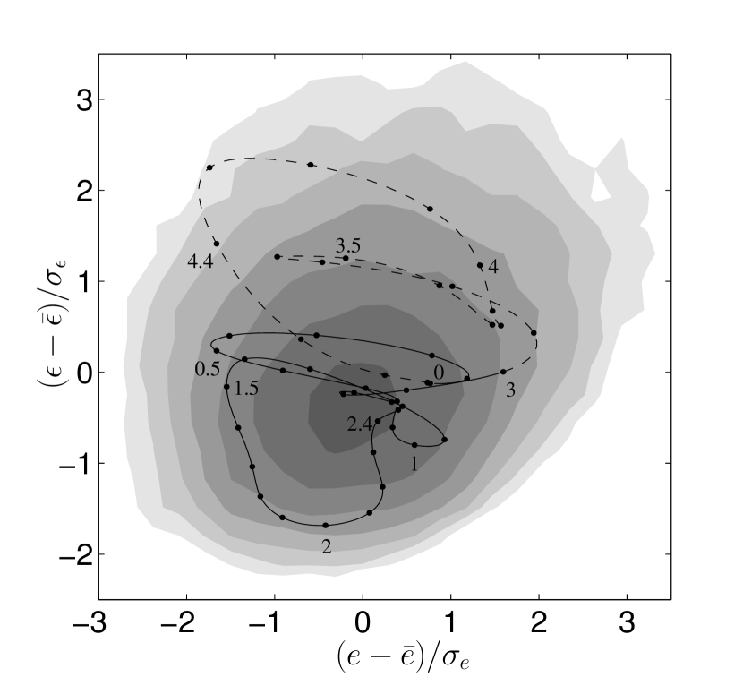
Figure 6: The period-5 orbit and the probability density function of the turbulent state projected on the ($e$, $\epsilon$)-plane at $\nu=0.0035$. The periodic orbit of period $T_{5{\rm p}}=4.91T_{\rm{\scriptscriptstyle R}}$ is represented by a closed curve with solid ($t/T_{\rm{\scriptscriptstyle R}}<3$) and dashed ($t/T_{\rm{\scriptscriptstyle R}}>3$) parts in the low-activity and high-activity periods, respectively. Dots are attached at every $0.1T_{\rm{\scriptscriptstyle R}}$. Numbers indicates the time in the unit of $T_{\rm{\scriptscriptstyle R}}$. Contours of the probability density function are drawn at $80\%$ of its peak value and successive factors of $0.5$ with larger values in darker areas. On the axes the energy input rate and dissipation rate are shown as deviations from their temporal mean normalised by their standard deviation in turbulence.

It is impossible to show how close this orbit is to the turbulent state in the $n$-dimensional phase space, but we can get an impression by looking at its projection on the two-dimensional $(e,\epsilon)$-plane spanned by the energy-input rate and the energy-dissipation rate. In Fig. 6, we plot this projection of the orbit for $\nu=0.0035$ by a closed curve with dots at every $0.1T_{\rm{\scriptscriptstyle R}}$. The solid and dashed parts of the curve respectively indicate the low-activity and high-activity periods described below. Numbers attached to the orbit are measured from an arbitrary reference time near the beginning of the low-activity period and normalised by the return time $T_{\rm{\scriptscriptstyle R}}$. Contours of grey scale show the probability density function of the turbulent state with larger values in darker areas. Both axes are normalised by the standard deviation around the temporal mean of the respective quantitites in turbulence.

This figure has several interesting features. First, the probability density function of turbulent state is slightly skewed towards high $e$ and high $\epsilon$, and the peak is located at the lower-left side of the origin. This is due to bursting events in which anomalous amounts of kinetic energy are injected and dissipated. The periodic orbit makes a large excursion to high-$\epsilon$ corresponding to such a burst Secondly, the distance of the periodic orbit from the origin remains of the order of the standard deviations of turbulence. This is consistent with the picture that this orbit is embedded in the turbulent state. In fact, both the mean values and the standard devations of $e(t)$ and $\epsilon(t)$ are strikingly close for the turbulence and the periodic motion; namely, they are $\overline{e}=\overline{\epsilon}=0.0998$, $\sigma_{e}=0.0352$, $\sigma_{\epsilon}=0.0155$ for the former and $\overline{e}^{5{\rm p}}=\overline{\epsilon}^{5{\rm p}}=0.107$, $\sigma_{e}^{5{\rm p}}=0.0348$, $\sigma_{\epsilon}^{5{\rm p}}=0.0141$ for the latter. The standard deviation of $e(t)$ is larger than that of $\epsilon(t)$ by about factor 2. The magnitude of fluctuations of the present turbulence is about 35% of the mean values in the energy-input rate ($\sigma_{e}/\overline{e}=0.353$), and 16% in the energy-dissipation rate ($\sigma_{\epsilon}/\overline{\epsilon}=0.156$). Thirdly, although the trajectory of the periodic orbit is not simple, we can see that it generally rotates counter-clockwise. In other words, peaks of $\epsilon(t)$ come after those of $e(t)$, which is consistent with the picture of energy cascade to larger wavenumbers (see Fig. 9). Fourthly, the orbit may be divided into two periods. During the first period (solid line) of about $3T_{\rm{\scriptscriptstyle R}}$, $e(t)$ and $\epsilon(t)$ are near or below their mean values. This is the period of low activity. It is followed by a period of high activity (dashed line) of about $2T_{\rm{\scriptscriptstyle R}}$. Thus, the transitions between the low activity and the high activity phase take place on a time scale $T_{\rm{\scriptscriptstyle T}}$, the large-eddy-turnover time. Dots are drawn on the periodic orbit at equal time intevals so that we can get an impression of the speed of the state point along the orbit, which tends to be higher during the high activity phase.

(a)

(b)

Figure 7: Energy characteristics of the period-5 orbit. Temporal variations of (a) energy-input rate $e(t)$ (solid line) and energy-dissipation rate $\epsilon(t)$ (dashed line) and (b) energy $\mathcal{E}(t)$ (solid line) and $\epsilon(t)$ (dashed line), the latter normalised to have the same time mean. The horizontal lines indicate the mean values of the respective quantities. The abscissa is the time normalised by $T_{\rm{\scriptscriptstyle R}}$.

The time series of $e(t)$ and $\epsilon(t)$, shown in Fig. 7(a) is another representation of the periodic orbit. We see that this periodic motion is composed of five enhanced actions of energy input and dissipation every $T_{\rm{\scriptscriptstyle R}}$. The input rate is stronger in amplitude than the dissipation rate. The oscillation phase is anti-correlated between the two. It is clearly seen from the behaviour of $\epsilon(t)$ that the periods of low activity and high activity are the intervals of $t/T_{\rm{\scriptscriptstyle R}}<3$ and $t/T_{\rm{\scriptscriptstyle R}}>3$, respectively. Both $\epsilon(t)$ and $e(t)$ oscillate around lower (or higher) values than their mean values (denoted by the horizontal line) in the former (or latter) interval. In Fig. 7(b) is shown the time series of energy $\mathcal{E}(t)$, the time-derivative of which is equal to the difference $e(t)-\epsilon(t)$. For comparison, the time series of $\epsilon(t)$ is also plotted after shifting and scaling appropriately. It is interesting that the energy and energy-dissipation rate change quite similarly and that the peaks of the former proceed a little those of the latter. Furthermore, comparison with Fig. 7(a) tells us that peaks of $e(t)$ precede those of $\mathcal{E}(t)$. This order of the peaks represents the energy cascade process.

Another convenient projection to capture the structure of the periodic orbit in the phase space is given by taking an arithmetic average of the square of those components of {$\widetilde{\mbox{\boldmath${\omega}$}}(\mbox{\boldmath${k}$})$} that have the same magnitude of wavenumber $|\mbox{\boldmath${k}$}|$. This is nothing but the enstrophy spectrum, identical to the energy spectrum multiplied by the wavenumber squared. Among others, the one-dimensional longitudinal energy spectrum can readily be compared to laboratory experiments. In Fig. 8, we plot the time-averaged energy spectrum of our simulations with open circles for turbulence and with pluses for the period-5 motion. For comparison, also shown are the laboratory data in shear flow at $R_{\lambda}=130$ with solid circles Champagne et al. (1970) and the asymptotic form at the infinite Reynolds number derived theoretically with a solid line Kida and Goto (1997). It is remarkable that the data of the periodic motion and turbulence agree with each other almost perfectly, providing us with another support of closeness in the phase space of this periodic motion and turbulence. The data nicely collapse onto a single curve beyond the energy containing range, which shows that the agreement between the spectra of periodic and turbulent motion is not an artifact of the high symmetry of the present numerical flow.

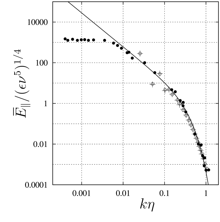
Figure 8: One-dimensional longitudinal energy spectrum. Open circles and pluses represent respectively the turbulent state and the period-5 motion in high-symmetric flow at $R_{\lambda}=67$. Solid circles denote experimental data at $R_{\lambda}=130$ taken from Champagne et al. (1970). The solid line represents the asymptotic form at $R_{\lambda}\rightarrow\infty$ derived theoretical by the sparse direct-interaction approximation Kida and Goto (1997). The axes are normalised according to the Kolmogorov scaling.

So far we have seen that the period-5 motion reproduces the temporal mean energy spectrum of turbulent state remarkably well. A yet more detailed comparison between the period-5 motion and turbulence is provided by the temporal evolution of the energy spectral function. In Fig. 9(a), we show the time series of the three-dimensional energy spectral function calculated as

$$E(k,t)=\frac{1}{2}\sum_{k-\frac{1}{2}\leq|\mbox{\boldmath${\scriptstyle k}$}^{\prime}|<k+\frac{1}{2}}|\widetilde{\mbox{\boldmath${u}$}}(\mbox{\boldmath${k}$}^{\prime},t)|^{2}.$$ (16)

In order to emphasize the fluctuations, the departure from the temporal mean, normalised by the standard deviation of the spectrum, is plotted by contours with positive parts shaded. The abscissa, the wavenumber normalised by the Kolmogorov length, is scaled logarithmically to illuminate the cascade process, thought to be a series of breakdowns of coherent vortical structures into parts about half their size.

It is not straightforward to compare the pattern of $E(k,t)$ of the periodic orbit shown in Fig. 9(a) to that of turbulence because we do not know a priori which parts of a turbulent time sequence are to be compared with. We can, however, select portions of a time series of turbulence that are close to the periodic orbit, as will be explained in the next subsection. In Fig. 9(b), we show such a portion of a time series of $E(k,t)$ of turbulence over the same time interval as the periodic motion. The time variable is the same as in Figs. 6 and 7. The pattern of the energy spectrum of Figs. 9(a) and (b) is remarkably similar, which adds to the evidence that this period-5 orbit represents the turbulent state well. Note especially the inclination and mutual spacing of the streaks which show the cascade process and the relative duration of the

(a)

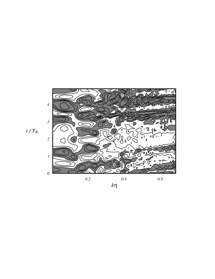
(b)

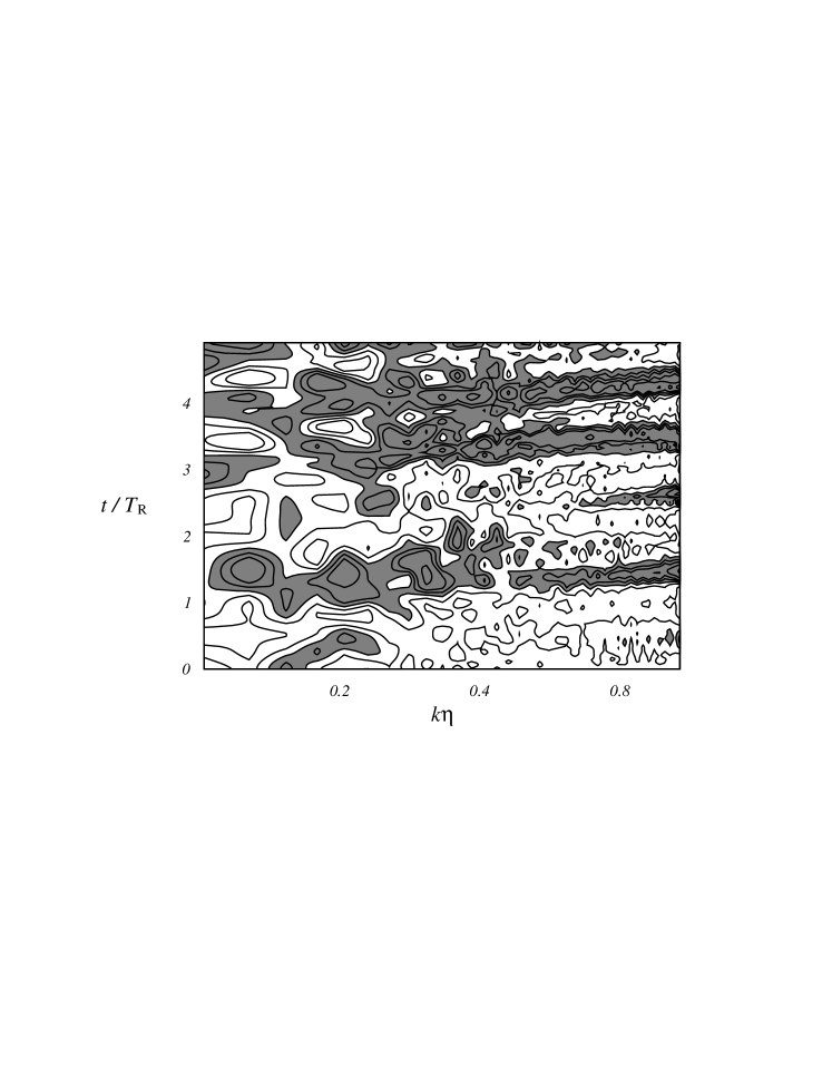
Figure 9: Temporal evolution of energy spectrum. The excess from temporal mean normalised by standard deviation of the three-dimensional energy spectrum $E(k,t)$ is shown by contours at the levels of $0$, $\pm 0.25$, $\pm 0.5$, $\pm 1$, $\pm 2$, the positive parts being shaded. The abscissa is logarithm of the wavenumber normalised by Kolmogorov length $\eta$ and the ordinate is the time normalised by $T_{\rm{\scriptscriptstyle R}}$. (a) period-5 orbit. (b) Fragment from a turbulent time series. The tilted streaks represent anomalies cascading into the dissipation range.

low-activity period ($t/T_{\rm{\scriptscriptstyle R}}<3$) and the high-activity period ($t/T_{\rm{\scriptscriptstyle R}}>3$). Two wide streaks at larger wavenumbers ($k\eta>0.4$) in the later phase of the periodic motion correspond to the excursion to high $\epsilon$ seen in Fig. 6, whereas the other narrow streaks in the earlier phase to the slow excursion. Initial conditions corresponding to other local minima give similar pictures. See Kida and Ohkitani (1992) for a detailed discussion on the energy dynamics at a larger Reynolds number $R_{\lambda}=186$.

5.2 Periodic motion as the skeleton of Turbulence

Motivated by the speculation that the turbulent state approaches the periodic orbit frequently, we introduce a measure of closeness by the ‘distance’ $D(t)$, in the $(e,\epsilon)$ plane, between the periodic orbit and a finite, turbulent time sequence of lenght $T_{\rm{\scriptscriptstyle T}}$ as

$$D(t)^{2}=\frac{1}{2T_{\rm{\scriptscriptstyle T}}}\min_{0\leq t^{*}<T_{5\rm{\scriptscriptstyle p}}}\int_{-\frac{1}{2}T_{\rm{\scriptscriptstyle T}}}^{\frac{1}{2}T_{\rm{\scriptscriptstyle T}}} \Big{[}\frac{1}{\sigma_{\epsilon}^{2}}(\epsilon^{5{\rm p}}(t^{*}+t^{\prime})-\epsilon(t+t^{\prime}))^{2}$$ (17)

$$+\frac{1}{\sigma_{e}^{2}}(e^{5{\rm p}}(t^{*}+t^{\prime})-e(t+t^{\prime}))^{2}\Big{]}\mbox{d}t^{\prime},$$

Figure 10: Temporal variation of the distance $D(t)$ between the turbulent state and the period-5 motion over an arbitrary time interval. The horizontal lines denote the time mean $\overline{D}$ (solid) and $\overline{D}-\sigma_{\rm{\scriptscriptstyle D}}$ (dashed). The abscissa is the time normalised by large-eddy-turnover time $T_{\rm{\scriptscriptstyle T}}$. Observe that the frequency of appearance of sharp minima is of $O(T_{\rm{\scriptscriptstyle T}})$.

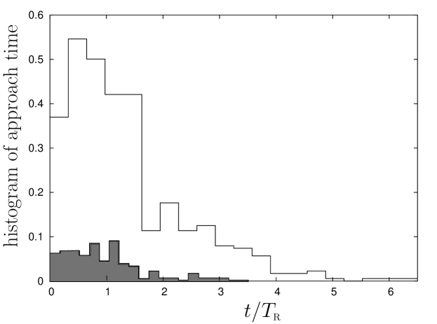
Figure 11: Frequency distribution of approach time of turbulent state to the period-5 motion. The histgrams of time during which $D(t)<\overline{D}-\sigma_{\rm{\scriptscriptstyle D}}$ and $D(t)<\overline{D}-1.5\sigma_{\rm{\scriptscriptstyle D}}$ are shown by white and grey steps, respectively. The area of the former histgram is normalised to unity. The mean values of the approach time are $1.33T_{\rm{\scriptscriptstyle R}}$ ($=0.66T_{\rm{\scriptscriptstyle T}}$) and $0.91T_{\rm{\scriptscriptstyle R}}$ ($=0.45T_{\rm{\scriptscriptstyle T}}$) for the respective cases.

where $\epsilon^{5{\rm p}}(t)$ and $e^{5{\rm p}}(t)$ denote the energy-dissipation rate and energy-input rate along the orbit, respectively. This distance is normalised such that, if wereplace $\epsilon^{5{\rm p}}(t)$ and $e^{5{\rm p}}(t)$ by their respective mean values in the turbulent state, the temporal mean of $D(t)$ is unity. A time series of $D(t)$ taken from a long integration is shown in Fig. 10 together with the temporal mean $\overline{D}$ ($=0.776$) and the temporal mean minus the standard deviation $\overline{D}-\sigma_{\rm{\scriptscriptstyle D}}$ ($=0.535$). It can be seen that $D(t)$ takes sharp minima at the rate of once over the period of $O(T_{\rm{\scriptscriptstyle T}})$, implying that the turbulent state approaches the period-5 orbit at intervals of about one large-eddy-turnover time.

In order to discuss the approach frequency of the turbulent state to the period-5 orbit quantitatively, we consider the statistics of intersections between $D(t)$ and the two horizontal lines. We may say that the turbulent state is located within $\overline{D}$ (or $\overline{D}-\sigma_{\rm{\scriptscriptstyle D}}$) distance from the periodic orbit when $D(t)<\overline{D}$ (or $D(t)<\overline{D}-\sigma_{\rm{\scriptscriptstyle D}}$). The intervals between two consecutive intersection times with $D(t)$ below the holizontal lines are called the approach time, which are regarded as the periods when the turbulent state are close to the periodic orbit. The approach time is different depending on the threshold distance. In Fig. 11, we plot their histgrams, obtained from a time series of about $7,000$ non-normalised time units, for two threshold distances, $\overline{D}-\sigma_{\rm{\scriptscriptstyle D}}$ (white steps) and $\overline{D}-1.5\sigma_{\rm{\scriptscriptstyle D}}$ (grey steps). The area is normalised to be unity for the former histogram. The mean approach times are $1.33T_{\rm{\scriptscriptstyle R}}$ ($0.66T_{\rm{\scriptscriptstyle T}}$) and $0.91T_{\rm{\scriptscriptstyle R}}$ ($0.45T_{\rm{\scriptscriptstyle T}}$) for the respective thresholds, implying that the turbulent state is likely to stay around the period-5 orbit over the time of $\text{O}(T_{\rm{\scriptscriptstyle T}})$ every time it approaches.

How frequently the turbulent state approaches the periodic orbit may be measured by the time intervals between consecutive approach periods, which is called the approach interval. Note that this measure is more appropriate than counting the local minimum times of $D(t)$ in Fig. 10 because two or more minima may occur in one approach interval. In Fig. 12, we plot the histgrams of the approach interval made by using the same data as that for Fig. 11. Again, the white and grey steps indicate the histgrams for the threshold distances of $\overline{D}-\sigma_{\rm{\scriptscriptstyle D}}$ and $\overline{D}-1.5\sigma_{\rm{\scriptscriptstyle D}}$, respectively. The area is normalised to be unity for the former one. The mean approach intervals are $5.8T_{\rm{\scriptscriptstyle R}}$ ($=2.9T_{\rm{\scriptscriptstyle T}}$) and $28.0T_{\rm{\scriptscriptstyle R}}$ ($=14.0T_{\rm{\scriptscriptstyle T}}$) for the respective thresholds. This result tells us that the turbulent state approaches the period-5 orbit at the rate of once over a few eddy-turnover times (or about the period of this periodic orbit) within distance of $\overline{D}-\sigma_{\rm{\scriptscriptstyle D}}$ and that a more closer approach within distance of $\overline{D}-1.5\sigma_{\rm{\scriptscriptstyle D}}$ is observed much less frequently, i.e. once over $14$ eddy-turnover times.

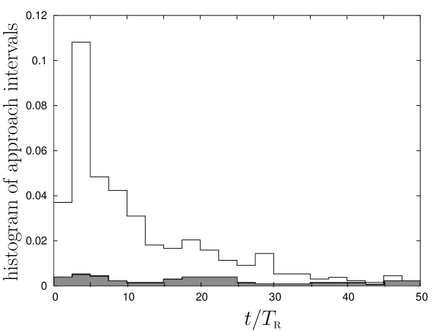
Figure 12: Frequency distribution of approach intervals of turbulent state to the period-5 motion. The histgrams of time interval between midpoints of segments with $\overline{D}-\sigma_{\rm{\scriptscriptstyle D}}$ and $\overline{D}-1.5\sigma_{\rm{\scriptscriptstyle D}}$ are shown by white and grey steps, respectively. The area of the former histgram is normalised to unity. The mean values of the interval is $5.8T_{\rm{\scriptscriptstyle R}}$ ($=2.9T_{\rm{\scriptscriptstyle T}}$) and $28.0T_{\rm{\scriptscriptstyle R}}$ ($=14.0T_{\rm{\scriptscriptstyle T}}$) for the respective segments.

Which parts of the periodic orbit is the turbulent state likely to approach more frequently ? This information is provided by the phase time $t^{*}$ that defines the distance $D(t)$, i.e. that gives the minimum value of the integration in (17). In Fig. 13, we show the histgrams of the phase time of approach of turbulent state for threshold distances of $\overline{D}-\sigma_{\rm{\scriptscriptstyle D}}$ (white steps) and $\overline{D}-1.5\sigma_{\rm{\scriptscriptstyle D}}$ (grey steps). The area is normalised to be unity for the former histgram. For comparison, the PDF of realisation of the turbulent state along the period-5 orbit is drawn with a dotted curve. This density is obtained by integrating the PDF shown in Fig. 6 over a small neigbourhood (a disk with a radius much smaller than the standard deviations $\sigma_{e}$ and $\sigma_{\epsilon}$) of a given point on the period-5 orbit and multiplying by the local speed of the state point. It is interesting that the approach phase is localised in the low-active period ($t^{*}/T_{\rm{\scriptscriptstyle R}}<3$), but hardly observed in the high-active period ($t^{*}/T_{\rm{\scriptscriptstyle R}}>3$). This tendency of non-uniform appoach suggests that the movement of the state point of turbulence may be more violent in the high-active period than in the low-active period. The stability characteristics, in the phase space, of the state point will be examined by the local Lyapunov analysis in the next subsection. Incidentally, the totally different behaviour between the histgrams (steps) of the approach phase and the existing probability (dotted curve) of turbulent state indicates that the non-uniformity of the approach phase may be due to that of the dynamical properties along the periodic orbit.

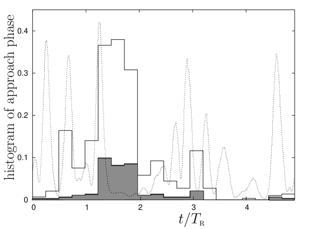
Figure 13: Frequency distribution of the phase of the period-5 motion at which the turbulent state approaches. The histgrams of the phase at the mid-point of segments with $D(t)<\overline{D}-\sigma_{\rm{\scriptscriptstyle D}}$ and $D(t)<\overline{D}-1.5\sigma_{\rm{\scriptscriptstyle D}}$ are shown by white and grey steps, respectively. The area of the former histgram is normalised to unity. The dotted curve indicates the existing probability of the turbulent state on the period-5 orbit projected on the $(e,\epsilon)$-plane.

In order to get an idea of what the turbulent orbit looks like when it is approaching the period-5 motion, we show in Fig. 14 such segments of length $T_{\rm{\scriptscriptstyle T}}$ that satisfy $D(t)<\overline{D}-1.5\sigma_{\rm{\scriptscriptstyle D}}$ in the $(e,\epsilon)$ plane which are selected arbitrarily from a long turbulent orbit. Observe the way that the turbulent state is attracted around the period-5 motion quite well, though such beautiful examples are not so frequent, i.e. only at the rate of once every $24T_{\rm{\scriptscriptstyle T}}$.

Figure 14: Turbulent orbits close to the period-5 motion. Such segments of length $T_{\rm{\scriptscriptstyle T}}$ that satisfy $D(t)<\overline{D}-1.5\sigma_{\rm{\scriptscriptstyle D}}$ in the $(e,\epsilon)$ plane are selected arbitrarily from a long turbulent orbit, and four examples are drawn in the respective figures. The dotted closed line indicates the priod-5 orbit.

5.3 Lyapunov characteristics

Lyapunov exponents describe the growth or decay of perturbations with respect to a given reference solution of a dynamical system. The Lyapunov exponents are a benchmark of chaos theory. If at least one exponent is positive, corresponding to a growing perturbation, the system is chaotic and there is sensitive dependence on initial conditions and a strange attractor with a fractal dimension. The rate at which information about the initial condition is lost and the dimension of the chaotic attractor can be computed from the Lyapunov exponents. Although turbulence can be regarded as a form of high dimensional chaos, its Lyapunov characteristics are far from understood. Here, we will investigate the Lyapunov characteristics of isotropic turbulence by means of the embedded periodic solution.

The Navier-Stokes equation (3) can be written symbolically as

$$\frac{\rm d}{{\rm d}t}{\mbox{\boldmath${x}$}}=\mbox{\boldmath${f}$}(\mbox{\boldmath${x}$},\nu),$$ (18)

where $\mbox{\boldmath${x}$}\in\mathbb{R}^{n}$ is a vector that holds the Fourier transform of the vorticity, $\widetilde{\mbox{\boldmath${\omega}$}}$, and ${f}$ denotes the right-hand side of Eq. (3). The linearised equations are then given by

$$\frac{\rm d}{{\rm d}t}{\mbox{\boldmath${v}$}}=\mbox{\boldmath${J}$}\mbox{\boldmath${v}$},$$ (19)

where ${v}$ denotes a perturbation vorticity field $\delta\widetilde{\mbox{\boldmath${\omega}$}}$, and ${J}$ is the Jacobian matrix, i.e. $J_{ij}=\partial f_{i}(\mbox{\boldmath${x}$}(t),\nu)/\partial x_{j}$. The average rate of growth or decay of a perturbation is measured by the Lyapunov exponent

$$\mathchar 28931\relax=\lim_{t\rightarrow\infty}\frac{1}{2t}\ln\frac{\|\mbox{\boldmath${v}$}(t)\|_{\rm{\scriptscriptstyle{Q}}}}{\|\mbox{\boldmath${v}$}(0)\|_{\rm{\scriptscriptstyle{Q}}}},$$ (20)

where $\|\cdot\|_{\rm{\scriptscriptstyle{Q}}}$ again denotes the enstrophy norm and a factor of $1/2$ is included because this norm is quadratic.

In general, the value of $\mathchar 28931\relax$ depends on the reference solution $\mbox{\boldmath${x}$}(t)$ and on the initial perturbation $\mbox{\boldmath${v}$}(0)$. However, in systems with a chaotic attractor the Oseledec theorem guarantees that there is a spectrum of limit values, $\{\mathchar 28931\relax_{i}\}_{i=1}^{n}$, unique for the attractor. At almost every initial point $\mbox{\boldmath${x}$}(0)$ there are $n$ initial perturbations $\mbox{\boldmath${v}$}_{i}(0)$ such that $\mathchar 28931\relax_{i}=\lim_{t\rightarrow\infty}(1/2t)\ln\left(\|\mbox{\boldmath${v}$}_{i}(t)\|_{\rm{\scriptscriptstyle{Q}}}/\|\mbox{\boldmath${v}$}_{i}(0)\|_{\rm{\scriptscriptstyle{Q}}}\right)$. The vectors $\mbox{\boldmath${v}$}_{i}(t)$ are called the Lyapunov vectors and depend on the initial point in a complicated manner. The Oseledec theorem holds for almost every initial point in the basin of attraction of the chaotic attractor in a measure theoretic sense. This means that starting from any generic initial condition we will find the same Lyapunov spectrum, but for certain special initial points the spectrum may differ. Examples of such special initial points are points lying on periodic solutions.

The Lyapunov spectrum of chaotic motion can be used to measure the ‘strength’ of the chaos or the complexity of the motion. Suppose that the Lyapunov exponents are ordered such that $\mathchar 28931\relax_{1}>\mathchar 28931\relax_{2}>\ldots>\mathchar 28931\relax_{n}$, then the Kolmogorov-Sinai entropy is defined by

$$H_{\rm{\scriptscriptstyle KS}}=\sum_{i=1}^{k}\mathchar 28931\relax_{i},\qquad\text{where}\ \ \mathchar 28931\relax_{k}>0\ \text{and}\ \ \mathchar 28931\relax_{k+1}<0,$$ (21)

i.e. the sum of positive Lyapunov exponents, and the Kaplan-Yorke dimension is defined by

$$D_{\rm{\scriptscriptstyle KY}}=k+\frac{1}{|\mathchar 28931\relax_{k+1}|}\sum_{i=1}^{k}\mathchar 28931\relax_{i},\qquad\text{where}\ \ \sum_{i=1}^{k}\mathchar 28931\relax_{i}>0\ \text{and}\ \ \sum_{i=1}^{k+1}\mathchar 28931\relax_{i}<0.$$ (22)

One way to interpret these definitions is to realise that a volume element contained in the subspace spanned by any number of Lyapunov vectors will grow or decay at a rate given by the sum of the corresponding Lyapunov exponents. Thus, the Kolmogorov-Sinai entropy is the maximal rate of expansion for any volume element. It quantifies the unpredictability of the dynamics. The Kaplan-Yorke dimension can be thought of as the dimension of the chaotic attractor. Its integer part is the dimension of the largest volume element that will grow in time, and the fractional part is added to render the function continuous in the Lyapunov exponents.

The numerical computation of more than only the leading Lyapunov exponent is troublesome in systems with many degrees of freedom. The algorithms at hand require simultaneous integration of several perturbation vectors and the repeated application of Gramm-Schmidt orthogonalisation (see e.g. Wolf et al. (1985)). This introduces numerical error, especially when applied to truncations of the Navier-Stokes equation with small amplitude fluctuations in the large wavenumber components. The limit in Eq.(20) has to be replaced by an average over a finite time interval of the growth rate, and the convergence of $\mathchar 28931\relax$ with time can be rather slow, of order $\mbox{O}(1/\sqrt{t})$. Consequently, early attempts to compute a part of the Lyapunov spectrum for turbulent flows were restricted to simulations at low resolution. Results for isotropic turbulence Grappin and Léorat (1991) and shear turbulence Keefe et al. (1992) indicate that the Kaplan-Yorke dimension is at least of order $\mbox{O}(100)$ even at low Reynolds number.

In simulations at high resolution, the computation of a few hundred Lyapunov exponents is hard if not impossible. One way around this problem is to inspect the local rather than the time average growth rates. The local Lyapunov exponent can be defined by

$$\lambda(t)=\frac{1}{2}\frac{\mbox{d}}{\mbox{d}t}\ln\|\mbox{\boldmath${v}$}(t)\|_{\rm{\scriptscriptstyle{Q}}},$$ (23)

such that, taking the time average, we have $\overline{\lambda}=\mathchar 28931\relax$. The evolution of the Lyapunov vectors and the associated local Lyapunov exponents was studied in the case of weakly turbulent Taylor-Couette flow by Vastano and Moser (1991). They managed to tie the local Lyapunov exponents and vectors to physical instabilities in the transition to chaotic behaviour.

In the same spirit we seek to investigate the Lyapunov characteristics of developed isotropic turbulence. For this purpose we use the period-5 orbit as the reference solution. The choice of a periodic reference solution greatly facilitates the analysis. Let $\mbox{\boldmath${x}$}(t)$ be a solution of Eq.(18) such that $\mbox{\boldmath${x}$}(t+T)=\mbox{\boldmath${x}$}(t)$ for all $t$ and some period $T$. By Floquet theory the solution of Eq.(19) can then be written as

$$\mbox{\boldmath${v}$}(t)=\mbox{\boldmath${M}$}(t)\mbox{e}^{\mbox{\boldmath${\scriptstyle A}$}t}\mbox{\boldmath${v}$}(0),$$ (24)

where $\mbox{\boldmath${M}$}(t)=\mbox{\boldmath${M}$}(t+T)$ is a periodic matrix satisfying $\mbox{\boldmath${M}$}(0)=\mathbb{I}$ (unit matrix), and ${A}$ is a constant matrix. Thus we find that the Lyapunov spectrum $\{\mathchar 28931\relax_{i},\mbox{\boldmath${v}$}_{i}(t)\}$ is determined by the eigenspectrum $\{\mu_{i},\mbox{\boldmath${w}$}_{i}\}$ of ${A}$. For each real eigenvalue $\mu_{i}$ we have $\mathchar 28931\relax_{i}=\mu_{i}$, $\mbox{\boldmath${v}$}_{i}(0)=\mbox{\boldmath${w}$}_{i}$, and for the local exponent we find

$$\lambda_{i}(t)=\mathchar 28931\relax_{i}+\frac{1}{2}\frac{\mbox{d}}{\mbox{d}t}\ln\|\mbox{\boldmath${M}$}(t)\mbox{\boldmath${v}$}_{i}(0)\|_{\rm{\scriptscriptstyle{Q}}}.$$ (25)

For each complex pair $\{\mu_{i},\mu_{i+1}\}$ we have $\mathchar 28931\relax_{i}=\mathchar 28931\relax_{i+1}=\text{Re}\left(\mu_{i}\right)$, $\mbox{\boldmath${v}$}_{i}(0)=\text{Re}\left(\mbox{\boldmath${w}$}_{i}\right)$, $\mbox{\boldmath${v}$}_{i+1}(0)=\text{Im}\left(\mbox{\boldmath${w}$}_{i}\right)$ and

$$\lambda_{i}(t)=\lambda_{i+1}(t)=\mathchar 28931\relax_{i}+\frac{1}{2}\frac{\mbox{d}}{\mbox{d}t}\ln\left(\|\mbox{\boldmath${M}$}(t)\mbox{\boldmath${v}$}_{i}(0)\|_{\rm{\scriptscriptstyle{Q}}}+\|\mbox{\boldmath${M}$}(t)\mbox{\boldmath${v}$}_{i+1}(0)\|_{\rm{\scriptscriptstyle{Q}}}\right).$$ (26)

The matrix $\mbox{e}^{\mbox{\boldmath${\scriptstyle A}$}T}$ is computed in much the same way as we computed the matrix of derivatives of the Poincaré map as described in section 4. We then solve the eigenvalue problem to find any number of Lyapunov exponents and vectors. In order to find the $\lambda_{i}(t)$ we integrate the linearised Navier-Stokes equations along the period-5 orbit with the eigenvectors $\mbox{\boldmath${v}$}_{i}(0)$ as initial condition. In this integration numerical errors in $\mbox{\boldmath${v}$}_{i}(t)$ tend to grow as $\exp([\mathchar 28931\relax_{1}-\mathchar 28931\relax_{i}]t)$, which puts a limit to the number of local Lyapunov exponents we can compute. The results presented below are based on analysis of the first $50$ exponents. The largest and smallest average exponents are $\mathchar 28931\relax_{1}=0.238$ and $\mathchar 28931\relax_{50}=-0.584$.

Figure 15: The largest Lyapunov exponent $\mathchar 28931\relax_{1}$ measured along the periodic orbits, labeled as in figure 5. The value found for turbulent motion is represented by the dotted line.

As mentioned above, the Lyapunov spectrum of periodic motion is different from that of turbulent motion. However, as argued in the preceding subsections we consider the periodic motion as the skeleton of turbulence, and its qualitative properties as an approximation of the corresponding properties of turbulence. Thus the Lyapunov characteristics of the periodic motion are expected to be close to those of turbulence. A direct comparison is given by the leading Lyapunov exponent, which can be computed for the turbulent motion as described in Kida and Ohkitani (1992). Fig. 15 shows $\mathchar 28931\relax_{1}$ for the turbulent motion and for the five periodic orbits in the parameter range $0.0035<\nu<0.004$. As we saw when comparing the energy-dissipation rate of periodic and turbulent motion in Fig. 5, the period-5 orbit reproduces the values found for turbulent motion well, whereas the shorter periodic orbits deviate. At the time of writing, the continuation curves for the period-3 and period-4 orbits were incomplete. Further computations are in progress. The numerical values at $\nu=0.0035$ are $\mathchar 28931\relax_{1}=0.2$ and $\mathchar 28931\relax_{1}^{5\rm{p}}=0.238$ for the turbulent and the period-5 motion, respectively.

As we know only the leading Lyapunov exponent for turbulent flow, we cannot directly estimate $H_{\rm{\scriptscriptstyle KS}}$ and $D_{\rm{\scriptscriptstyle KY}}$ for the chaotic attractor. For the period-5 motion we find that $H_{\rm{\scriptscriptstyle KS}}^{5\rm{p}}=0.992$ and $D_{\rm{\scriptscriptstyle KY}}^{5\rm{p}}=19.7$. Note, that these values cannot directly be compared to those for general isotropic turbulence because we can only compute the contribution of perturbations that satisfy the high-symmetry constraints described in section 2. In the full phase space, without any symmetry constraints, these values are likely to be a factor of order $\mbox{O}(100)$ times higher. The local Kolmogorov-Sinai entropy $h_{\rm{\scriptscriptstyle KS}}(t)$ and local Kaplan-Yorke dimension $d_{\rm{\scriptscriptstyle KY}}(t)$ can be computed from the local Lyapunov exponents, substituting the $\lambda_{i}(t)$ for the $\mathchar 28931\relax_{i}$ in Eqs. (21) and (22). Thus, we get an impression of the change of the complexity of the flow with time. The graph is shown in Fig. 16. Note that, strictly speaking, we can only compute a lower bound for the local quantities as we only know the leading 50 local Lyapunov exponents. However, $\lambda_{50}(t)$ is negative at all times and we expect only minor contributions, if any, from higher exponents.

Figure 16: The local Kaplan-Yorke dimension $d_{\rm{\scriptscriptstyle KY}}(t)$ (solid line) and the local Kolmogorov-Sinai entropy $h_{\rm{\scriptscriptstyle KS}}(t)$ (nondimensionalised by $T_{\rm{\scriptscriptstyle T}}$ and drawn with a dotted line) as computed from the leading 50 local Lyapunov exponents $\{\lambda_{i}(t)\}_{i=1}^{50}$ along the period-5 orbit. Note the rapid oscillations and large amplitude.

The local Lyapunov exponents and the derived quantities $h_{\rm{\scriptscriptstyle KS}}(t)$ and $d_{\rm{\scriptscriptstyle KY}}(t)$ show large fluctuations on a time scale as short as the Kolmogorov dissipation time scale $\tau_{\eta}=\sqrt{\nu/\bar{\epsilon}}\approx 0.2$. Around $t/T_{\rm{\scriptscriptstyle R}}=4$ in the active phase identified in section 5.1, $d_{\rm{\scriptscriptstyle KY}}(t)$ jumps from $0$ to a wide maximum larger than $50$ and back. This peak coincides with the dominant peak of the energy-dissipation rate. The second wide maximum lies around $t/T_{\rm{\scriptscriptstyle R}}=4.9$ and coincides with a peak of the energy-input rate. Thus it seems that the local Lyapunov exponents and the complexity of the flow are correlated to physical, spatial mean quantities.

Figure 17: Coefficient of correlation of the local Lyapunov exponents $\lambda_{i}(t)$ with the energy-input rate (filled circles) and the energy-dissipation rate (open circles). Despite a fair amount of scatter we can see that the exponents $\lambda_{i}(t)$ with $1\leq i<D_{\rm{\scriptscriptstyle KY}}$ behave differently from those of higher indices.

In order to check this conjecture we compute the correlation between the $\lambda_{i}(t)$ on one hand, and $e(t)$ and $\epsilon(t)$ on the other. The correlation coefficients are defined by

$$c^{i}_{e}=\frac{1}{T_{5\rm{p}}\sigma_{e}^{5\rm{p}}\sigma_{\lambda_{i}}}\int_{0}^{T_{5\rm{p}}}(e^{5\rm{p}}(t)-\bar{e}^{5\rm{p}})(\lambda_{i}(t)-\mathchar 28931\relax_{i})\mbox{d}t,$$

$$c^{i}_{\epsilon}=\frac{1}{T_{5\rm{p}}\sigma_{\epsilon}^{5\rm{p}}\sigma_{\lambda_{i}}}\int_{0}^{T_{5\rm{p}}}(\epsilon^{5\rm{p}}(t)-\bar{\epsilon}^{5\rm{p}})(\lambda_{i}(t)-\mathchar 28931\relax_{i})\mbox{d}t,$$ (27)

where $\sigma_{\lambda_{i}}$ is the standard deviation of $\lambda_{i}(t)$. Fig. 17 shows $c^{i}_{e}$ and $c^{i}_{\epsilon}$ for the first 50 local Lyapunov exponents. Although there is a lot of scatter in the data, a structural difference between the local Lyapunov exponents with a small and a large index is obvious. Those with a small index have a negative correlation with the energy-dissipation rate and a positive correlation with the energy-input rate, whereas those with a large index have a positive correlation with the energy-dissipation rate and a correlation of either sign with the energy-input rate. This suggests that the Lyapunov vectors have a preferred spatial scale. In particular, we conjecture that the Lyapunov vectors with a small index describe perturbation fields with a large spatial scale, directly excited by the energy input. Those with a larger index describe smaller scale perturbation fields and are more strongly correlated to energy dissipation.

(a)

(b)

Figure 18: Temporal variation of (a) $\widetilde{\lambda}_{\rm{\scriptscriptstyle I}}(t)$ and (b) $\widetilde{\lambda}_{\rm{\scriptscriptstyle II}}(t)$. The running average is taken over $\tau_{\rm{av}}=0.54T_{\rm{\scriptscriptstyle R}}$. For comparison the energy-input and dissipation rates, shifted and scale by equal amounts, are drawn with a dotted and a dashed line, respectively. The horizontal lines indicate the time mean values, $\overline{\lambda}_{\rm{\scriptscriptstyle I}}=0.122$ and $\overline{\lambda}_{\rm{\scriptscriptstyle II}}=-5.57$.

In order to test this conjecture we divide the Lyapunov spectrum into two parts with an equal number of exponents. As indicated in Fig. 17, we choose the integer part of the Kaplan-Yorke dimension, computed from the time averaged Lyapunov exponents, to separate the two. Thus, group I comprises $\{\mathchar 28931\relax_{i},\mbox{\boldmath${v}$}_{i}\}_{i=1}^{19}$ and group II comprises $\{\mathchar 28931\relax_{i},\mbox{\boldmath${v}$}_{i}\}_{i=20}^{38}$. The growth rate of volumes in these two subspaces is given by $\lambda_{\rm{\scriptscriptstyle I}}(t)=\sum_{i=1}^{19}\lambda_{i}(t)$ and $\lambda_{\rm{\scriptscriptstyle II}}(t)=\sum_{i=20}^{38}\lambda_{i}(t)$, respectively. As mentioned above, the $\lambda_{i}(t)$ fluctuates rapidly. In order to see a possible correlation with the energy-input and dissipation rates we compute the running mean of $\lambda_{\rm{\scriptscriptstyle I}}(t)$ and $\lambda_{\rm{\scriptscriptstyle II}}(t)$ over a time interval $\tau_{\rm{av}}$ such that $\tau_{\eta}<\tau_{\rm{av}}<T_{\rm{\scriptscriptstyle R}}$. The running mean is indicated by a tilde. Figs. 18(a) and (b) show the time series of $\widetilde{\lambda}_{\rm{\scriptscriptstyle I}}(t)$ and $\widetilde{\lambda}_{\rm{\scriptscriptstyle II}}(t)$ along with the energy-input and dissipation rates, shifted to have the same time mean value and scaled by equal factors. Clearly, $\widetilde{\lambda}_{\rm{\scriptscriptstyle I}}(t)$ has a strong positive correlation with the energy-input rate and a weaker, negative correlation with the energy-dissipation rate. Most of the peaks of $\widetilde{\lambda}_{\rm{\scriptscriptstyle I}}(t)$ coincide with peaks of the energy-input rate, the latter leading in phase. Only in the interval $2<t/T_{\rm{\scriptscriptstyle R}}<3$ the correlation is not very clear. In contrast, $\widetilde{\lambda}_{\rm{\scriptscriptstyle II}}(t)$ shows a strong positive correlation with the energy-dissipation rate and tends to lead in phase. On the interval $0<t/T_{\rm{\scriptscriptstyle R}}<1$ the correlation with the energy-dissipation rate is weaker, and locally there is a positive correlation with the energy-input rate.

Finally we consider the orientation of the Lyapunov vectors. Consider the Lyapunov vectors scaled to unit length, $\hat{\mbox{\boldmath${v}$}}_{i}=\mbox{\boldmath${v}$}_{i}(t)/\|\mbox{\boldmath${v}$}_{i}(t)\|_{\rm{\scriptscriptstyle{Q}}}^{1/2}$ and denote the corresponding perturbation vorticity field by $\delta\hat{\widetilde{\mbox{\boldmath${\omega}$}}}_{i}$. We compute the enstrophy spectrum of the scaled perturbation fields as

$$Q_{i}(k)=\frac{1}{2}\sum_{k-\frac{1}{2}<\|\mbox{\boldmath${k}$}\|<k+\frac{1}{2}}|\delta\hat{\widetilde{\mbox{\boldmath${\omega}$}}}_{i}(\mbox{\boldmath${k}$})|^{2}.$$ (28)

If the Lyapunov vectors have a preferred length scale we expect to see a structural difference between the enstrophy spectra of the vectors in group I and group II, the former having a larger amplitude in the smaller wavenumbers and the latter in the larger wavenumbers. In Fig. 19, we plot the average spectrum over the perturbation fields in group I, $Q_{\rm{\scriptscriptstyle I}}(k)$, and group II, $Q_{\rm{\scriptscriptstyle II}}(k)$. All perturbation fields have the maximal amplitude around $k\eta=0.4$, corresponding to a spatial scale in between that of the fixed modes, $k_{f}^{-1}$, and the Kolmogorov dissipation scale $\eta$ in the current simulations. The average spectrum $Q_{\rm{\scriptscriptstyle I}}(k)$ is larger for all wavenumbers below $k_{\rm{c}}$ ($\approx 0.32$) and smaller for most larger wavenumbers.

These results indicate that the Lyapunov vectors indeed have preferred length scales associated with them, and that the local Lyapunov exponents are correlated with the physical quantities that dominate these spatial scales. We have checked that the results do not depend critically on the choice of the two groups, i.e. the highest index in group I, here fixed to the integer part of the Kaplan-Yorke dimension $D_{\rm{\scriptscriptstyle KY}}$. As far as we know, this is the first time that evidence is found for the localisation of Lyapunov vectors and the correlation of (local) Lyapunov exponents and physical quantities in developed turbulence. The localisation of Lyapunov vectors has been found in shell model turbulence by Yamada and Ohkitani (1998) (and references therein). However, their results are derived at much larger Reynolds number, in the presence of a large inertial range. We expect that the presence of a developed inertial range in the case of isotropic turbulence would yield an even clearer separation of spatial scales than seen in our present results.

Figure 19: Enstrophy spectra $Q_{\rm{\scriptscriptstyle I}}(k)$ and $Q_{\rm{\scriptscriptstyle II}}(k)$ of the perturbation vorticity fields $\delta\hat{\mbox{\boldmath${\omega}$}}_{i}$ in the groups I and II. The filled circles represent the average profile of Lyapunov vectors 1 through 19, the open circles represent the average profile of Lyapunov vectors 20 through 38. The average profile of the leading 19 Lyapunov vectors is larger for $k\eta<k_{\rm{c}}\eta\approx 0.32$ and mostly smaller for larger wave numbers.

6 Concluding Remarks

We have identified temporally periodic motion which reproduces the dynamics and statistics of isotropic turbulence well in high-symmetric flow. The period of the periodic motion is of the order of the eddy-turnover time of turbulence. The mean properties of various physical quantities, e.g. the energy spectral function and the Lyapunov exponent, calculated by time average taken over one period of the periodic motion approximate those of the turbulence taken over a long time series. This agreement may be understood by noting the fact that the turbulent motion spends much of the time in the same, or similar, spatio-temporal state as the periodic motion. In fact, we have seen that the state point of the turbulent motion approaches the orbit of the periodic motion in phase space at the rate of once over several eddy-turnover times. In other words, the orbit of this periodic motion is embedded in turbulence. Thus, we regard it as the skeleton of turbulence.

Such a periodic motion embedded in turbulence is useful as a reference field with respect to which the mechanisms of various turbulence phenomena, including turbulent mixing and the energy-cascade process, can be analysed. The reason is as follows. Turbulence is intrinsically chaotic and the fluid flow varies quite randomly both in space and in time. The fluid motion is unpredictable and never repeats, though the statistical properties are rather universal. This chaotic nature makes it difficult to study the general properties of turbulence. There is no way to confirm that those turbulence data used in analysis represent typical properties of turbulence. On the other hand, the periodic motion, whose dynamical properties can be understood much more clearly than those of the turbulence itself, repeats exactly its temporal variation without limit. Then, by analysing the repeated, periodic time series we may be able to extract the typical mechanisms of turbulence dynamics as well as calculate the statistics of any physical quantities with high accuracy. This line of study is now under way.

In the present study the inertial range is captured only marginally. In order to increase the resolution it is necessary to simulate high-Reynolds number turbulence. The difficulties then arise in the computation time and memory requirements of the algorithm used to find periodic motion. The calculation of iteration matrix of the Newton-Raphson procedure is most time-consuming. The number of degrees of freedom in our computations, $\rm{O}(10^{4})$, seems to be the maximal number tackled in continuation of periodic orbits at the time of writing. It proved possible to use the conventional arc-length method with the Newton-Raphson iteration because of the high efficiency of parallelization. In order to go to higher truncation levels, and thus larger Reynolds numbers and a developed inertial range, it may be necessary to switch to matrix-free methods for continuation. Such methods use inexact linear solvers for equations like (14), avoiding the computation and orthogonal decomposition of the matrix of derivatives. Recently this approach has successfully been applied to the computation of periodic solutions of the Navier-Stokes equations Sánchez et al. (2004).

It is conjectured that there are infinitely many periodic orbits in the turbulent regime. Some of them represent turbulent state and the others do not. From the present study we cannot infer a general rule for selecting periodic motion which represents the turbulence well. It is interesting to see, that at low micro-scale Reynolds number, where we distill the periodic orbits from a turbulent time series, their time mean energy-dissipation rate and largest Lyapunov exonent are all close to those of turbulence. If we decrease the viscosity, however, only the orbit of longest period reproduces the average values of turbulence. Future work should aim at a better understanding of this selection process as well as of the uniqueness of such solutions.

References

- Artuso et al. (1990) Artuso, R., Aurell, E. and Cvitanović, P. 1990 Recycling of strange sets: I. Cycle expansions. Nonlinearity 3, 325–359.
- Boratav and Pelz (1997) Boratav, O.N. and Pelz, B.P. 1997 Structures and structure functions in the inertial range of turbulence. Phys. Fluids 9, 1400–1415.
- Champagne et al. (1970) Champagne, F.H., Harris, V.G. and Corrsin, S. 1970 Experiments on nearly homogeneous turbulent shear flow. J. Fluid. Mech. 41, 81–139.
- Christiansen et al. (1997) Christiansen, F., Cvitanović, P. and Putkaradze, V. 1997 Spatiotemporal chaos in terms of unstable recurrent patterns. Nonlinearity 10, 55–70.
- Grappin and Léorat (1991) Grappin, R. and Léorat, J. 1991 Lyapunov exponents and the dimension periodic incompressible Navier-Stokes flows: numerical measurements. J. Fluid Mech. 222, 61–94.
- Kawahara and Kida (2001) Kawahara, G. and Kida, S. 2001 Periodic motion embedded in plane Couette turbulence: regeneration cycle and burst. J. Fluid Mech. 449, 291–300.
- Kato and Yamada (2003) Kato, S. and Yamada, M. 2003 Unstable periodic solutions embedded in a shell model turbulence. Phys. Rev. E 68, 025302-1–4.
- Keefe et al. (1992) Keefe, L., Moin, P. and Kim, J. 1992 The dimension of attractors underlying periodic turbulent Poiseuille flow. J.Fluid Mech. 242, 1–29.
- Kida (1985) Kida, S. 1985 Three-dimensional periodic flows with high-symmetry. J. Phys. Soc. Japan 54, 2132–2136.
- Kida and Goto (1997) Kida, S. and Goto, S. 1997 A Lagrangian direct-interaction approximation for homogeneous isotropic turbulence. J. Fluid Mech. 345, 307–345.
- Kida and Murakami (1987) Kida, S. and Murakami, Y. 1987 Kolmogorov similarity in freely decaying turbulence. Phys. Fluids 30, 2030–2039.
- Kida and Murakami (1989) Kida, S. and Murakami, Y. 1989 Statistics of velocity gradients in turbulence at moderate Reynolds number. Fluid Dyn. Res. 4, 347–370.
- Kida et al. (1989) Kida, S., Yamada, M. and Ohkitani, K. 1989 A route to chaos and turbulence. Physica D 37, 116–125.
- Kida and Ohkitani (1992) Kida, S. and Ohkitani, K. 1992 Spatiotemporal intermittency and instability of a forced turbulence. Phys. Fluids 4, 1018–1027.
- Monin and Yaglom (1975) Monin, A.S. and Yaglom, A.M. 1975. Statistical fluid mechanics: Mechanics of turbulence. Vol. 2, MIT Press.
- Sánchez et al. (2004) Sánchez, J., Net, M., García-Archilla, B. and Simó, C. 2004 Newton-Krylov continuation of periodic orbits for Navier-Stokes flows. J.Comput.Phys. 201, 13–33.
- Schlichting (1979) Schlichting, H. 1979. Boundary-layer theory. Mcagraw-Hill, New York.
- Vastano and Moser (1991) Vastano, J. A. and Moser, R. D. 1991 Short-time Lyapunov exponent analysis and the transition to chaos in Taylor-Couette flow. J. Fluid Mech. 233, 83–118.
- van Veen (2004) van Veen, L. 2004 The quasi-periodic doubling cascade in the transition to weak turbulence. Physica D to appear.
- Wolf et al. (1985) Wolf, A., Swift J.B., Swinney, H.L. and Vastano, J.A. 1985 Determining Lyapunov exponents from a time series. Phys. D 16, 285–317.
- Yamada and Ohkitani (1998) Yamada, M. and Ohkitani, K. 1998 Asymptotic formulas for the spectrum of fully developed shell model turbulence. Phys. Rev. E 57, R6257.