Multivariate cumulants in outlier detection for financial data analysis

Abstract

There are many research papers yielding the financial data models, where returns are tied either to the fundamental analysis or to the individual, often irrational, behaviour of investors. In the second case the bubble followed by the crisis is possible on the market. Such bubble or crisis is reflected by the cross-correlated extreme positive or negative returns of many assets. Such returns are modelled by the copula with the meaningful tail dependencies. The typical model of such cross-correlation provides the t-Student copula. The author demonstrates that the mutual information tied to this copula can be measured by the 4th order multivariate cumulants. Tested on the artificial data, the 4th order multivariate cumulant approach was used successfully for the financial crisis detection. For this end the author introduces the outliers detection algorithm. In addition this algorithm displays the potential application for the crisis prediction, where the cross-correlated extreme events may appear before the crisis in the analogy to the auto-correlated ones measured by the Hurst Exponent.

Keyword

financial crisis detection; cross-correlation of extreme returns; t-Student copula; 4th order multivariate cumulants; mutual information.

1 Introduction

Financial data such as prices or returns of assets are often non-Gaussian distributed, see [1]. This is in contrast with the Central Limit Theorem (CLT), which yields a Gaussian distribution, under the condition that increments are independent, stationary and with finite variance. However the Autoregressive Conditional Heteroskedasticity (ARCH) model of financial data [2] violates the independent and stationary conditions of the CLT. In the simple ARCH model the variance of the increment at given time is a function of prior realisations of increments.

For a point of view of a physicist, it is interesting to look into the complex dynamics of a financial system and analyse the specific forms of its probabilistic and stochastic models. Refer to the review papers [3, 4], where the exponentially tailed distributions are used to model financial data, while the returns are expected to be long-range auto-correlated, especially near the crisis. These auto-correlations are modelled by the sub-diffusive Fractional Brownian Motion model and detected by the Hurst Exponent [5, 6]. Such crisis prediction scheme refers to the idea of a scale invariance of a financial system in the analogy to a complex physical system [7] and log-periodic oscillations occurring just before the crash [8].

Based on these analogies, the Hurst Exponent has become the meaningful tool for a financial crisis prediction, see [9, 10]. It is worth to mention the author’s paper, where the Hurst Exponent calculated by the means of the local Detrended Fluctuation Analysis (DFA) was used successfully to predict both the changes in the trends on the Warsaw Stock Exchange [11], and the global maximum that occurred on the Warsaw Stock Exchange on the $29$th October 2007 [12]. The recent developments of the applications of the Hurst Exponent in financial data analysis go toward the multi-fractality and the Tsallis statistics, see references in [13].

For the ‘microscopic’ justification of the analogy between a financial system and a complex physical system, refer to the ‘Bak Paczuski Shubik Model’ [14] where the interplay between ‘rational’ traders (performing fundamental analysis) and ‘noise’ traders (following others) is discussed by the means of a quantum field model of diffusing and annihilating particles. In the phase where ‘noise’ traders dominate, the variation of prices would be large and a bubble and a crisis would occur. Based on the ‘Bak Paczuski Shubik Model’, the author has developed the simple econophysical model, addressing investment strategies upon the random-market tension, see Section $2.2$ and Fig.$3$ in [15]. Here the tension from ‘noise’ traders would cause a sub-diffusive ‘growth’ of the market, typical to a period prior to a crisis. The review paper [16] refers to large stock crashes as being analogous to ‘critical points’ studied by the statistical physics. These crashes are caused by a cooperative behaviour of the traders following each other (‘noise’ traders).

Referring further to [16], financial data returns follow a distribution with power law tails. The crisis is consistent with the auto-correlated extreme events and can be detected by analysing the scale invariance. During the crisis, the returns (called the ‘Dragon-Kings’) are auto-correlated, but they do not necessary diverge from the power law tail of the distribution. In the current paper, the author intends to investigate the ‘Dragon-Kings’ as the cross-correlated extreme events, i.e. the extreme drops in many assets. Here, the detection of such ‘Dragon-Kings’ will concentrate on the presence of the simultaneous extreme events, even if the marginal distributions and the overall cross-correlation of marginals are unchanged. To model such scenarios we use the copula approach.

The appropriate analysis of the cross-correlations between financial assets is of great importance, due to the practical application in the portfolio’s optimisation. Such analysis is the common domain of mathematics, finances and econophysics, see [17, 18, 19] for the copula approach and  [20, 21, 22] for the multivariate cumulants/moments approach. An interesting (non-canonical) method of the analysis of the auto-correlations and the cross-correlations of financial data is a random matrix approach [23]. However, the econophysical state of art is the Multifractal Detrended Cross-Correlation Analysis (MF-DCCA) [24, 25]. It demonstrates the power-law cross-correlations between assets, suggesting that the large (positive or negative) return in one asset is more likely to be followed by the large (positive or negative) return in another asset. The alternative representation of such observation is the copula’s tail dependency. The upper tail dependency determines if the simultaneous extreme high events on two marginals (or more given the generalisation) are possible, the lower tail dependency concerns the simultaneously appearing extreme low events [26].

To demonstrate the link between the auto-correlations analysis of financial data and the copula approach, refer to the author’s papers on the Warsaw Stock Exchange [27] and on major stock exchanges [28]. There, various copulas were used to model the cross-correlations of high negative returns. The choice of the copula was determined by the auto-correlations of returns measured by the Hurst Exponent computed by the means of the local DFA. In the sub-diffusive phase, where the crisis is likely, the data were modelled by the copula with non-zero lower tail dependency, because extreme negative returns may occur simultaneously on more than one asset. In the normal-diffusion phase, the data were modelled by the copula with the zero lower tail dependency, as extreme negative returns may not occur simultaneously for more than one asset). Here, the ‘Dragon-Kings’ would belong to the data subset modelled by the copula with the meaningful non-zero lower tail dependency.

Cross-correlations of financial assets can be modelled by various copulas [17, 18, 26, 29]. In most cases, these are: the Gaussian copula (derived from the Gaussian multivariate distribution), the t-Student copula (derived from the t-Student multivariate distribution), one of Archimedean copulas. Among the Archimedean copulas the most popular are: the Gumbel copula, the Clayton copula, and the Frank copula. The Gaussian copula is parametrised by the correlation matrix $\Sigma$, and has zero upper and lower tail dependencies. The t-Student copula is parametrised by the analogical $\Sigma$ matrix and the discrete parameter ($\nu$) and has non-zero $\nu$ dependent upper and lower tail dependencies. The t-Student copula is symmetric in the sense that for a given pair of marginals, the upper tail dependency equals to the lower one. As discussed earlier, the crisis (the correlated extreme negative returns) is often preceded by the bubble (the correlated extreme positive returns). Both the Clayton and the Gumbel copula are not symmetric in this sense, and they are applicable to the analysis of the subset of high or low returns [27, 28]. The Frank copula has zero both tail dependencies, analogically to the Gaussian one. Archimedean copulas are parametrised by the single number, describing the cross-correlation between all marginals. Hence, to go beyond a pair-wise analysis, one needs either the nested Archimedean copula approach or the Vine tree approach [29]. For the practical discussion refer to [30], where Gaussian, t-Student and Vine copulas were compared in the multi-asset investment portfolio construction on particular data. Although the analysis was in favour of the Vine copula, such approach corresponds to the tree of dependencies, where the various combinations of marginals can be modelled by various copulas. As such, there are a lot of parameters (including choices of copulas). Referring to the discussion in this paragraph, the author will concentrate, in the current paper, on the use of the t-Student copula for the crisis period and the Gaussian copula for the normal period.

The additional argument for the use of the t-Student copula, is its elegant entropic representation. In paper [19], the Kullback-Leibler divergence was used to measure the mutual information tied to the cross-correlation modelled by the t-Student copula for financial data analysis. Given the t-Student copula, such mutual information (that is marginal independent) can be split into the first part tied to the copula’s $\Sigma$ parameter (call it the ‘Gaussian’ correlations), and the second part tied to the copula’s $\nu$ parameter. For a technical computation, see also [31]. This observation gives a motivation for the multivariate cumulants approach. To analyse multivariate Gaussian distributed data, modelled by the Gaussian copula, one can use the second order multivariate cumulant (the covariance matrix) [32]. For non-Gaussian multivariate data (where the copula may be other than the Gaussian one), at least some multivariate cumulants of the order higher than $2$ are non-zero [33, 34]. These cumulants, called the higher-order multivariate cumulants, can carry the meaningful information about non-Gaussian distribution or non-Gaussian copula. The higher-order multivariate cumulants can be represented in the form of the $d$-mode arrays called the higher-order cumulans tensors. For further discussion on such higher-order cumulants tensors see [35] and references within.

The higher-order multivariate cumulants approach is somewhat similar to the higher-order multivariate moments approach, used in the investment portfolio’s optimisation [22, 36, 37]. However, the higher-order multivariate moments are non-zero for Gaussian multivariate data and their application for the analysis of information tied to the non-Gaussian distribution (or copula) is not straight-forward. For an econophysical application of the higher-order multivariate cumulants in investment portfolio’s optimisation refer to [20]. Here the method of the even order cumulants determination, given some probabilistic models (referring to a Weibull distribution), was developed using an analogy to the Feynman diagrams.

Observe that the multivariate cumulants are both copula’s dependnet and univariate marginal distributions dependent, hence the aspect second must be discussed as well. Financial data often have non-Gaussian univariate marginal distributions. Most common are: the t-Student [17, 38] one, the Johnson one [39], the Log-normal [40] ane and the Extreme Value Distribution [27]. Recall as well the power law tails of distributions mentioned in [16] that may be followed both during a crisis and non-crisis times. This is an argument for having unchanged univariate distributions and focusing on various copulas given various market’s stages. There are two important arguments for using the t-Student marginal distributions: first, this distribution was widely used to model financial data (see for example [17]); second, it has the power-law tails and is symmetric (the extreme drops will be modelled similar to the extreme increases).

Following [22, 37], in paper [21], the author has used the Higher Order Singular Value Decomposition (HOSVD) of cumulants tensors for portfolio’s optimisation. Here the use of cumulants of order $2,3,\ldots,6$ computed for daily percentage returns of shares traded on the Warsaw Stock Exchange gave safer portfolios for the crisis time. This crisis time was predicted by means of the Hurst Exponent computed for the stock exchange index by means of the local DFA. For technical issues concerning the HOSVD refer to [41], while for the detailed algorithms for computing the higher-order cumulants tensors see [35] and [42] in the case of streams of (financial) data.

The working hypothesis will be: can one detect crisis events and predict the crisis by the use of the higher-order multivariate cumulants calculated for financial data. Such crisis detection and crisis prediction will not analyse the auto-correlations of financial data and can be complementary to priorly mentioned methods that analyse the auto-correlations. The author uses the outliers detection scenario by means of the modified (simplified) algorithm form [43]. Such approach concentrates on the projections of data into directions with high values of the higher-order cumulant of the given order.

The algorithms are implemented in the Julia programming language [44] that is efficient, open source and high level programming language suitable for scientific computations. Implementation of these algorithms is available on the GutHub repository [45]. For implementation of an algorithm for artificial data generation see [46].

The paper is organised as follows. In Section 2 the probabilistic model of data is discussed, in particular in Subsection 2.1 t-Student and Gaussian copulas are introduced, in Subsection 2.2 multivariate cumulants of such models are discussed, while in Subsection 2.3 these cumulants are used to project data on particular directions. In Section 3 the outliers detection is discussed, in Subsection 3.1 the state of art Reed-Xiaoli Detector is discussed, in Subsection 3.2 the cumulants based detector introduced by an authors is discussed, while in Subsection 3.3 these detectors are tested on artificial data. In Section 4 real live financial data are analysed in crisis detection and crisis prediction scenarios.

2 Data model

In this section, the probabilistic model of data, including the copula, is discussed. Further, the higher-order multivariate cumulants are introduced, as the tools applicable to collect information about the cross-correlations modelled by the copulas.

2.1 Copulas

By the Sklar theorem [47], each multivariate Cumulative Density Function (CDF) $\mathbf{F}$ can be split onto the univariate CDFs and the copula $C$. The copula describes the particular cross-correlation between the marginals. For the introduction of the probabilistic model of data, let $\mathbf{v}=[v_{1},\ldots,v_{n}]\in\mathbb{R}^{n}$ be a single realisation of the $n$-variate real valued random vector, and let $F_{i}$ be the $i$th continuous univariate marginal CDFs. The multivariate (joint) CDF is [29]:

$$\mathbf{F}(\mathbf{v})=C\left(F_{1}(v_{1}),\ldots,F_{n}(v_{n})\right).$$ (1)

Differentiating the multivariate CDF, the multivariate Probability Density Function (PDF) is:

$$\mathbf{f}(\mathbf{v})=c\left(F_{1}(v_{1}),\ldots,F_{n}(v_{n})\right)\prod_{i=1}^{n}f_{i}(v_{i}),$$ (2)

where

$$c(\mathbf{u})=\frac{\partial^{n}}{\partial u_{1}\ldots\partial u_{n}}C(\mathbf{u})$$ (3)

is the copula density, and $f_{i}(v_{i})=\frac{d}{dv_{i}}F_{i}(v_{i})$ are the univariate PDFs. Let $\mathbf{u}=[u_{1},\ldots,u_{n}]\in[0,1]^{n}$ be a single realisation of the $n$-variate random vector with uniform marginals on $[0,1]$, such that $u_{i}=F_{i}(v_{i})$. In the probabilistic terms, the copula $C(\mathbf{u}):[0,1]^{n}\rightarrow[0,1]$ is the (joint) multivariate CDF with all uniform marginals on $[0,1]$. Hence the copula [29] is marginal independent and defines the cross-correlation between the marginals.

For analysing cross-correlated extreme events, one can refer to the tail dependencies [29]. The tail dependency determines if the simultaneous extreme events on two marginals (or more in a generalised case) are possible. Given the bivariate copula $C(u_{1},u_{2})$, the lower ($\lambda_{l}$) and the upper ($\lambda_{u}$) tail dependencies are:

$$\lambda_{l}=P(u_{1}\rightarrow 0|u_{2}\rightarrow 0)\text{ and }\lambda_{u}=P(u_{1}\rightarrow 1|u_{2}\rightarrow 1).$$ (4)

The t-Student and the Gaussian copulas are both derived from the t-Student $\mathbf{T}_{\nu,\Sigma}(\mathbf{v})$ and the Gaussian $\mathbf{G}_{\Sigma}(\mathbf{v})$ multivariate CDFs, that are [48] (assuming zero mean):

$$\mathbf{T}_{\nu,\Sigma}(\mathbf{v})=\int_{-\infty}^{v_{1}}\ldots\int_{-\infty}^{v_{n}}\mathbf{t}_{\nu,\Sigma}(y_{1},\ldots,y_{n})dy_{1}\ldots dy_{n}$$ (5)

where

$$\mathbf{t}_{\nu,\Sigma}(\mathbf{v})=\frac{\Gamma(\frac{\nu+n}{2})}{\Gamma(\frac{\nu}{2})\nu^{n/2}\pi^{n/2}|\Sigma|^{1/2}}\left(1+\frac{\mathbf{v}\Sigma^{-1}\mathbf{v}^{\intercal}}{\nu}\right)^{-\frac{\nu+n}{2}},$$ (6)

and

$$\mathbf{G}_{\Sigma}(\mathbf{v})=\int_{-\infty}^{v_{1}}\ldots\int_{-\infty}^{v_{n}}\mathbf{g}_{\Sigma}(y_{1},\ldots,y_{n})dy_{1}\ldots dy_{n}\text{, }\mathbf{g}_{\Sigma}(\mathbf{v})=\frac{1}{\sqrt{(2\pi)^{n}|\Sigma|}}\exp\left(-\frac{\mathbf{v}\Sigma^{-1}\mathbf{v}^{\intercal}}{2}\right).$$ (7)

In both cases, the parameter $\Sigma$ is the semi-positively defined symmetric matrix. The t-Student copula case is also parametrised by the integer positive parameter $\nu$ (number of degrees of freedom). The covariance matrix of the Gaussian multivariate distribution equals to $\Sigma$, while the covariance matrix of the t-Student multivariate distribution equals to $\frac{\nu}{\nu-2}\Sigma$ for $\nu>2$ [48].

For the copulas definition, it is convenient to assume that the parameter $\Sigma$ is a symmetric positively semi-defined matrix with ones on the diagonal. This assumption gives the standard univariate Gaussian CDFs, denoted by $G$, and univariate t-Student CDFs with variance $\frac{\nu}{\nu-2}$, denoted by $T_{\nu}$. The t-Student copula is given by:

$$C_{\nu_{c},\Sigma}(u_{1},\ldots,u_{n})=\mathbf{T}_{\nu_{c},\Sigma}(T_{\nu_{c}}^{-1}(u_{1}),\ldots,T_{\nu_{c}}^{-1}(u_{n})),$$ (8)

where the $c$ subscript in $\nu_{c}$ is used to distinguish the copula parameter. The Gaussian copula is given by:

$$C_{\Sigma}(u_{1},\ldots,u_{n})=\mathbf{G}_{\Sigma}(G^{-1}(u_{1}),\ldots,G^{-1}(u_{n})).$$ (9)

Bivariate tail dependencies between marginals $i_{1}$ and $i_{2}$ for the t-Student copula are [29]:

$$\lambda_{l}=\lambda_{u}=2t_{\nu_{c}+1}\left(-\sqrt{\nu_{c}+1}\sqrt{\frac{1-\sigma_{i_{1},i_{2}}}{1+\sigma_{i_{1},i_{2}}}}\right),$$ (10)

where $\sigma_{i_{1},i_{2}}$ is the corresponding element of $\Sigma$. The univariate t-Student CDF is:

$$t_{\nu_{u}}(x)=\frac{\Gamma(\frac{\nu_{u}+1}{2})}{\Gamma(\frac{\nu_{u}}{2})\sqrt{\nu_{u}\pi}}\left(1+\frac{x^{2}}{\nu_{u}}\right)^{-\frac{\nu_{u}+1}{2}},$$ (11)

here the subscript $u$ in $\nu_{u}$ is used to distinguish univariate marginal’s parameter. Observe that in the case of $\nu_{c}\rightarrow\infty$ the t-Student copula becomes the Gaussian one. It is easy to see that given $\sigma_{i_{1},i_{2}}<1$, the following holds $\lambda_{l}=\lambda_{u}=0$ for the Gaussian copula. Hence the model that switches between the Gaussian and the t-Student copulas with given $\nu_{c}$ can be used for financial data where either simultaneous extreme events are possible (a crisis) or not (a normal trading period).

Finally, following Eq. (2) given the t-Student copula and the t-Student univariate marginals, we have the t-Student multivariate PDF only if $\nu_{c}=\nu_{u}$ for all marginals.

Copulas determine the relationship between marginals. To investigate the information of such relationship one can use the relative entropy, called also the Kullback-Leibler divergence or the mutual divergence [49]. The relative entropy is originated from the variational ‘Mean Field’ approach [31], where it measures a divergence of the model from the basic distribution.

In [19] the multivariate PDFs with the Gaussian copula or the t-Student copula $C=(C_{\Sigma},C_{\nu_{c},\Sigma})$ are analysed. The basic distribution has the same marginals and the independent (product) copula $C_{\perp}(\mathbf{u})=\prod_{i}u_{i}$, yielding the following Kullback-Leibler divergence:

$$I(C,C_{\perp})=\int d\mathbf{v}\ \mathbf{f(v)}\log\left(\frac{\mathbf{f(v)}}{\prod_{i}f_{i}(v_{i})}\right).$$ (12)

Such divergence is supposed to measure information stored in the relationship between marginals, and as such it is marginal independent.

In [19] it was shown that given the t-Student multivariate distribution (hence the t-Student copula) the mutual information can be split onto the ‘Gaussian part’ $I_{\Sigma}=-\frac{1}{2}\log\left(\det(\Sigma)\right)$ and the $\nu_{c}$ - dependent part:

$$I_{\nu_{c},n}=\log\left(\frac{\left(\beta\left(\frac{\nu_{c}}{2},\frac{1}{2}\right)\right)^{n}\Gamma\left(\frac{n}{2}\right)}{\pi^{\frac{n}{2}}\beta\left(\frac{\nu_{c}}{2},\frac{n}{2}\right)}\right)-\frac{\nu_{c}(n-1)}{2}\psi\left(\frac{\nu_{c}}{2}\right)+\frac{n(\nu_{c}+1)}{2}\psi\left(\frac{\nu_{c}+1}{2}\right)-\frac{\nu_{c}+n}{2}\psi\left(\frac{\nu_{c}+n}{2}\right),$$ (13)

that measures the additional information due to the fact that the copula is the t-Student one rather than the Gaussian one. Here $\psi$ is the digamma function and the whole Kullback-Leibler divergence is:

$$I(C_{\nu_{c},\Sigma},C_{\perp})=I_{\Sigma}+I_{\nu_{c},n}.$$ (14)

Observe that $I_{\nu_{c},n}=0$ for $\nu_{c}\rightarrow\infty$, i.e. for the Gaussian copula. Hence, the author is going to investigate whether $I_{\nu_{c},n}$ can be detected by the means of higher-order multivariate cumulants. On the one hand, these cumulants can be efficiently computed [35, 42], and on the other hand they are applicable in financial data analysis [21, 50].

Referring to Eq. (2) given the copula (t-Student or Gaussian) univariate marginal distributions need to be selected as well, to have a full probabilistic model. In papers [17, 38] the t-Student univariate PDFs were used to model financial data, and especially their log increments. The parameter $\nu_{u}$ was in range $[4,6]$ in most cases of the well-established markets. Hence, for sake of the analysis, the $\nu_{u}=6$ will be selected for all marginals, although the generalisation for other values of $\nu_{u}$ is straightforward. It is easy to observe that univariate t-Student distribution has the asymptotic power law tails, which is consistent with the financial data model in [16]. For $\nu_{u}\rightarrow\infty$ it becomes the Gaussian univariate distribution.

2.2 Higher-order multivatiate cumulants

The $d$^th-order multivariate cumulant of marginals denoted by the multi-index $\mathbf{i}=(i_{1},\ldots,i_{d})$ is defined by the following generator function:

$$\mathbb{R}\ni c_{i_{1},\ldots,i_{d}}=(-\text{i})^{d}\frac{\partial^{d}}{\partial y_{i_{1}},\ldots,\partial y_{i_{d}}}\log\phi(\mathbf{y})\big{|}_{\mathbf{y}=0}\text{ where }\phi(\mathbf{y})=\int_{\mathbb{R}^{n}}e^{\text{i}\mathbf{y}\cdot\mathbf{v}^{\intercal}}\mathbf{f}(\mathbf{v})d\mathbf{v},$$ (15)

and $\mathbf{f}(\mathbf{v})$ is the multivariate PDF. To compute such cumulants it is convenient to compute multivariate moments first and then use Mc Cullagh relation [51] or its simplification [35]. The $d$^th multivariate moment is [34]:

$$m_{i_{1},\ldots,i_{d}}=\int_{\mathbb{R}^{n}}v_{i_{1}}\cdot\ldots\cdot v_{i_{d}}\mathbf{f}(\mathbf{v})d\mathbf{v}.$$ (16)

If all univariate marginals are zero mean, the moment becomes the central moment denoted by: $\tilde{m}_{i_{1},\ldots,i_{d}}$.

There are several interesting observations. Given $n$ marginals the $d$-order moment or the $d$-order cumulant can be organised in the form of tensor (the $d$ mode array) of size $\mathbb{R}^{n\times\ldots\times n}$. Each moment’s or cumulant tensor is symmetric in the sense, that the order of indexing $i_{1},\ldots,i_{d}$ of its elements does not matter. For the cumulant tensor of order $d$ the notation $\mathcal{C}_{d}$ will be used. Following [51] multivariate cumulants of order $2-4$ are given by:

• $c_{i_{1},i_{2}}=\tilde{m}_{i_{1},i_{2}}$,

• $c_{i_{1},i_{2},i_{3}}=\tilde{m}_{i_{1},i_{2},i_{3}}$,

• $c_{i_{1},\ldots,i_{4}}=\tilde{m}_{i_{1},\ldots,i_{4}}-\tilde{m}_{i_{1},i_{2}}\tilde{m}_{i_{3},i_{4}}-\tilde{m}_{i_{1},i_{3}}\tilde{m}_{i_{2},i_{4}}-\tilde{m}_{i_{1},i_{4}}\tilde{m}_{i_{2},i_{3}}$.

Each higher-order multivariate cumulant tensor has elements lying on its super-diagonal, i.e. with indexing $i_{1}=i_{2}=\ldots=i_{d}$. These elements refer to the $d$th cumulant of the $i$th univariate marginal distribution. Other elements are off-diagonal, these refer to multivariate cumulants tied both to some univariate marginals and to the copula. For particular values of the elements of the $4$th order cumulant tensor for the t-Student marginals (with $\nu_{u}=6$) and the t-Student copula see Figures 1(a), and 1(b).

As the t-Student copula is based on the t-Student multivariate distribution, let us discuss briefly the cumulants of the t-Student multivariate distribution, see Eq. (5). The second cumulant matrix is [48]:

$$\mathcal{C}_{2}=\frac{\nu}{\nu-2}\Sigma$$ (17)

For the t-Student multivariate distribution, the multivariate cumulant of order $3$ is zero [48, 52]. This is caused by certain sort of the symmetry of the t-Student distribution. Hence, for the t-Student copula with symmetric univariate marginals $\mathcal{C}_{3}=0$ is expected as well.

Although diagonal (univariate) elements of the $4$th cumulant of t-Student distribution are $\frac{6}{\nu-4}\left(\frac{\nu}{\nu-2}\right)^{2}$, off-diagonal elements are more complex, but positive, see Figures 1(a), and 1(b).

For the Gaussian copula ($\nu_{c}\rightarrow\infty$), we expect the $4$th order multivariate cumulant to be marginal dependent only, see Figure 1(a). Note the linear relation between the $4$^th cumulant tensor elements and $\frac{1}{\nu_{c}}$ in Figure 1(b), for theoretical justification one should refer to a impact of this parameter of the t-Student multivariate distribution on the $4$th multivariate cumulant [48].

Compare Figure 1(b) with additional mutual information $I_{\nu_{c},n}$ (see Equation (13)) of the t-Student copula in Figure 1(c), here for large number of marginals - $n$ the linear relation appears as well. Concluding, the elements of $\mathcal{C}_{4}$ seems to be the good features of the additional mutual information of the t-Student copula (parametrised by $\nu_{c}$) with t-Student marginals (parametrised by $\nu_{u}$). Although $I_{\nu_{c},n}$ is $\sigma$ independent, the $4$th order cumulants elements are (parabolically) increasing with $\sigma$, see Figure 1(a). Hence, in the outlier selection, see Algorithm 1, some normalisation is desirable. The normalisation of the decision parameter by the Median Absolute Deviation (MAD) is preformed in the line $12$ of the algorithm, while in the line $10$ of the algorithm the Kurtosis (the $4$th univariate cumulant, normalised by the square of the variance) is used in the stop condition.

(a) $\nu_{c}=6$, various cross-correlation $\sigma$.

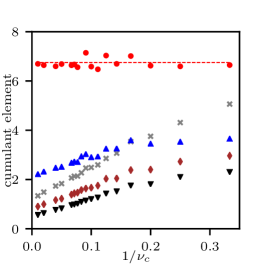
(b) Various $\nu_{c}$, constant $\sigma=0.5$ between all marginals.

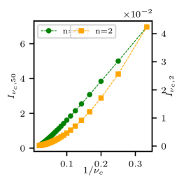
(c) The addtional mutual information $I_{\nu_{c},n}$, see Equation (13).

Figure 1: Elements of the $4$th cumulant tensor and mutual information for the t-Student copula parametrised by $\nu_{c}$ and $\sigma$ -the parameter of the cross-correlation between all marginals. t-Student univariate marginals with $\nu_{u}=6$ parameter were used for all marginals. The case $\frac{1}{\nu_{c}}\rightarrow 0$ refers to the Gaussian copula.

2.3 The analytical tools

For the practical reason of the outliers detection for the financial data, the projection of data onto directions with high values of the given higher-order cumulant is used. For this reason, the Higher Order Singular Value Decomposition (HOSVD) [41] of the higher order cumulants tensor can be used, see [22] for moment approach on financial data. For the review of other methods of tensor decomposition (including algorithmic implementation) see [54, 55].

Following [41, 53] and the discussed symmetry of the cumulant tensor (multi-index permutation invariance) such decomposition can be performed by the eigenvalue decomposition of the particular matrix. Let $c$ be the element of $\mathcal{C}_{d}$, its contraction with itself in $d-1$ modes gives the symmetric, (semi) positively defined matrix $\mathbf{M^{(d)}}\in\mathbb{R}^{n\times n}$,

$$m^{(d)}_{j_{1},j_{2}}=\sum_{i_{2},\ldots,i_{d}=1,\ldots,1}^{n,\ldots,n}c_{j_{1},i_{2},\ldots,i_{d}}\cdot c_{j_{2},i_{2},\ldots,i_{d}}.$$ (18)

Due to the mentioned symmetry, it is not important in which modes the contraction is performed, hence the matrix $\mathbf{M^{(d)}}$ is uniquely defined. By laborious element-wise operations one can show that the eigenvalues/eigenvectors decomposition of $\mathbf{M^{(d)}}=\mathbf{W}\mathbf{D}\mathbf{W}^{\intercal}$ corresponds to the HOSVD of the original tensor $\mathcal{C}_{d}$, given it is symmetric, here the matrix $\mathbf{D}$ is the diagonal matrix of non-negative eigenvalues of $\mathbf{M^{(d)}}$.

Further, following [41], it can be shown that if the eigenvalues in $\mathbf{D}$ are ordered from highest to lowest, the first columns of $\mathbf{W}$ (that are orthonormal) project data on the directions with high absolute value of the $d$-order cumulant. By analogy, the last columns of $\mathbf{W}$ project data onto the directions with low absolute value of the $d$-order cumulant. The second observation was used in [21], for the determination of portfolios of financial data with low variability for the crisis. In [21], the modification was made to construct the projection of data on the directions where the cumulants of subsequent order have all low absolute values to minimise the risk.

However, in the current approach, the analysis concentrates on the directions with absolute value of the $4$th order cumulant, to detect the crisis data that are supposed to be modelled by the t-Student copula.

3 The outliers detection

Let us represent $t$ realisations of $n$ variate data in the following matrix form: $\mathbf{X}\in\mathbb{R}^{t\times n}$. The subset of outliers realisations of size $\tau$ is approximately an order of magnitude smaller than the size of data ($t$). In this scenario, the outliers are expected to have the different probabilistic model than the ordinary data. For the outliers detection, the author will use the $4$th order multivariate cumulant outlier detector (the modified detector form [43]), and the state of art Reed-Xiaoli (RX) detector [56, 57]. For the current review of outlier detectors see [58]. here, it was pointed out that out of automatic (unsupervised) detectors the standard deviation based ones, such as the RX detector, are most frequently used. Moreover, the author’s intention is to demonstrate the information tied to the non-Gaussian joint distribution hence, the comparison with the RX detector, based on the mean vector and the covariance matrix, is straightforward.

3.1 The Reed-Xiaoli Detector

In theory, the RX detector requires the ordinary data (sometimes called the background) to follow the Gaussian multivariate distribution with the fixed covariance matrix and mean vector. Outliers are supposed to be modelled by the Gaussian distribution with the same covariance, but different mean vector. Nevertheless, the RX detector is applicable to analyse non-Gaussian distributed data as well, see for example [59] and references therein.

To introduce the RX detector, suppose the $j$^th realisation of data is represented in the vector form $\mathbf{x}_{j}\in\mathbb{R}^{n}$. Having estimated the mean vector $\mu$ and the covariance matrix $\mathcal{C}_{2}$ from data, we can calculate the Mahalanobis distance [60] between the given realisation and the mean vector:

$$md_{j}=(\mathbf{x}_{j}-\mu)\mathcal{C}_{2}^{-1}(\mathbf{x}_{j}-\mu)^{\intercal}.$$ (19)

The higher the value of $md_{j}$, the higher probability that the $j$^th realisation is an outlier.

Given the mentioned Gaussian assumptions, one can use the percentile of the $\chi^{2}$ squared distribution with $n$ degrees of freedom for the threshold value, to decide whether the analysed piece of data is an outlier or not. This representation is not straightforward if data are non-Gaussian distributed. However, here one can still use the threshold parameter, but without the ‘elegant’ probabilistic interpretation. Please note that, that the Mahalanobis distance appears in practice as a part of many detectors of outliers that are not necessarily Gaussian distributed [61, 62].

3.2 The $4$th order multivariate cumulant outlier detector

As the higher order multivariate cumulants are supposed to carry information about outliers, these cumulants may be used for an outlier detection. For this end the modification of the outlier detection algorithm from [43] is proposed. The original procedure can be summarised in the following steps.

1. Remove the mean vector and the standard cross-correlation from data $\mathbf{X}\rightarrow(\mathbf{X}-\mu)\mathcal{C}_{2}^{-\frac{1}{2}}$.

2. Project data onto directions with the highest and the lowest $4$th order moment.

3. Compute the distance between each realisation of the projected data and its median.

4. If the distance is higher than the threshold, remove the sample from data and move it to the outliers candidates set.

5. Continue the procedure as long as the stop condition is fulfilled, i.e. no more outliers candidates appear or the size of the set of outliers candidates is roughly a half of the data size.

6. Use the RX detector with the parameters estimated from the data subset without some outliers candidates, to detect true outliers. The detection threshold is the $99$th percentile of the corresponding $\chi^{2}$ distribution.

In [63] the procedure was modified by adding some additional random directions to the specific directions.

The author’s modification of the original outliers detection algorithm in [43], is presented in Algorithm 1. The modification concerns basically the replacement of the $4\textsuperscript{th}$ order moment by the $4\textsuperscript{th}$ order cumulant as being more informative for the financial data model discussed in this paper, see Subsection 2.2. Hence, the author proposes to project data onto the directions with the highest absolute value of the $4\textsuperscript{th}$ order cumulant, see Subsection 2.3. Observe that low absolute value of the $4$th cumulant is supposed to reefer to the Gaussian multivariate model, far from the model of the financial crisis.

Further, the author skips the RX detection in the last step of the outliers detection and the outliers candidate intermediate step. This is because both probabilistic models of data and outliers are non-Gaussian, hence the RX threshold parameter can not be simply estimated from the $\chi^{2}$ distribution. Further, the detector becomes simpler and is parametrised by only one parameter.

The last modification concerns the stop condition given no intermediate step of the outliers candidates. The stop condition must ensure that the small subset of data can be detected as outliers. For this sake, the author proposes the mean squared Kurtosis over specific directions. The iterative removal of outliers is being performed as long as such Kurtosis of remaining ordinary data is dropping.

Algorithm 1 the $4$th order multivariate cumulant outliers detection.

1:Input: $\mathbf{X}\in\mathbb{R}^{t\times n}$ - data, $\beta$ - the sensitivity parameter, $r$ - the number of specifics directions.

2:Output: outliers $\subset(1:t)$.

3:function hosvdc4detect($\mathbf{X}$, $\beta$, $r$)

4:     $\mathbf{X}=\mathbf{X}-\mu$ $\triangleright$ remove the mean vector

5:     $\mathbf{X}=\mathbf{X}\mathcal{C}_{2}^{-\frac{1}{2}}$ $\triangleright$ remove standard cross-correlations, $\mathcal{C}_{2}$ - the covariance matrix

6:     while $k_{\text{this step}}<k_{\text{previous step}}$ do

7:         compute $\mathcal{C}_{4}(\mathbf{X})$ and $\mathbf{M^{(4)}}$ $\triangleright$ see Eq. (18)

8:         $W_{1},\ldots,W_{r}=\text{eigenvec}\left(\mathbf{M^{(4)}}\right):\lambda_{1}\geq\ldots\geq\lambda_{n}$ $\triangleright$ $W_{i}\in\mathbb{R}^{n}$

9:         $Z_{1}=\left(W_{1}^{\intercal}\right)\mathbf{X},\ldots,Z_{r}=\left(W_{r}^{\intercal}\right)\mathbf{X}$

10:         $k=\sqrt{\sum_{i=1}^{r}\left(\text{kurtosis}(Z_{i})\right)^{2}}$

11:         for $j\leftarrow 1\textrm{ to (number of samples left)}$ do

12:              if $\max_{i}\frac{|z_{j,i}-\text{median}(Z_{i})|}{\text{MAD}(Z_{i})}>\beta$ then $\triangleright$ $z_{j,i}$ is $j$^th element of $Z_{i}$, MAD is the Median Absolute Deviation

13:                  append $j$ to outliers

14:              end if

15:         end for

16:         Remove outliers realisations from $\mathbf{X}$

17:     end while

18:     return outliers

19:end function

3.3 Experiments on artificial data

The artificial data are designed to mimic, at least to some extend, the financial data. Hence following [16] the univariate marginals with the asymptotic power law tails are selected. For the particular analysis the t-Student univariate marginals, see Eq. (11), are selected. As mentioned before the parameter of the marginals is $\nu_{u}=6$. Data size is proposed to be $t=1000$ corresponding to a few trading years or the size of the longest observation window in [11]. The number of marginals is set to $n=30$, which corresponds to the size of the typical market index. Data are divided onto the outliers subset of size $\tau=0.1t$ and the ordinary data subset of size $t-\tau$. One can expect the crisis periods to be of an order of magnitude shorter than the normal periods. Following, the discussion in the Introduction and Section 2 the ordinary data are expected to have zero tail dependencies (simultaneous extreme events are not possible). On the contrary, the crisis data are expected to have the meaningfully positive tail dependencies between some marginals (there may be still the subset of safe assets). Hence, for modelling the ordinary data, the Gaussian copula is selected while for modelling the crisis data the t-Student copula for the subset containing one half of the marginals and the Gaussian copula for the rest of the marginals. The correlation matrix is randomly generated and is expected to be similar for ordinary data and the outliers.

The artificial data generation scheme uses the modified t-Student distributed data generator [48]. The algorithm is implemented in the Julia programming language [44] and available on the GitHub repository [46] as the function gcop2tstudent(). It is summarised in the following points.

1. Randomly generate the correlation matrix $\Sigma$, by means of the ’random’ method from [64] - function cormatgen_rand() in [46].

2. Generate $t$ realisations of $n$-variate Gaussian distribution parametrised by $\Sigma$.

3. For the randomly selected subset of marginals of size $n/2$, transform multivariate Gaussian distribution into the t-Student one (parametrised by $\nu_{c}$) by multiplying all elements of each realisation by $\sqrt{\frac{\nu_{c}}{v_{0}}}$, where $v_{0}\sim\chi^{2}_{\nu_{c}}$.

4. Transform all univariate marginals to the desirable ones, i.e. the t-Student with the parameter $\nu_{u}$.

Although, the sampling from $\chi^{2}_{\nu_{c}}$ slightly decreases the cross-correlation between two subsets of marginals (see point $3$), the effect decreases with the rise of $\nu_{c}$, and correlation matrices of the ordinary data ($\Sigma_{\text{ordinary}}$) and the outliers ($\Sigma_{\text{outliers}}$) are similar, the maximal difference rarely exceeds $0.1$, see Figure 2.

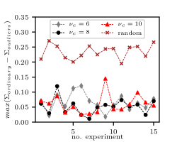
Figure 2: Maximal differences between the correlation matrix of the ordinary data $\Sigma_{\text{ordinary}}$ and the outliers $\Sigma_{\text{outliers}}$, in both cases $100$ samples were taken. Random means twice sample the $\Sigma$ matrices by means of the ’random’ method from [64] equivalently the function cormatgen_rand() [46].

The example realisations of the detection are presented in Figure 3, for more examples run tests in ./test/outliers_detect/ of [45]. The results are presented in the form of the ROC (Receiver Operating Characteristic) curve. The True Positive Rate is the rate of truly detected outliers out of all outliers. The False Positive Rate is the rate of the type one error (the number of the falsely detected data over the number of the ordinary data).

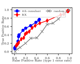
(a) $\nu_{c}=6$

(b) $\nu_{c}=8$

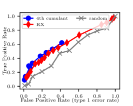
(c) $\nu_{c}=10$

Figure 3: Exemplary detections of artificial outliers. One can see that the $4$th cumulant outperforms both the RX and the random choice. Although the $4$th cumulant method does not fully cover the detection range, the performance is similar to the mentioned further example of the financial crisis detection. For the cumulant method the number of specific directions parameter was chosen to be $r=3$.

The $4$th cumulant method outperforms the RX and the random choice. It does not fully cover the detection range, but it can assure the $60-80\%$ True Positive Rate for the low False Positive Rate. In the author’s opinion, the advantage over the RX detector comes from the limitations concerning the use of the Mahalanobis distance in the RX detector for the non-Gaussian distributed data.

4 Financial data analysis

In this section, the application of the outlier detection on the real life financial data is discussed. The goal of the analysis concerns the crisis detection and the crisis prediction in the equity markets. For the data representation, individual assets correspond to marginals and their log increases correspond to the realisations. The assets are share prices of important companies traded on two distinct stock exchanges: the large New York Stock Exchange and the medium size Warsaw Stock Exchange. The reason for such selection of data is that one may expect different dynamics of the large well-developed market in comparison to the dynamics of the medium-size, not fully developed market. In both cases, the analysis concerns the data from approximately $270$ trading days, that covers the whole trading year. In both cases, the author selected the period when the increase of the index value was followed by the crisis, i.e.: for the New York Stock Exchange January 2017 - February 2018, see Figure 4(a); for the Warsaw Stock Exchange June 2010 - August 2011, see Figure 5(a). To increase the number of data for statistics, two records per day are taken: the opening price and the closing price.

The input data are the log increments of the share prices of the companies included in the relevant stock exchange index. In the case of the New York Stock Exchange, the Dow Jones Industrial (DJI) index containing $30$ major companies is used. Due to the data availability, the analysis is limited to the $29$ following companies: AAPL, BA, CSCO, DIS, GS, IBM, JNJ, KO, MMM, MSFT, PFE, TRV, UTX, VZ, WMT, AXP, CAT, CVX, DWDP, HD, INTC, JPM, MCD, MRK, NKE, PG, UNH, V, WBA. In the case of the Warsaw Stock Exchange, the WIG20 index containing $20$ major companies is used. Analogically, due to the data availability, the analysis is limited to the $19$ following companies: ASSECOPOL, CEZ, GTC, KERNEL, LOTOS, ORANGEPL, PEKAO, PGNIG, PKOBP, TAURONPE, BOGDANKA, GETIN, HANDLOWY, KGHM, MBANK, PBG, PGE, PKNORLEN, PZU.

For the crisis detection, scenario the observation window includes mostly ordinary trading, but ends on the crisis data, see Figure 4(a) and Figure 5(a). The size in the observation window covers the whole trading year, hence the seasonal fluctuations of the ordinary data are accounted for. The crisis data were selected manually, looking for sharp drops of the index values. Ordinary and crisis data are separated by the red vertical lines in Figure 4(a) and Figure 5(a).

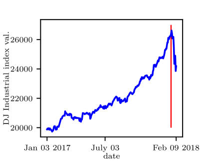
(a) The DJI index, the red line marks the start of the crisis at January 25, 2018.

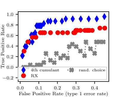
(b) The crisis detection performance, for the cumulant method used $r=3$ specific directions.

Figure 4: The crisis detection on New York Stock Exchange. The red vertical line splits data between the ordinary data and the crisis data.

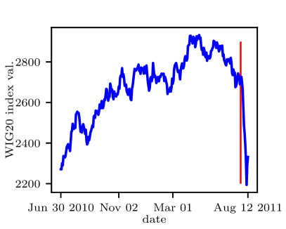
(a) The WIG20 index, the red line marks the start of the crisis at July 28, 2011.

(b) The crisis detection performance, for the cumulant method used $r=3$ specific directions.

Figure 5: The crisis detection on Warsaw Stock Exchange. The red vertical line splits data between the ordinary data and the crisis data.

The analysis of the crisis detection performance is presented in Figure 4(b) and Figure 5(b), where the True Positive Rate of the detection is plotted against the False Positive Rate being the rate of the type one error. In most cases the $4$th cumulant algorithm outperforms the RX detector. Hence, both for WIG20 and DJI data, the higher-order cumulant (of order $4$ in this case) can play the meaningful role in the crisis detection. Given the False Positive Rate a bit higher than $0.1$ the True Positive Rate of the $4$th cumulant algorithm is large and the crisis can be detected with high probability after recording one piece of the crisis data. This region corresponds to the detectors sensitively parameter roughly fulfilling $\beta\leq 2.5$, see Algorithm 1. However, as the $\beta$ parameter drops, the False Positive rate rises.

Furthermore, referring to Figure 5, the performance of the crisis detection on the Warsaw Stock Exchange appears to be similar to the detection of outliers artificially sampled by means of the t-Student copula, see Figure 3. Hence, the t-Student copula appears to be a good model of the crisis data of the medium size stock exchange. Referring to the New York Stock Exchange case, the performance of the $4$th cumulant is even better. This may suggest higher cross-correlation of extreme events for the examined crisis on the New York Stock Exchange. However, since the $4$th cumulant measures the information tied to the t-Student copula (see Section 2) the t-Student copula (or perhaps its generalisation) should be considered as the crisis data model here as well.

(a) The WIG20 index, the green line marks the start of the period directly preceeding the crisis (July 11, 2011), the red line marks the start of the crisis (July 28, 2011).

(b) The crisis prediction, $r=3$.

Figure 6: The crisis prediction on Warsaw Stock Exchange. The range with the low False Positive Rate was chosen, since we have the sequence of pre-crisis data to make a proper detection. The advantage of the $4$th cumulant is for False Positive Rate smaller than the $0.1$, that correspond to the parameter $\beta\geq 2.75$.

Since the Warsaw Stock Exchange example fits to the theoretical model, it will be chosen for the crisis prediction scenario. In this scenario, the green line separates the ordinary data from the outliers (crisis predecessors), see Figure 6. Hence, there are several pre-crisis events available before the crisis occurs, one should concentrate rather on the low False Positive Rate. In this region, the $4$th cumulant outperforms the RX detector, see Figure 6(b).

5 Conclusions

Given the analysis of the New York Stock Exchange and the Warsaw Stock Exchange, one can conclude that the $4$th order multivariate cumulants are applicable in the crisis detection scenario both on large and medium sized stock exchanges. These cumulants measure the cross-correlation of the extreme events, what appears during the crisis. Such extreme events can be modelled by the t-Student copula that is informatively tied to $4$th order multivariate cumulants. Due to the analogy in outliers detection scheme, the t-Student copula is best applicable to model the crisis on the medium sized stock exchanges such as the Warsaw Stock Exchange.

Interesting aspect concerns the feasibility of the $4$th order multivariate cumulants in the crisis prediction. Here, positive results for the Warsaw Stock Exchange rise the suggestion that in analogy to the auto-correlated extreme events, the cross-correlated extreme events may appear before the crisis. Since the cumulant based outliers detector does not look into the auto-correlation of financial data it may support the Hurst Exponent based methods looking into auto-correlation of these data for crisis prediction.

Acknowledgments

The research was partially financed by the National Science Centre, Poland – project number 2014/15/B/ST6/05204. The author would like to thank Jarosław Adam Miszczak for revising the manuscript and discussion and Adam Glos for an implementation assistance.

References

- [1] J.-P. Bouchaud, M. Potters, Theory of Financial Risks and Derivative Pricing. From Statistical Physics to Risk Management, Cambridge University Press, (2nd Edition), 2003.
- [2] V. Akgiray, Conditional Heteroscedasticity in Time Series of Stock Returns: Evidence and Forecasts, J. Bus. (1989) 55–80.
- [3] G. L. Vasconcelos, A guided walk down Wall Street: an introduction to econophysics, Brazilian Journal of Physics 34 (3B) (2004) 1039–1065. doi:10.1590/S0103-97332004000600002.
- [4] R. Matsushita, P. Rathie, S. Da Silva, Exponentially damped Lévy flights, Physica A: Statistical Mechanics and its Applications 326 (3-4) (2003) 544–555. doi:10.1016/S0378-4371(03)00363-7.
- [5] N. Vandewalle, M. Ausloos, Coherent and random sequences in financial fluctuations, Physica A: Statistical Mechanics and its Applications 246 (3-4) (1997) 454–459. doi:10.1016/S0378-4371(97)00366-X.
- [6] P. Grau-Carles, Empirical evidence of long-range correlations in stock returns, Physica A: Statistical Mechanics and its Applications 287 (3-4) (2000) 396–404. doi:10.1016/S0378-4371(00)00378-2.
- [7] B. B. Mandelbrot, Fractals and scaling in finance: Discontinuity, concentration, risk. Selecta volume E. Springer Science & Business Media (2013).
- [8] N. Vandewalle, P. Boveroux, A. Minguet, M. Ausloos, M, The crash of October 1987 seen as a phase transition: amplitude and universality. Physica A: Statistical Mechanics and its Applications, 255 (1998), 201–210. doi:10.1016/S0378-4371(98)00115-0.
- [9] D. Grech, G. Pamuła, The local hurst exponent of the financial time series in the vicinity of crashes on the polish stock exchange market, Physica A: statistical mechanics and its applications 387 (16-17) (2008) 4299–4308. doi:10.1016/j.physa.2008.02.007.
- [10] D. Grech, Z. Mazur, Can one make any crash prediction in finance using the local hurst exponent idea?, Physica A: Statistical Mechanics and its Applications 336 (1-2) (2004) 133–145. doi:10.1016/j.physa.2004.01.018.
- [11] K. Domino, The use of the Hurst exponent to predict changes in trends on the Warsaw Stock Exchange, Physica A: Statistical Mechanics and its Applications 390 (1) (2011) 98–109. doi:10.1016/j.physa.2010.04.015.
- [12] K. Domino, The use of the Hurst exponent to investigate the global maximum of the Warsaw Stock Exchange WIG20 index, Physica A: Statistical Mechanics and its Applications 391 (2012) 156–169. doi.org/10.1016/j.physa.2011.06.062.
- [13] R. Rak, D. Grech, Quantitative approach to multifractality induced by correlations and broad distribution of data, Physica A: Statistical Mechanics and its Applications 508 (2018) 48–66. doi:10.1016/j.physa.2018.05.059.
- [14] P. Bak, M. Paczuski, M. Shubik, Price variations in a stock market with many agents, Physica A: Statistical Mechanics and its Applications 246 (3-4) (1997) 430–453. doi:10.1016/S0378-4371(97)00401-9.
- [15] N. Kruszewska, P. Weber, A. Gadomski, and K. Domino, A method of mechanical control of structure-property relationship in grains-containing material systems, Acta Physica Polonica B 44, no. 5 (2013): 1049-1066. doi:10.5506/APhysPolB.44.1049
- [16] D. Sornette, Dragon-kings, black swans and the prediction of crises, arXiv preprint arXiv:0907.4290 (2009).
- [17] B. V. de Melo Mendes, R. M. de Souza, Measuring financial risks with copulas, International Review of Financial Analysis 13 (1) (2004) 27–45. doi:10.1016/j.irfa.2004.01.007.
- [18] G. Szegö, Measures of risk, Journal of Banking & Finance 26 (7) (2002) 1253–1272. doi:10.1016/S0378-4266(02)00262-5.
- [19] R. S. Calsaverini, R. Vicente, An information-theoretic approach to statistical dependence: Copula information, EPL (Europhysics Letters) 88 (6) (2009) 68003. doi:10.1209/0295-5075/88/68003.
- [20] D. Sornette, P. Simonetti, J. Andersen, -field theory for portfolio optimization: “fat tail” and nonlinear correlations, Physics Report 335 (2000) 19–92. doi:10.1016/S0370-1573(00)00004-1.
- [21] K. Domino, The use of the multi-cumulant tensor analysis for the algorithmic optimisation of investment portfolios, Physica A: Statistical Mechanics and its Applications 467 (2017) 267–276. doi:10.1016/j.physa.2016.10.042.
- [22] M. Rubinstein, E. Jurczenko, B. Maillet, Multi-moment asset allocation and pricing models, Vol. 399, John Wiley & Sons, 2006.
- [23] M. Sawa, D. Grech, Alternative Random Matrix Approach in Analysis of Correlations in Financial Data, Acta Physica Polonica A (2015), 127(3A). doi:10.12693/APhysPolA.127.A-118
- [24] G. Cao, L. Y. He, J. Cao, Multifractal Detrended Analysis Method and Its Application in Financial Markets, (2018) Springer. doi:10.1007/978-981-10-7916-0_4
- [25] L. Y. He, S. P. Chen, Multifractal detrended cross-correlation analysis of agricultural futures markets. Chaos, Solitons & Fractals, (2011) 44(6), 355-361. doi:/10.1016/j.chaos.2010.11.005
- [26] U. Cherubini, E. Luciano, W. Vecchiato, Copula methods in finance, John Wiley & Sons, 2004.
- [27] K. Domino, T. Błachowicz, The use of copula functions for modeling the risk of investment in shares traded on the Warsaw Stock Exchange, Physica A: Statistical Mechanics and its Applications 413 (2014) 77–85. doi:10.1016/j.physa.2014.06.083.
- [28] K. Domino, T. Błachowicz, The use of copula functions for modeling the risk of investment in shares traded on world stock exchanges, Physica A: Statistical Mechanics and its Applications 424 (2015) 142–151. doi:10.1016/j.physa.2015.01.019.
- [29] R. B. Nelsen, An Introduction to Copulas, Springer, Science & Business Media, 2007.
- [30] M. Semenov, D. Smagulov, Copula Models Comparison for Portfolio Risk Assessment, In Global Economics and Management: Transition to Economy 4.0 (2019) pp. 91-102, Springer, Cham. https://doi.org/10.1007/978-3-030-26284-6_9 doi:10.1007/978-3-030-26284-6_9
- [31] M. Opper, D. Saad, Advanced mean field methods: Theory and practice, MIT press, 2001.
- [32] R. O. Duda, P. E. Hart, D. G. Stork, Pattern classification, John Wiley & Sons, 2012.
- [33] P. McCullagh, Tensor methods in statistics, Vol. 161, Chapman and Hall London, 1987.
- [34] M. G. Kendall, et al., The advanced theory of statistics., The advanced theory of statistics. (1946).
- [35] K. Domino, P. Gawron, Ł. Pawela, Efficient Computation of Higher-Order Cumulant Tensors, SIAM Journal on Scientific Computing 40 (3) (2018) A1590–A1610. doi:10.1137/17M1149365.
- [36] J. C. Arismendi, H. Kimura, Monte Carlo Approximate Tensor Moment Simulations, Available at SSRN 2491639 (2014).
- [37] E. Jondeau, E. Jurczenko, M. Rockinger, Moment component analysis: An illustration with international stock markets, Journal of Business & Economic Statistics 36 (4) (2018) 576–598. doi:10.1080/07350015.2016.1216851.
- [38] P. Eckhard, and R. Rendek, Empirical evidence on Student-t log-returns of diversified world stock indices, Journal of statistical theory and practice 2.2 (2008): 233-251. doi.org/10.1080/15598608.2008.10411873
- [39] P. J. Cayton, D. Mapa, et al., Time-varying conditional Johnson Su density in Value-at-Risk methodology, Philippine Review of Economics 52 (1) (2015) 23–44.
- [40] S. T. Rachev, Handbook of heavy tailed distributions in finance: Handbooks in finance, Vol. 1, Elsevier, 2003.
- [41] L. De Lathauwer, B. De Moor, J. Vandewalle, A multilinear singular value decomposition, SIAM journal on Matrix Analysis and Applications 21 (4) (2000) 1253–1278. doi:10.1137/S0895479896305696.
- [42] K. Domino, P. Gawron, An algorithm for arbitrary-order cumulant tensor calculation in a sliding window of data streams, Int. J. Appl. Math. Comput. Sci 29 (1) (2019) 195–206. doi:10.2478/amcs-2019-0015.
- [43] D. Peña, F. J. Prieto, Multivariate outlier detection and robust covariance matrix estimation, Technometrics 43 (3) (2001) 286–310. doi:10.1198/004017001316975899.
- [44] J. Bezanson, A. Edelman, S. Karpinski, V. B. Shah, Julia: A fresh approach to numerical computing, SIAM Review 59 (1) (2017) 65–98. doi:10.1137/141000671.
- [45] K. Domino, CumulantsFeatures.jl, https://github.com/iitis/CumulantsFeatures.jl (2020). doi:10.5281/zenodo.3676928.
- [46] K. Domino, A. Glos, DatagenCopulaBased.jl, https://github.com/iitis/DatagenCopulaBased.jl (2020). doi:10.5281/zenodo.3676933.
- [47] A. Sklar, Fonctions de répartition á n dimensions et leurs marges, Publ. Inst. Statist. Univ. Paris, (1959) 8: 229–231.
- [48] S. Kotz, S. Nadarajah, Multivariate t-distributions and their applications, Cambridge University Press, 2004.
- [49] S. Kullback, R. A. Leibler, On information and sufficiency, The annals of mathematical statistics 22 (1) (1951) 79–86.
- [50] I. W. Martin, Consumption-based asset pricing with higher cumulants, The Review of Economic Studies 80 (2) (2013) 745–773. doi:10.1093/restud/rds029.
- [51] P. McCullagh, J. Kolassa, Cumulants, Scholarpedia 4 (3) (2009) 4699.
- [52] N. Balakrishnan, N. L. Johnson, S. Kotz, A note on relationships between moments, central moments and cumulants from multivariate distributions, Statistics & probability letters 39 (1) (1998) 49–54. doi:10.1016/S0167-7152(98)00027-3.
- [53] L. R. Tucker, Some mathematical notes on three-mode factor analysis, Psychometrika 31 (3) (1966) 279–311.
- [54] M. D. Schatz, T. M. Low, R. A. van de Geijn, T. G. Kolda, Exploiting symmetry in tensors for high performance: Multiplication with symmetric tensors, SIAM Journal on Scientific Computing 36 (5) (2014) C453–C479. doi:10.1137/130907215.
- [55] T. G. Kolda, B. W. Bader, Tensor decompositions and applications, SIAM review 51 (3) (2009) 455–500. doi:10.1137/07070111X.
- [56] I. S. Reed, X. Yu, Adaptive multiple-band CFAR detection of an optical pattern with unknown spectral distribution, IEEE Transactions on Acoustics, Speech, and Signal Processing 38 (10) (1990) 1760–1770. doi:10.1109/29.60107.
- [57] C.-I. Chang, S.-S. Chiang, Anomaly detection and classification for hyperspectral imagery, IEEE transactions on geoscience and remote sensing 40 (6) (2002) 1314–1325. doi:10.1109/TGRS.2002.800280.
- [58] J. Yang, S. Rahardja, P. Franti, Outlier detection: how to threshold outlier scores?. (2019, December). In Proceedings of the International Conference on Artificial Intelligence, Information Processing and Cloud Computing (pp. 1-6). doi.org/10.1145/3371425.3371427.
- [59] P. Głomb, M. Romaszewski, M. Cholewa, K. Domino, Application of hyperspectral imaging and machine learning methods for the detection of gunshot residue patterns, Forensic science international 290 (2018) 227–237. doi:10.1016/j.forsciint.2018.06.040.
- [60] M. P. Chandra, et al., On the generalised distance in statistics, in: Proceedings of the National Institute of Sciences of India, Vol. 2, 1936, pp. 49–55.
- [61] R. Das, B. K. Sinha, et al., Detection of multivariate outliers with dispersion slippage in elliptically symmetric distributions, The Annals of Statistics 14 (4) (1986) 1619–1624.
- [62] B. K. Sinha, Detection of multivariate outliers in elliptically symmetric distributions, The Annals of Statistics (1984) 1558–1565.
- [63] D. Peña, F. J. Prieto, Combining random and specific directions for outlier detection and robust estimation in high-dimensional multivariate data, Journal of Computational and Graphical Statistics 16 (1) (2007) 228–254. doi:10.1198/106186007X181236.
- [64] K. Domino, A. Glos, Introducing higher order correlations to marginals’ subset of multivariate data by means of Archimedean copulas, arXiv preprint arXiv:1803.07813 (2018).