Cone types and asymptotic invariants for the random walk on the modular group
Abstract.
We compute the cone types of the Cayley graph of the modular group associated with the standard system of generators . We do this by showing that, in general, there is a set of suffixes of each element that completely determines the cone type of the element, and such suffixes are subwords of primitive relators.
Then, using J. W. Cannon’s seminal ideas (1984), we compute its growth function. We estimate from above and below the spectral radius of the random walk using ideas from T. Nagnibeda (1999) and S. Gouëzel (2015). Finally, using results of Y. Guivarc’h (1980) and S. Gouëzel, F. Mathéus and F. Maucourant (2015), we estimate other asymptotic invariants of the random walk, namely, the entropy and the drift.
1. Introduction
The modular group is arguably one of the most fundamental groups in mathematics and, accordingly, one of the most studied.
In this note we study through the lens of combinatorial and geometric group theory, focusing on the asymptotic invariants for the (simple symmetric) random walk on the Cayley graph of associated with the standard generators and .
It is worth to mention that is also the free product of the cyclic groups generated by and , of order two and three, respectively. Thus, we have the presentation . From the combinatorial and geometric group theoretic view point, this presentation is the handier. In fact, the invariants for associated with the generators and can be computed explicitly, as we survey in the Appendix A.
We focus our attention in the generators and as they do not allow such straightforward computations but are still of interest. In fact, they are geometrically meaningful as orbifold fundamental curves on the modular curve (as it is also the case for the generating set , which we address in Appendix B). Our case of study is also of interest from the combinatorial and geometric group theoretic point of view, since it is still a Cayley graph of a free product of two cyclic groups, but with respect to a generating set different from the ones that have been well understood.
We base our method on J. W. Cannon’s classification of group elements by their cone types and our main contribution is the computation of the cone types of relative to . This allows to compute the growth series using Cannon’s original ideas [Cannon], and to give numerical estimates for the spectral radius of the random walk using ideas from T. Nagnibeda [Nagnibeda] and S. Gouëzel [Gouezel]. We also estimate the entropy and the drift of the random walk applying a result of S. Gouëzel, F. Mathéus and F. Maucourant [Gouezel-Matheus-Maucourant].
One motivation for writing this note is that, even if it is likely that in the present case estimates (or even a complete description; cf. Appendix A) may be known by experts, we could not find any clue in the literature. On the other hand, this work arises as a spin-off of [Pardo:quantitative, Appendix B], where we compute cone types for a different Fuchsian group in order to apply Nagnibeda’s ideas and give lower bounds for the bottom of the spectrum of the combinatorial Laplace operator, which is equivalent to estimates from above for the spectral radius of the corresponding random walk, as shows (1) below. In particular, there is some text overlap in respect to some background material. We also stress that the estimates in the present work do not intend to be optimal in any sense.
1.1. Cone types
For a set , we denote by the free monoid on , an element in is called a word in , and the elements in are the letters.
For a system of generators of a group , in a slight abuse of notation we still write for . There is a natural evaluation morphism , that associates to a word the product of its letters in . We denote the length of an element of by , that is, the number of its letters. Similarly, we denote by the word length in associated with . That is, for an element , . We say that is a geodesic if . We also denote inversion by an overbar, that is, if , then and, if , where , then .
Given , the cone of relative to , denoted , is the set of for which some geodesic from to passes through , that is,
For each element , its cone naturally defines a rooted subgraph of the Cayley graph. We say that two cones are equivalent (or, of the same type) if they are isomorphic as rooted graphs. The cone type of (relative to ) is the equivalence class of , which, in a slight abuse of notation, we still denote by .
It follows from Cannon’s work that if is a word-hyperbolic group —as is the case of the modular group —, then there are only finitely many cone types [Cannon, Corollary 2]. Our proof follows the same lines but does not depend on this result, however.
Theorem 1.1 (Cone types).
Let and . Then, there are exactly six cone types: , , , , and .
Furthermore, we give a simple combinatorial description for each cone type in Section 3. On the other hand, in the proof of Theorem 1.1 arises the following general phenomenon of independent interest.
Theorem 1.2.
Let be a group generated by a finite system and suppose that the set of primitive relators (over ) is finite. Then, has finitely many cone types (relative to ).
Here, by relator we mean a word in that evaluates to the identity and by primitive, that it does not contain proper subwords that are also relators.
In fact, we show in Proposition 2.5, that for any group and generating system , the set of all maximal suffixes of geodesics for that are subwords of a primitive or trivial relator completely determines the cone type of . In particular, knowing the set of primitive relators allows to compute, algorithmically at least, every cone type.
1.2. Growth
For , let be the sphere of radius , that is, . The (spherical) growth series of relative to is then the formal series
It follows from Cannon’s work that if has finitely many cone types relative to , then the growth series corresponds to a rational analytic function [Cannon, Theorem 7] and the reciprocal of its radius of convergence gives the rate of exponential growth of the group relative to , denoted and also called growth, for short.
Theorem 1.3 (Growth).
Let and . Then, the growth series of relative to corresponds to the rational analytic function
In particular, the rate of exponential growth of relative to is the golden ratio, that is,
Remark 1.4.
In particular, the growth sequence corresponds to [oeis, A054886].
1.3. Random walk
The (right, simple symmetric) random walk on relative to is the Markov chain on whose transition probabilities are defined by
A realization of the random walk starting from the identity is given by and , where is an independent sequence of -valued uniformly distributed random variables. In other words, it is the (simple symmetric) random walk on the Cayley graph of relative to .
1.3.1. Spectral radius
We denote , the corresponding Markov operator, that is,
We denote the spectral radius of the random walk on relative to , that is, the spectral radius of ,
We estimate from above following ideas of Nagnibeda [Nagnibeda]. We also follow ideas of Gouëzel [Gouezel] to estimate from below. More precisely, we prove the following.
Theorem 1.5 (Spectral radius).
Let and . Then, the spectral radius of the random walk on relative to satisfies
Remark 1.6.
The spectral radius associated with a symmetric finite system of generators, is bounded from below by the spectral radius of (the random walk on) a regular tree of degree , that is, by (see, e.g., [ColinDeVerdiere, Chapter II, Section 7.2]). In our case, this yields . In particular, our estimates from below improves the trivial bound obtained by comparison to the regular tree.
It is also worth to mention that the spectral radius of relative to can be explicitly computed. In fact, (see Theorem A.3).
1.3.2. Bottom of the spectrum of the Laplace operator
A related quantity of interest is the bottom of the Laplace spectrum, which we denote . More precisely, let be the Laplace operator on relative to , that is,
Then is the bottom of the spectrum of , that is,
By definition, . Moreover, when the Cayley graph is bipartite —as is the case for and —, the spectrum of the Markov operator is symmetric. In such case, it follows that the bottom of the spectrum is related to the spectral radius by the formula
| (1) |
As a direct consequence of (1) and Theorem 1.5 we get the following.
Corollary 1.7 (Bottom of the Laplace spectrum).
Let and . Then, the bottom of the spectrum of the Laplace operator on relative to satisfies
Remark 1.8.
Compare with the trivial upper bound given by the regular tree of degree three, that is, . Also, compare with the bottom of the Laplace spectrum relative to : (see Corollary A.4).
1.3.3. Entropy and drift
Several numerical quantities have been introduced to describe the asymptotic behavior of random walks on groups (relative to a generating system). The spectral radius is one of them. Other important asymptotic invariants are the (asymptotic) entropy and the drift of the random walk. These are defined by
where is the uniform distribution on and , its -fold convolution. There is a fundamental inequality relating the entropy, the drift and the growth due to Guivarc’h [Guivarch]. Moreover, Gouëzel, Mathéus and Maucourant [Gouezel-Matheus-Maucourant] showed that estimates on the asymptotic invariants can be obtained from the others in several ways. This, together with Theorems 1.3 and 1.5, allows us to prove the following.
Theorem 1.9 (Entropy and drift).
Let and . Then, the entropy and the drift of the random walk on relative to satisfy
1.4. Comparison between the three generating systems
In Appendices A and B we study other two geometrically meaningful systems of generators of the modular group . Namely, and , where , and . Note that . For a schematic comparison, we summarize in Table 1 the results on the asymptotic invariants associated with these three generating systems.
| Growth | |||
|---|---|---|---|
| Spectral radius | |||
| Entropy | |||
| Drift |
1.5. Structure of the paper
In Section 2, we recall the basics of combinatorial group theory we need and prove some useful general combinatorial results. In particular, in Section 2.1 we prove Theorem 1.2.
In Section 3, we compute the cone types of relative to , proving Theorem 1.1, and use them to produce a recurrence for the growth series as in Cannon’s seminal work. We prove Theorem 3.3 in Section 3 and Theorem 1.3, in Section 3.2. We also include a graphical representation of the Cayley graph associated with in Figure 3.
In Section 4 we estimate the spectral radius . In Section 4.1, we state Nagnibeda’s ideas for the upper bounds and, in Section 4.2, those of Gouëzel, for the lower bounds. To conclude the proof of Theorem 1.5, we include some details of the computations for the lower bound in LABEL:sect:suffix-type and LABEL:sect:my-type.
In Section 5 we state Guivarc’h [Guivarch] and Gouëzel–Mathéus–Maucourant [Gouezel-Matheus-Maucourant] results relating the entropy and the drift to the growth and the spectral radius. Using our estimates for the spectral radius and the exact value of the growth , this allows us to estimate the entropy and the drift and prove Theorem 1.9.
In Appendix A we survey the analogous results in the case of the system of generators , which yields a presentation of as a free product of cyclic groups. In such case much more can be proven. In particular, we present the full Markov spectrum for the simple symmetric random walk in relative to and the exact values of the corresponding growth, spectral radius, entropy and drift. We also include a graphical representation of the Cayley graph associated with in Figure 4.
In Appendix B we repeat the study done for , for the system of generators . That is, we compute the growth series, estimate the spectral radius, the entropy and the drift of relative to . We also include a graphical representation of the Cayley graph associated with in LABEL:fig:Cayley-graph-2.
Acknowledgements
The author is grateful Sebastien Gouëzel for the reference to the work of T. Nagnibeda. The author is also greatly indebted to Tatiana Nagnibeda for useful comments and suggestions that improved the presentation of the paper, and for her patience providing him insight on the problems discussed in this work.
2. Combinatorial group theory
In this section, we recall the basics of combinatorial group theory we need and prove some useful general combinatorial results useful for our purposes.
The following discussion is completely general. For a complete introduction to this topic we refer the reader to Magnus–Karrass–Solitar’s book [Magnus-Karrass-Solitar].
Let be any group, and let be a subset of . A word in is any expression of the form
where and , . The number is the length of the word. The empy word, denoted , is the only one word of length zero. Given two words and , we say that is a subword of if , for some words and . If is the empty word we say that is a prefix of . If is the empty word we say that is a suffix of .
Each word in represents an element of . Namely, the product of the expression, which we denote . For example, the identity element can be represented by the empty word, that is, . We say that two words are equivalent if they represent the same element in .
Notation.
As usual, we use exponential notation for abbreviation; for example, the word can also be denoted by . We also use an overbar to denote inverses, thus stands for , and if , then .
In these terms, a subset of a group is a system of generators if and only if every element of can be represented by a word in . Henceforth, let be a fixed system of generators of and a word is assumed to be a word in . We say that a non-empty word is a relator if it represents the identity element of , that is, if it equivalent to the empty word. A generator next to its own inverse ( or ) define a trivial relator.
For a relator, we call a subword that is also a relator, a subrelator. We say that a word is reduced if it has no trivial subrelators. We say that a non-trivial relator is primitive if if it does not contain proper subrelators. In particular, a word is a geodesic if and only if it contains no primitive relators as subword. Note that, if is a system of generators and is the set of all primitive relators on , then is a presentation of .
For an element , we consider the word norm to be the least length of a word which represents when considered as a product in , and every such word is called a geodesic, that is, if its length coincides with its word norm when considered as a product in . A geodesic does not contains relators as subwords and, in particular, it is is always reduced. Also, a subword of a geodesic is also a geodesic.
The following decomposition result (see Figure 1) will be useful in Section 3 (in the form of Proposition 2.2 below).
Lemma 2.1.
Let be two different equivalent geodesics. Then, there are geodesics , and such that and , and is a primitive relator (of even length).
Proof.
Let be the largest common suffix of and (possibly is empty). Write and . Let and be the smallest non-empty suffixes of and respectively such that and are equivalent. Such and exist since and are different words. Moreover, they have the same length since they are equivalent geodesics, that is, they evaluate to the same element in . Write and (possibly and are empty). In particular and are equivalent, since the same holds for and . See Figure 1.
It remains to prove that is primitive. Suppose is a subrelator of . Since and are geodesics, their subwords are also geodesics and, therefore, they do not contain any relator as subword. It follows that for some non-empty suffixes and , of and , respectively. In particular, and are non-empty suffixes of and , respectively, and are equivalent. But, by definition, and are the smallest such suffixes and therefore and . Thus, has no proper subrelators and, therefore, is primitive. ∎
As a direct consequence of Lemma 2.1, we have the following.
Proposition 2.2.
Let and be two equivalent geodesics such that is also geodesic. Then, is a subword of some primitive relator (of even length).
Proof.
Consider the decomposition given by Lemma 2.1. It is clear that is a subword of and , of . Then is a subword of the primitive relator . ∎
2.1. Cone types
Recall that the cone of an element , relative to , is the set of for which some geodesic from to passes through . More precisely, let be the set of all geodesics for , that is, . Then,
Moreover, in a slight abuse of notation, we shall identify with the rooted graph that it defines as subgraph of the Cayley graph of . Finally, the cone type of an element is the isomorphism class of rooted graphs of .
To any rooted graph , one can associate its tree of geodesics, that is, the (rooted) tree where vertices are geodesics from the root of and edges correspond to length-increasing edges in . It is clear that isomorphic rooted graphs yield isomorphic trees of geodesics.
In particular, in order to study cone types it is worth to determine their tree of geodesics. A way to do this is through other type functions. A type function for (relative to ) is a function , for some set of types, such that the type of an element determines the number of successors of each type. In other words, two elements have the same type if and only if, for every ,
where .
Thus, the tree of geodesics of cone types are, in a precise way, the minimal type functions. In fact, it is straightforward from the definition that, for every , the type completely determines the tree of geodesics of .
Consequently, once we have determined a type function, in order to completely determine the cone type of an element, one has to be able to detect geodesics representing the same vertex and possible length-preserving edges. In the case where every relator has even length, there are no length-preserving edges and equivalent geodesics can be characterized using primitive relators through Proposition 2.2, for example.
Remark 2.3.
In the presence of relators of odd length, it is convenient to be able to determine the type of neighbors of the same length as well. Thus, an upgraded definition of type function in such case would include in addition the condition that, for every sharing the same type and for every type , , where .
The previous discussion motivates the following.
Let be such that is the longest suffix of that is a subword of some primitive or trivial relator (we need to consider trivial relators in the presence of free letters).
Lemma 2.4.
Let . Then, if and only if there is such that is a geodesic for every .
Proof.
Suppose that , that is, there is and such that . In particular, . Now, for every , and therefore . Thus, is also a geodesic as subword of the geodesic .
Suppose now that , that is, is not a geodesic for every and every . It follows that, for every and every , there is a minimal non-empty suffix of and a minimal non-empty prefix of such that is subword of a relator. Now, choose also minimal among all and . Then, similarly to the proof of Lemma 2.1, we can show that is in fact subword of either a primitive or trivial relator. It follows that is a suffix of and, therefore, is not a geodesic. ∎
Let , that is, is the set of all maximal suffixes of geodesics for that are subwords of a primitive or trivial relator. Then, by Lemma 2.4, we have the following.
Proposition 2.5.
The map determines the cone types. ∎
Proof of Theorem 1.2.
If there is a finite number of primitive relators, then takes values in a finite set. By Proposition 2.5, it follows that there is a finite number of cone types. ∎
Note that Lemma 2.4 not only shows that determines the cone type of an element, but the cone itself. Moreover, by construction, it is possible to determine the -type of the successors of a given -type. In fact, we have the following.
Lemma 2.6.
Let . Then if and only if for every . Moreover, for , for any . ∎
3. Cone types for the modular group
The previous discussion is completely general. We now specialize to the modular group with generators , where and .
In order to compute the cone types, we start by computing , which is a type function by Proposition 2.5. It is well known that is a presentation of (see, e.g., [Alperin]). Since we have the relator , we can omit henceforth , as it coincides with as element in . The set of primitive relators is then given by
Denote the set of suffixes of geodesics for . Then, by the description of the primitive relators, as a direct consequence of Proposition 2.2, we have the following.
Corollary 3.1.
The following cases cannot happen:
Proof.
Neither , nor are subwords of a primitive relator. ∎
It follows that can only take values in the set
and any such value is possible.
Proposition 3.2.
The -type of the successors of a given -type is determined as in Table 2.
| E(g) | E(gs):s∈S_+(g) |
|---|---|
| ∅ | {r}, {u}, {¯u} |
| {r} | {ru}, {r¯u} |
| {a} | {ar}, {a} |
| {ra} or {ra,a} | {a}, {rar,¯ar¯a} |
| {ar} | {ara,r¯ar}, {r¯a} |
| {rar,¯ar¯a} | {r¯a,¯a} |
Proof.
Let . Then, applying Lemma 2.6, we have the following:
-
•
If , then and, evidently, , for .
-
•
If , then and , for .
-
•
If , then , and .
-
•
If or , then , and .
-
•
If , then , and .
-
•
If , then and . ∎
Recall that two cones are equivalent if they are isomorphic as rooted graphs. And the cone type of (relative to ) is the equivalence class of , which, in a slight abuse of notation, we are still denoting by .
Now, even if the -types determine the cone types, the converse is not necessarily true. In fact, it is clear from Table 2 that there are different -types that behaves alike. Namely, the and , as they share the multi-set of -types of their successors. In our context, by Proposition 2.5, this implies that their cones are isomorphic.
Furthermore, it is clear that the map on that exchanges with and fixes defines an automorphism of the Cayley graph of relative to , and consequently, several pairs with different -types define isomorphic cones though this map. This motivates the definition of the following type function. Let be defined by
Theorem 3.3.
The function defines completely and uniquely the cone types. Moreover,
-
•
Type elements have one type and two type successors;
-
•
Type elements have two type successors;
-
•
Type elements have one type and one type successor;
-
•
Type elements have one type and one type successor;
-
•
Type elements have one type and one type successor; and
-
•
Type elements have one type successor.
Proof.
From the previous discussion, it only remains to prove that different types define different cone types (cf. Figure 2(b)). We say that a vertex in a cone is at level if it is at distance from the root of the cone. We say that a sub-cone is at level if its root is at level .
It is clear that types and define different cone types from any other type, as they have respectively and vertices at level one, and all other types have two. Similarly, types and define different cone types from types and , as the former have a type cone at level one and the latter do not.
Now, type and define different cone types from each other, as the latter have a type cone at level one and the former have only type cones at level one. By the previous paragraph, we know that type and type cones are non-isomorphic. Similarly, type and define different cone types from each other, as the former have type and cones at level one and the latter have type and cones at level one. Again, the claim holds since type and type cones are non-isomorphic. ∎
We include in Figure 2(b) the first levels of the cones of each -type from Theorem 3.3, showing that they define different cone types. We also include in Figure 2(a) the graph of cone types, where each vertex represents a cone type (labeled by the values given by ) and there is a directed edge from every cone type towards the cone type of each one of its successors.
3.1. Cayley graph and geometric description of cone types
In the previous discussion, we have avoided natural geometric interpretations in terms of the Cayley graph. The aim of this section is to give such a description for the ease of the reader. However, this is not used elsewhere in this work.
Recall that the Cayley graph of a group relative to a system of generators is an edge-colored directed graph where the vertex set is , the color set is . If and , then there is a directed edge from to of color if and only if . When there is such that , we represent the two isochromatic opposite directed edges by an undirected one.
In the case of and , the Cayley graph is weakly dual to a regular tree of degree three, where the vertices in correspond to hexagons (-cycles) in and the edges of correspond to the -edges of . See Figure 3 for a representation of the (undirected colored) Cayley graph . Each red -edge corresponds in fact to the -cycle given by the relator and the hexagons, to the primitive relators of length six: .
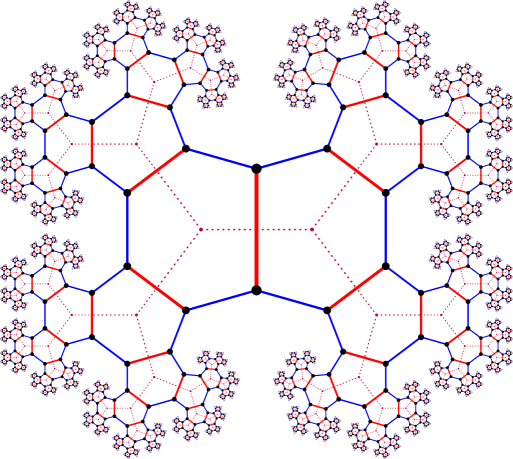
Every element belong to two different hexagons and has exactly one neighbor (predecessor or successor) in each one of these different hexagons (corresponding to the -edges, for and ). We call these neigbors, the -neighbors. Similarly, every element has exactly one neighbor sharing the same two hexagons (corresponding to the -edge), called -neighbor.
On the other hand, each hexagon has a unique vertex of minimal length. Thus, for a given , we can find a vertex of minimal length, sharing a hexagon. We say that the position of is its distance to , that is, .
The cone type of an element is then determined by its position and the combinatorics of the -neighbor being a predecessor or a successor. Note that, whether the -neighbor is a predecessor or a successor is equivalent to consider the position of a point in the unique adjacent -cycle determined by .
The cone type —as in Theorem 3.3— corresponds to the following combinatorics:
-
(0)
The position is and, in particular, the -neighbor is a successor;
-
(1)
The position is and the -neighbor is a predecessor;
-
(2)
The position is and the -neighbor is a successor;
-
(3)
The position is and the -neighbor is a predecessor;
-
(4)
The position is and the -neighbor is a successor; and
-
(5)
The position is and, in particular, the -neighbor is a predecessor.
Reciprocally, this geometric description of the cone types can also be recovered from the combinatorial description given by the -types as follows. The position of is determined by the maximal length of an element in and whether or not there is that ends in the letter , determines whether the -neighbor is a predecessor or a successor, respectively.
3.2. Growth
In this section we follow Cannon’s ideas [Cannon] to compute the growth of relative to .
Proof of Theorem 1.3.
Let be the generating function for the spherical growth sequence , . If is the generating function for the spherical growth sequence of elements of type , that is, of the sequence , .
Now, Theorem 3.3 (cf. Figure 2(a)) implies that there is the following recurrence relation (cf. [Cannon, Proof of Theorem 7]):
and, clearly, .
It follows that the corresponding generating functions satisfy the equations
and .
Finally, solving the recurrence, we get that
and
The growth rate is the reciprocal of radius of convergence of around the origin, which is the root of smallest absolute value of . That is, it is the golden ratio
4. Spectral radius
4.1. Nagnibeda’s ideas for the upper bound
In order to give upper bounds for the spectral radius , we follow Nagnibeda’s ideas [Nagnibeda], which are based in the following elementary result (cf. [ColinDeVerdiere, Chapter II, Section 7.1]) and [Nagnibeda, Section 1]).
Lemma 4.1 (Gabber–Galil).
Let be a finitely generated group and a finite system of generators of . Suppose there exists a function such that, for every and ,
for some . Then, .
Proof.
Since
we get that
Summing over and averaging over , we get
That is, . ∎
For any type function and positive valuation , we can consider a function defined by
Then, every such satisfies , since if and only if .
Aditionally, for , , we define
This is well defined since is a type function and therefore the sum depends only on the type . Note that in the case where every relator has even length, we have that , for every .
As a direct consequence of Gabber–Galil’s Lemma 4.1, we get the following (cf. [Nagnibeda, Section 2]).
Theorem 4.2 (Nagnibeda).
Let be a finitely generated group and a finite system of generators of . Let be a compatible type function for . Then,
for every , where is defined as above. ∎
Then, every type function gives upper bounds for the spectral radius.
Theorem 4.3 (Upper bound for the spectral radius).
Let and . Then, the spectral radius of the random walk on relative to satisfies
Proof.
By Theorem 3.3, the ’s of Nagnibeda’s Theorem 4.2 are given by:
It follows that , for every . Thus, the problem can be reduced to find the optimal such bound. This can be solved numerically: we get that with
is a (local) minimun for , and .
Finally, since , by Nagnibeda’s Theorem 4.2, it follows that
Remark 4.4.
The nature of Nagnibeda’s estimates suggest that it is not possible to improve the upper bound using other type functions. In fact, as shown by Nagnibeda [Nagnibeda:unbeatable, Section 3], these upper bounds correspond to the spectral radius of a random walk on the tree of geodesics of the group and, in particular, do not depend on the choice of the type function. Additionally, it is also shown in [Nagnibeda:unbeatable] that it is possible to compute this upper bound through a recurrence. However, we refrain from doing so here as the resulting estimates are the same (cf. [Nagnibeda:unbeatable, Remark 3.3] ).
4.2. Gouëzel’s ideas for the lower bound
In order to give lower bounds for the spectral radius , we follow Gouëzel’s ideas [Gouezel]. The key tools are essentially the same type functions, but Gouëzel’s techniques allows to neglect a finite number of elements of any type.
More precisely, following [Gouezel, Definition 1.2], we say that is a type system for if it is surjective, is finite and there is such that, for all and all but finitely many with , we have
Then, Gouëzel’s main result to estimate the spectral radius, [Gouezel, Theorem 1.4], reads as follows.
Theorem 4.5 (Gouëzel).
Let be a group, finitely generated by , without relators of odd length. Let be a type system for and suppose that the associated matrix is Perron–Frobenius.
Define the matrix by , where is the number of predecessors of an element of type , that is, . It follows that is also Perron–Frobenius and let be its dominating eigenvalue, which is simple, and let , an associated eigenvector with positive entries.
Let , and . Finally, let be the maximal eigenvalue of the symmetric matrix . Then,
Theorem 4.6 (Lower bound for the spectral radius).
Let and . Then, the spectral radius of the random walk on relative to satisfies
Proof.
Using the type function of Theorem 3.3, by discarding all type and type elements, that is, and , respectively, we get a type system with Perron-Frobenius matrices and , where
Following Gouëzel’s Theorem 4.5, we compute the dominating eigenvalue and corresponding positive eigenvector of , which are
Then, we get , and
Finally, we compute numerically the dominant eigenvalue of the symmetric matrix , which is . Thus, by Gouëzel’s Theorem 4.5, we get that
Note that this is not precisely the estimate from below given in Theorem 1.5. We present it, however to exhibit the computations in detail in a simpler case. We conclude the proof of Theorem 1.5 in LABEL:sect:suffix-type and LABEL:sect:my-type, where we exhibit finer type systems and give the corresponding numerical lower bounds using Gouëzel’s Theorem 4.5.
5. Entropy and drift
In addition to the spectral radius, other important numerical quantities have been introduced to describe the asymptotic behavior of random walks on groups. In this section we estimate some of the most relevant asymptotic invariants: the (asymptotic) entropy and the drift of the random walk. These are defined by
where is the uniform distribution on and , its -fold convolution. Gouëzel, Mathéus and Maucourant [Gouezel-Matheus-Maucourant] showed that estimates on these numerical quantities can be obtained from the others in several ways. More precisely, consider the strictly increasing function defined by
Then, for any (simple, symmetric) random walk on a group, they proved the following (cf. [Gouezel-Matheus-Maucourant, Theorem 1.1]).
Theorem 5.1 (Gouëzel–Matheus–Maucourant).
We have that and .
Previously, Guivarc’h [Guivarch] proved the so-called fundamental inequality between the entropy , the drift and the growth .
Theorem 5.2 (Guivarc’h).
We have that .
Proof of Theorem 1.9.
By Gouëzel–Matheus–Maucourant’s Theorem 5.1, and, by Theorem 1.5, . It follows that
We also have that . Since is increasing in , we have that
On the other hand, , by Theorem 1.3. Thus, by Guivarc’h’s Theorem 5.2, we get
Appendix A The modular group as a free product of cyclic groups. A brief survey
In this appendix, we include a brief survey on analogous results in the case of the generating system , where and . Note that, one has , for .
With this generating system, we have the presentation . In particular, as abstract group, is the free product of the cyclic groups of order two and three, that is, and the elements in correspond to generators for the cyclic groups (see, e.g., [Alperin]).
The Cayley graph of such a free product relative to the cyclic generators has a particularly easy structure and a much more detailed descriptions of the objects studied in this work is possible. For example, one can easily derive the growth series. In fact, it is enough to count the reduced words in with no repeated consecutive letters. A recurrence can then be easily derived by counting such words that end with an separately from those ending in or .
Theorem A.1 (Growth).
Let and . Then, the growth series of relative to corresponds to the rational analytic function
In particular, the rate of exponential growth of relative to is
This is not different in essence from what we do for the generating system in Section 3. However, in this case, the simpler structure allows an easier understanding of the combinatorics. In fact, geodesics words are exactly the reduced words with no consecutive occurrences of letters, and the ending letter of such a geodesic determines the cone type of the corresponding group element.
Theorem A.2 (Cone types).
Let and . Then, there are exactly three cone types: , and . ∎
With considerably more work, it is also possible to describe completely the spectrum of the simple symmetric random walk on associated with (see [Gutkin, Theorem 4]; originally proved in [McLaughlin]).
Theorem A.3 (Markov spectrum).
Let and . And consider the Markov operator associated with the simple symmetric random walk on relative to . Then, the point spectrum of is and the absolutely continuous spectrum of is
In particular, the spectral radius of the random walk on relative to is
Corollary A.4 (Laplace spectrum).
Let and . And consider the combinatorial Laplace operator on relative to . Then, the point spectrum of is and the absolutely continuous spectrum of is
In particular, the bottom of the spectrum of the Laplace operator on relative to is
Furthermore, it is also possible to compute the other asymptotic invariants of a random walks on a free product of cyclic groups (see [Mairesse-Matheus, Sections 4.2 and 5.1]).
Theorem A.5 (Asymptotic invariants).
Let and . Then, the rate of exponential growth , the entropy and the drift satisfy . Moreover,
Cayley graph
In the case of and , the Cayley graph has a minor regular tree of degree three, where each vertex in correspond to a triangle (-cycles) in and the edges of correspond to the -edges of . See Figure 4 for a representation of the (undirected colored) Cayley graph . Each red -edge corresponds in fact to the -cycle given by the relator and the triangles, to the primitive relators of length three: and .
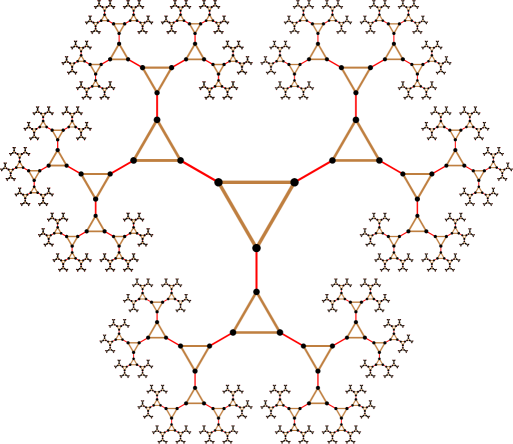
In particular, every element belong to exactly one triangle and every triangle contains a single vertex of minimal length, determining the cone type of any element other than the identity. In fact, an element is of minimal length in its triangle if and only if its only geodesic ends with the letter .
Appendix B Another geometrically meaningful generating system
In this appendix, we include a summary of the analogous results in the case of the generating system , where and . Note that , where .
In this case, we have the presentation and the set of primitive relators is
Theorem B.1 (Cone types).
Let and . Then, there are exactly three cone types for relative to : , and .
Proof.
Since all primitive relators are of length at most four, any suffix of a geodesic that is a subword of a primitive relator has length at most two. It follows that the type function from Proposition 2.5 can only take values in the set
and any such value is possible. In LABEL:tab:diagram-2, we describe the -type of their successors. Such description follows easily from the definition of and the description of the primitive relators above. We also include the types of the neighbors of the same length. This is needed as there are relators of odd length (see Remark 2.3).
Now, it is clear also from the primitive relators that the involution that interchange each letter in with its inverse, defines an automorphism of the corresponding Cayley graph and, in particular, isomorphisms between the respective cones. Thus, we have , , and .
Moreover, it is still possible to reduce the number of cone types noticing that . For simplicity, let be defined as follows:
Then, by the description of the -types in LABEL:tab:diagram-2, it is clear that is a type function. In particular, determines the cone types (see also LABEL:fig:cone-types-2).
It only remains to prove that different -types define different cone types. But this follows easily, similarly as in the proof of Theorem 3.3, simply counting the number of elements in the level one in each rooted graph (see LABEL:fig:different-cone-types-2). ∎
| E(g) | E(gs):s∈S”_+(g) |
| ∅ | {t}, {¯t}, {u}, {¯u} |
| {t} | {t¯u, u¯t}, {u} |
| {¯t} | {¯tu, ¯ut}, { |