Towards Highly Accurate Coral Texture Images Classification Using Deep Convolutional Neural Networks and Data Augmentation

Abstract

The recognition of coral species based on underwater texture images pose a significant difficulty for machine learning algorithms, due to the three following challenges embedded in the nature of this data: 1) datasets do not include information about the global structure of the coral; 2) several species of coral have very similar characteristics; and 3) defining the spatial borders between classes is difficult as many corals tend to appear together in groups. For this reason, the classification of coral species has always required an aid from a domain expert. The objective of this paper is to develop an accurate classification model for coral texture images. Current datasets contain a large number of imbalanced classes, while the images are subject to inter-class variation. We have analyzed 1) several Convolutional Neural Network (CNN) architectures, 2) data augmentation techniques and 3) transfer learning. We have achieved the state-of-the art accuracies using different variations of ResNet on the two current coral texture datasets, EILAT and RSMAS.

1 Introduction

Coral reefs are complex marine ecosystems typical to the warm and shallow seas of the tropics. The reefs are created by the slow accumulation of hard calcium carbonate skeletons that hard coral species leave behind when they die, waiting for another coral to live in it and expand the reef. Coral reefs are one of the most valuable ecosystems in the world as they are extremely biodiverse. They support up to two million species and a quarter of all marine life on Earth [ESI, 2017]. They are also very important from the human point of view [Ferrario et al., 2014]. Coral species help to clean the water and remove nitrogen and carbon, they are a source for medicine research and economic wealth from fishing and tourism, they are also a natural barrier for coastal protection against hurricanes and storms and, since many of them are thousands and even millions years old, their study helps scientists to understand climatic events of the past.

The study of the distribution of coral reefs over time can provide important clues about the impact of global warming and water pollution levels. According to ESI [2017], we have already lost 19% coral reefs areas since the 1950s and, according to the International Union for Conservation of Nature (IUCN) Red List of Threatened Species [IUCN, 2017], in 2017 there were 237 threatened species in the evaluated 40% of the estimated total of species. This is due to the fact that coral reefs do not tolerate temperature changes and a quarter of the carbon dioxide emissions in the atmosphere is absorbed by the ocean, in addition to the water pollution and other problems caused by humans.

With recent advancements in image acquisition technologies and growing interest in this topic among the scientific community, huge amount of data on coral reefs is being collected. However, it is complicated to keep a record of all coral species because there are thousands of them and the taxonomy is mutable. This is due to new discoveries made by scientist or because they may change the order, family or genus of existing species as they gather more knowledge about them. In addition, some coral species have different sizes, shapes and colors, but other coral species seem to be identical for a human observer. As a consequence, a successful coral classification has always demanded an expert biologist. If we can automate the classification by using the amount of coral images that is being collected, we can help scientists to study more closely that amount of data, making an important step towards automatic knowledge discovery process. In fact, automatizing the classification process of coral images has been addressed in a few number of works. Most of them [Beijbom et al., 2012, Pizarro et al., 2008, Shihavuddin et al., 2013, Stokes & Deane, 2009] use machine learning models combined, in some cases, with image enhancement techniques and feature extractors. Among these works, only Shihavuddin et al. [2013] use several datasets.

In recent years, Convolutional Neural Networks (CNNs) have shown outstanding accuracies for image classification [Krizhevsky et al., 2012, Russakovsky et al., 2015], especially in the field of Computer Vision. Currently, their applications branch out to a plethora of diverse fields, where analysis of image data is required. In biology, CNNs have been evaluated and compared with machine learning algorithms for wood classification [Affonso et al., 2017]. In coral classification, the use of CNNs is challenging due to the variance between images of the same class, the lightning variations due to the water column or the fact that some coral species tend to appear together. Besides, CNNs need a large dataset to achieve a good performance. In practice, two techniques are used to overcome this limitation: transfer learning and data augmentation. There are some works that use CNNs for coral classification [Elawady, 2015, Mahmood et al., 2016a, b], but they use popular CNNs, like VGGnet or LeNet and they only use one dataset to test their models. Besides, they not use EILAT or RSMAS.

We propose to use more capable CNNs to overcome the limitations of previously applied deep learning models. We want to develop a much more accurate model approaching the human expert, facing the specific problems of coral classification using several datasets. In particular, we have considered three of the most promising CNNs, Inception v3 [Szegedy et al., 2016], ResNet [He et al., 2016] and DenseNet [Huang et al., 2017]. Inception is a newer version of GoogleNet, which won the ImageNet Large Scale Visual Recognition Competition (ISLVRC) [Russakovsky et al., 2015] competition in 2014. ResNet won the same competition in 2015 and DenseNet beat the results of ResNet in 2016. We have considered two underwater coral datasets, RSMAS and EILAT [Shihavuddin, 2017], and we have compared our results with the most accurate model [Shihavuddin et al., 2013]. In these datasets, the images are patches of the corals, that is, they are small and they show a little part of the coral, a texture, not the entire structure of the coral.

The contributions of this work are the following:

• Study, explore and analyze the performance of the most promising CNNs in the classification of underwater coral texture images.

• Analyze the impact of data augmentation on the performance of the coral texture classification model.

• Compare our results with the state-of-the-art classical methods which require high human supervision and intervention.

The rest of the paper is organized as follows. An overview of the three considered CNNs is provided in Section 2. The challenges of coral classification and related works are given in Section 3. A description of the coral datasets we have used is provided in Section 4. The experiments and results are given in Section 5 and the final conclusions of this study are given in Section 6.

2 CNN Classification Models

CNNs have achieved outstanding accuracies in a plethora of contemporary applications, automatizing its design [Ferreira et al., 2018]. In fact, since 2012 the prestigious ILSVRC competition [Russakovsky et al., 2015] have been won exclusively by CNN models. The CNN layers capture increasingly complex features as the depth increases. In recent years, these architectures have evolved by increasing first the depth of the networks, then the width and finally using lower features obtained from the lower layers into higher layers. This section provides an overview of the CNNs used in this work. We have considered three influential CNNs, Inception v3 (Subsection 2.1), ResNet (Subsection 2.2), and one of the newest, DenseNet, (Subsection 2.3). Finally, we describe the optimization techniques that we have used to overcome the small sizes of the considered datasets (Subsection 2.4).

2.1 Inception v3

GoogLeNet [Szegedy et al., 2015] won the ILSVRC in 2014 and it is based on the repetition of a module called inception. This module have six convolutions and one max-pooling. Four of these convolutions use a 1$\times$1 kernel, which is introduced to increase the width and the depth of the network and to reduce the dimensionality when it is necessary. In this sense, a $1\times 1$ convolution is performed before the other two convolutions in the module, a $3\times 3$ and a $5\times 5$ convolution. After all the computation, the output of the module is calculated as the concatenation of the output of the convolutions. This module is repeated 9 times and at the end it uses a dropout layer. In total, GoogLeNet has 22 learnable layers.

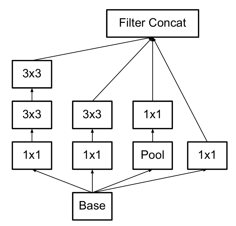
Figure 1: Base Inception v3 module. Figure from [Szegedy et al., 2016].

Inception v3 can be considered as a modification of GoogLeNet. The base inception module is changed by removing the $5\times 5$ convolution and introducing instead two $3\times 3$ convolutions, as we can see in Figure 1. The resulting network is made up of 10 inception modules. Furthermore, the base module is modified as the network goes deeper. Five modules are changed by replacing the $n\times n$ convolutions by a $1\times 7$ followed by a $7\times 1$ convolution in order to reduce the computational cost. The last two modules replace the last two $3\times 3$ convolutions by a $1\times 3$ and a $3\times 1$ convolutions each one, this time in parallel. Lastly, the first $7\times 7$ convolution in GoogLeNet is also changed by three $3\times 3$ convolutions. In total, Inception v3 has 42 learnable layers.

2.2 ResNet

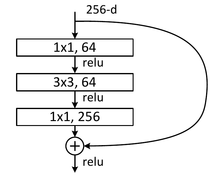
Figure 2: ResNet building block. Figure from [He et al., 2016].

Increasing the network depth to obtain a better precision makes the network more difficult to optimize since it may produce the vanishing or exploding gradients problem. ResNet [He et al., 2016], which won the ILSVRC classification task in 2015, address this issue by fitting a residual mapping instead of the original mapping, and by adding several connections between layers. These new connections skip various layers and perform an identity, which not adds any new parameters, or a simple $1\times 1$ convolution. In particular, this network is also based on the reiterated use of a module, called a building block. The depth of the network depends on the number of the used building blocks. For 50 or more layers, the building block consists of three convolutions, a $1\times 1$ followed by a $3\times 3$ followed by a $1\times 1$ convolution, and a connection joining the input of the first convolution to the output of the third convolution, as we can see in Figure 2. For our problem, we have used the model with 50 layers, ResNet-50, and with 152 layers, ResNet-152.

2.3 DenseNet

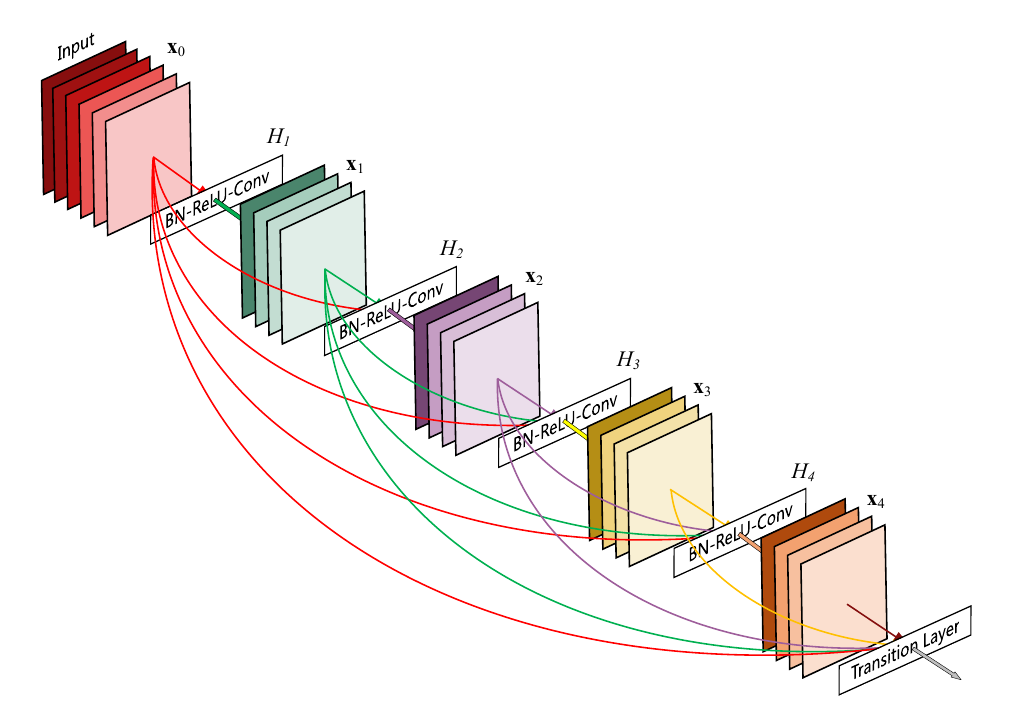
Figure 3: Example of a dense block. Figure from [Huang et al., 2017].

DenseNet is also based on the repetition of a block, called the dense block. Inspired by the building block of ResNet, DenseNet connects the output of all the layers to the input of all the following layers within the dense block [Huang et al., 2017]. The connections between blocks, called transition layers, work as a compression factor in a sense that the transition layer generates less feature maps than it receives. The difference between connections in the dense block and connections in the building block of ResNet is that in the dense block the outputs of previous layers are added to the following layers before its computation is performed. A dense block is the repetition of a Batch Normalization, a ReLU, a $1\times 1$ convolution, a Batch Normalization, a ReLU and a $3\times 3$ convolution a specific number of times. In Figure 3 we can see an example of a DenseNet block. The transition layers are a $1\times 1$ convolution followed by an average pool with kernel $2\times 2$. Similarly to ResNet, the number of dense blocks determines the number of layers in the network. In this work, we have analyze DenseNet-121 and DenseNet-161, which include 121 and 161 layers respectively.

2.4 CNN Optimization Techniques

CNN-based models require a large set of training samples to achieve good generalization capabilities. However, generating large datasets is either costly, time-consuming, or sometimes simply impossible. In practice, two techniques are used to overcome this limitation: transfer learning and data augmentation. Since the current coral datasets are too small to train an effective CNN from scratch, we propose to use these two approaches:

• Transfer learning: instead of starting the training from a scratch by randomly initializing weights, we initialize weights using a pre-trained network on different datasets, usually much larger in size. In this work, we have considered using the knowledge learned from ImageNet [Deng et al., 2009] in our coral classification. We remove the layer that classifies the images into the classes of ImageNet and we add two fully connected layers that classify the images into our concrete problem. We train these last two layers, instead of fine-tune the whole network, which would also require larger datasets.

• Data augmentation: consists of artificially increasing the volume of the training set by applying several distortions to the original images, such as changing the brightness, scaling or zooming, rotation, vertical or horizontal mirroring, etc. The applied distortions should not alter the spatial pattern of target classes [Tabik et al., 2017]. Usually the distortions are performed during the training time, which allows to do it on the fly without saving the new images.

3 Previous Advances on Automatic Coral Reef Classification

In this section we explain the challenges of the underwater coral and coral reef images classification and we give an overview on existing works for automating the classification of coral reef habitat using underwater imagery. The reasons why the classification of such images is difficult are provided in Subsection 3.1. Previous works in coral classification can be divided into two groups, methods that combine classical models (Subsection 3.2) and methods that use CNNs (Subsection 3.3).

3.1 Challenges of Coral Classification

The classification of underwater coral images is challenging for the following reasons:

• Partial occlusion of objects due to the three-dimensional structure of the seabed. Depending on the water type, there can be significant variation in presence of scattering effect, which increases additive noise on the image acquisition and makes it difficult for any computer vision algorithm to perform as in a normal environment.

• Lightning variations due to wave focusing and variable optical properties of the water column. In the deep underwater scenario, it is common that there is no natural light source other than the remote sensing device, which implies non uniform illumination across the acquired images.

• Subjective annotation of the training samples by different analysts.

• Variation in viewpoints, distances and image quality.

• Significant inner-class variability in the morphology of benthic organisms.

• Complex spatial borders between classes, as many coral species tend to appear together.

• The difficulty of keeping the autonomous vehicles stable in the underwater environment, which creates significant motion blur when the images are acquired in a video format.

• There are very few datasets of underwater coral reef images and in general they contain patches of the texture of the coral, while at the same time they do not include any information on the global structure of the coral.

3.2 Coral Classification Based on Classical Methods

Most of the existing approaches for classifying underwater coral images combine one feature extractor with a classifier and show their performance only using a single dataset, i.e., with specific size, resolution of the images, number of classes and color information [Beijbom et al., 2012, Pizarro et al., 2008, Stokes & Deane, 2009]. The first paper in this subject was by Pizarro et al. [2008]. The authors analyze more marine habitat besides corals, so it is more general. They use a SIFT descriptor and a bag of features approach, which means that they choose from the training set the images that are more similar to each test image. Beijbom et al. [2012] introduced the Moorea Labelled Corals (MLC) dataset, which has large images containing different coral species, and they used Support Vector Machines along with filters and a texture descriptor. They obtained an accuracy of 83.1% on this dataset using the images of 2008 and 2009 for training and the images of 2010 for testing. Stokes & Deane [2009] used a normalized color space and a discrete cosine transform to extract texture features. Again, they only used one dataset, provided by the National Oceanic and Atmospheric Administration (NOAA) of the U.S. Department of Commerce Ocean Explorer.

The portability of these methods to new datasets has not been demonstrated yet. Only Shihavuddin et al. [2013] developed an unified classification algorithm for four different datasets of different characteristics, in which we can find RSMAS and EILAT. The authors combined multiple image enhancement techniques, feature extractors and classifiers, among other techniques. In particular, the image enhancement step contain four algorithms, one mandatory (Contract Limited Adaptive Histogram Specification or CLAHS) and three optional (color correction, normalization and color channel stretching). The feature extraction step contain one optional, used as color descriptor, and three mandatory algorithms, used as texture descriptors. Then, the method has a kernel mapping step with three mandatory algorithms, a dimension reduction step with two optional algorithms and a prior settings step with one algorithm. Then it performs the classification using one of the following algorithms: SVM multiclass, KNN, a neural network or probability density weighted mean distance. Lastly, if the original image was a mosaic containing several patches, it uses a thematic mapping using sliding window and morphological filtering. By configuring the hyperparameters and the different combinations of these algorithms, the model can be adapted to different datasets.

This method is considered to be the state-of-the-art for RSMAS and EILAT datasets. In particular, in these two datasets the best combination of algorithms is the following: in the image enhancement step it uses just CLASH. In the feature extraction step it uses the opponent angle histogram, the hue channel histogram, the grey level co-occurrence matrix, the completed local binary pattern and the Gabor filter response. In the kernel mapping step it uses L1 normalization, chi-square kernel and Hellinger kerl for the completed local binary pattern and the color histogram. In the dimension reduction step it uses principal component analysis and Fisher kernel. In the prior settings step it uses class frequency to estimate prior probability. Finally, as classification algorithm it uses KNN.

As it can be seen, this algorithm implies a lot of human supervision and intervention, as there we need to test a lot of algorithms with several hyperparameters and many possible combinations between the algorithms. Furthermore, when we have the best combination we need to use a lot of algorithms every time we need to classify a new image. In the particular case of EILAT and RSMAS, we need to use six algorithms to obtain the classifier and every time we need to classify a new image we need to use the first four algorithms, until we obtain the features of the image.

3.3 Coral Classification Based on CNNs Methods

The use of CNNs for coral classification allow us to use the images without the image enhancements, although it is possible to use them, and without the feature extraction, saving a lot of experiments to detect the best combination of algorithms and therefore, saving time.

The first work that used CNNs for coral classification was by Elawady [2015]. The authors first enhanced the input raw images via color correction and smoothing filtering. Then, they trained a LeNet-5 [LeCun et al., 1998] based model whose input layer consisted of three basic channels of color image plus extra channels for texture and shape descriptors consisting of the following components: zero component analysis whitening, phase congruency, and Weber local descriptor. The model obtained around 55% accuracy on the two datasets they used.

Mahmood et al. [2016a] use VGGnet [Simonyan & Zisserman, 2014] pretrained on ImageNet and the dataset BENTHOZ-2015 [Bewley et al., 2015] to fine-tune the network. This dataset contains more than 400,000 images and associated sensor data collected by an autonomous vehicle over Australia. The authors extract several patches from each image centered in different pixels and using different scales and they apply a color channel stretch to the patches as a pre-processing technique. In this article, they propose a mechanism to automatically label unseen coral reef images to obtain the coral coverage in the region where the images are collected (i.e., classifying new images as coral or non-coral ones). A marine expert later verifies the accuracy of this automatic method. In the presented experimental study, authors conducted several experiments and reported over 90% accuracy obtained in each of them.

Mahmood et al. [2016b] use the MLC dataset to propose the usage of CNNs along with hand-crafted features. Moreover, they introduce a mechanism to extract such features. This proposal is based on the observation that CNNs cannot be trained from scratch using the available coral datasets due to its small size. The features extraction with CNNs has been carried out with the network VGGnet pre-trained on ImageNet. To classify both types of features, they use a two layer Perceptron. In their experiments, they obtain better accuracies with this technique than just with VGGnet or just the hand-crafted features, although the difference between VGGnet and the combination of the features is small. In their best experiment, they obtain an accuracy of 84.5% in MLC.

These works use classical CNNs: VGGnet and LeNet and they do not use EILAT or RSMAS. Besides, sometimes the accuracies obtained are low [Elawady, 2015], the classification is simple [Mahmood et al., 2016a] or they use hand-made feature extraction along with CNNs [Mahmood et al., 2016b].

4 Datasets

There exist eight open benchmarks used for underwater coral classification. These include five public color datasets: EILAT, RSMAS, MLC, EILAT2 (a subset of EILAT) and the Red Sea Mosaic dataset. The remaining three are black and white datasets: UIUCtex, CURET and KTH-TIPS. Some of them include non-coral classes such as fabric, wood and brick. It is worth to mention that the Red Sea Mosaic dataset is actually one single large image that contains a large number of different coral species.

In this work, we have used the most recent RGB datasets that contain the highest number of corals, RSMAS and EILAT [Shihavuddin, 2017]. These two datasets are comprised of patches of coral images. These patches capture mainly the texture of different parts of the coral and do not include any information of the global structure of the entire coral. The usage of CNNs with texture images has already been successfully carried out for granite tiles classification [Ferreira & Giraldi, 2017]. In this case, both datasets are also highly imbalanced. Some classes have a high number of samples whereas other classes include very few samples, which makes the classification more difficult. The main characteristics of these two datasets are as follows:

• EILAT contains 1123 image patches of size $64\times 64$, taken from coral reefs near Eilat in the Red sea. The image patches are pieces of larger images. The original images were taken under equal conditions and with the same camera. See examples of patches in Figure 4. The patches have been classified into eight classes, but the used labels do not correspond to the coral species names. EILAT is characterized by imbalanced distribution of examples among classes, as it can be seen in Table 1.

• RSMAS contains 766 image patches of size 256$\times$256. The images were collected by divers from the Rosenstiel School of Marine and Atmospheric Sciences of the University of Miami. These images were taken under different conditions as they were taken with different cameras in different places. See examples in Figure 5. The patches have been classified into 14 classes, whose labels correspond to the names of the coral species in Latin, as it can be seen in Table 1.

5.4cm][b].2

(a) Sand

5.4cm][b].2

(b) Urchin

5.4cm][b].2

(c) BranchesI

5.4cm][b].2

(d) Brain Coral

5.4cm][b].2

(e) Favid Coral

5.4cm][b].2

(f) BranchesII

5.4cm][b].2

(g) Dead Coral

5.4cm][b].2

(h) BranchesIII

Figure 4: Selected patches from EILAT. Each column shows two examples per class.

4.4cm][b].15

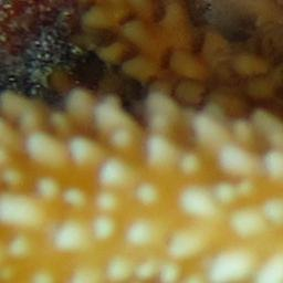
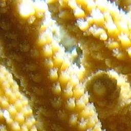
(a) ACER

4.4cm][b].15

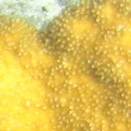
(b) APAL

4.4cm][b].15

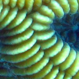
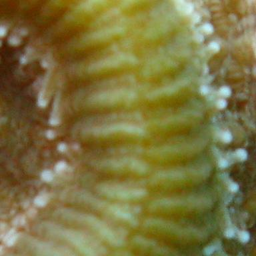
(c) CNAT

4.4cm][b].15

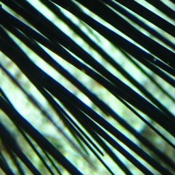
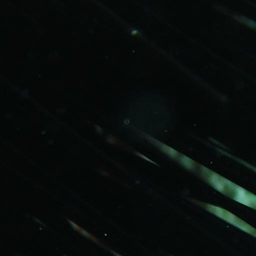
(d) DANT

4.4cm][b].15

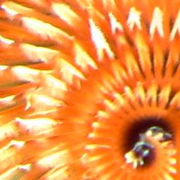
(e) DSTR

4.4cm][b].15

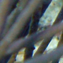
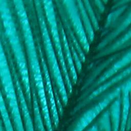
(f) GORG

4.4cm][b].15

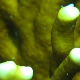
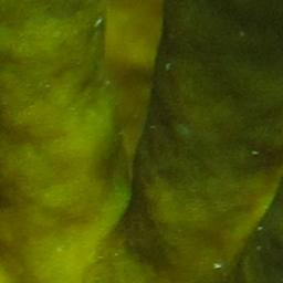
(g) MALC

4.4cm][b].15

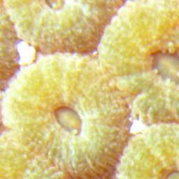
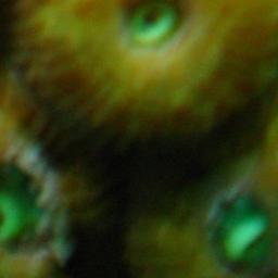
(h) MCAV

4.4cm][b].15

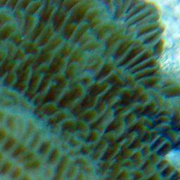
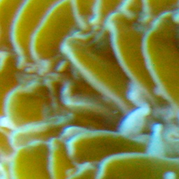
(i) MMEA

4.4cm][b].15

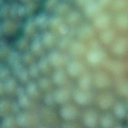
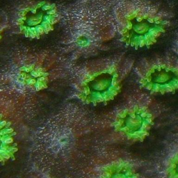
(j) MONT

4.4cm][b].15

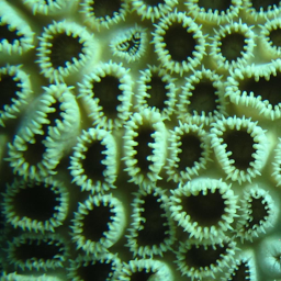
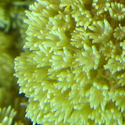
(k) PALY

4.4cm][b].15

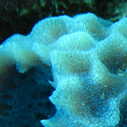
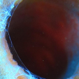
(l) SPO

4.4cm][b].15

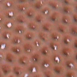
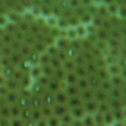
(m) SSID

4.4cm][b].15

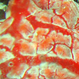
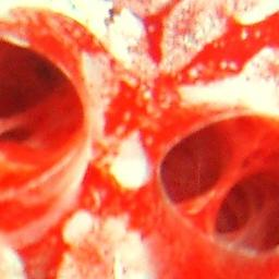
(n) TUNI

Figure 5: Selected patches from RSMAS. Each column shows two examples per class.

Table 1: Characteristics of EILAT, RSMAS and StructureRSMAS. The #imgs refers to the number of images in the corresponding class.

Dataset	Classes	#imgs
EILAT	Sand.	$87$
	Urchin.	$78$
	Branches Type I.	$29$
	Brain Coral.	$160$
	Favid Coral.	$200$
	Branches Type II.	$216$
	Dead Coral.	$296$
	Branches Type III.	$11$
RSMAS	Acropora Cervicornis (ACER).	$109$
	Acropora Palmata (APAL).	$77$
	Colpophyllia Natans (CNAT).	$57$
	Diadema Antillarum (DANT).	$63$
	Diploria Strigosa (DSTR).	$24$
	Gorgonians (GORG).	$60$
	Millepora Alcicornis (MALC).	$22$
	Montastraea Cavernosa (MCAV).	$79$
	Meandrina Meandrites (MMEA).	$54$
	Montipora spp. (MONT).	$28$
	Palythoas Palythoa (PALY).	$32$
	Sponge Fungus (SPO).	$88$
	Siderastrea Siderea (SSID).	$37$
	Tunicates (TUNI).	$36$

5 Classification of Coral Texture Images with CNNs

This section is organized in four parts. First, we describe the experimental framework we have used (Subsection 5.1). Second, we analyze the results of our CNN-based classifiers without data augmentation and compare them with the state-of-the-art classical models on EILAT and RSMAS (Subsection 5.2). Third, we analyze the impact of data augmentation on these two texture datasets (Subsection 5.3). Finally, we provide a deeper analysis on the missclassified EILAT and RSMAS images by their best models (Subsection 5.4).

5.1 Experimental Framework

All the results provided in this section have been obtained performing a 5 fold cross validation technique. To analyze and compare the performance of different CNNs architectures, configurations and optimizations, we have used the mean of the five accuracies obtained in the five folds. The accuracy is calculated as follows:

$$\mathrm{Accuracy}=\frac{\mathrm{True\ Positives}+\mathrm{True\ Negatives}}{N}\enspace,$$

where $N$ is the total number of instances.

To evaluate ResNet and DenseNet, we have used Keras [Chollet et al., 2015] as front-end and Tensorflow [Abadi et al., 2015] as back-end. To evaluate Inception, we have used its implementation in Tensorflow. We have used transfer learning by initializing the considered CNNs with the pre-trained weights of the networks on Imagenet. We have also analyzed the impact of these data augmentation techniques on the performance of the learning process:

• Random shift (referred to later as shift) consists of randomly shifting the images horizontally or vertically by a factor calculated as the fraction of the width or length of the image. In this work we shift the images horizontally and vertically in all the cases. Given a number $x$, the width and length of the image will be shifted by a random factor selected in the interval $[0,x]$.

• Random zoom (referred to later as zoom) consists of randomly zooming the image by a certain range. Given a value $x$, each image will be resized in the interval $[1-x,1+x]$.

• Random rotation (referred to later as rotation) consist of randomly rotating the images by a certain angle. Given a value $x$, each image will be rotated by an angle in $[0,x]$.

• Random horizontal flip (referred to later as flip) consist of randomly flipping the images horizontally.

3.8cm][b].3

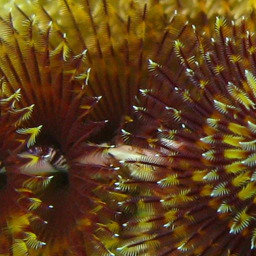
(a) Original

3.8cm][b].3

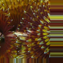
(b) Shift

3.8cm][b].3

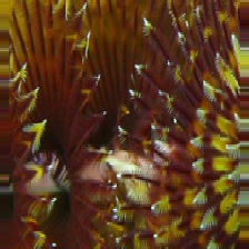
(c) Zoom

3.8cm][b].3

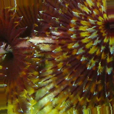
(d) Rotation

3.8cm][b].3

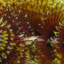
(e) Flip

Figure 6: The result of applying four data augmentation techiques to (a) a original RSMAS image: (b) shift, (c) zoom, (d) rotation and (e) flip.

An illustration of these data augmentation techniques is shown in Figure 6. As it can be seen, the distorted images maintain the original size and the pixels outside the boundaries are filled with the values of the limit pixels. This effect can be clearly seen in Figure 6(b).

Besides these data augmentation techniques, we have also evaluated the impact of different hyperparameters on the performance of the analyzed networks, such as the number of iterations, the batch size and the number of layers.

5.2 Classification of Coral Texture Images without Data Augmentation

Table 2: The accuracies obtained by Inception v3, ResNet-50, ResNet-152, DenseNet-121, DenseNet-161 and the classical state-of-the-art Shihavuddin model. The results of all the Convolutional Neural Networks (CNNs) were obtained without data augmentation. The best results are stressed in bold.

	Shihavuddin’s method	Inception v3	ResNet-50	ResNet-152	DenseNet-121	DenseNet-161
EILAT	95.79	95.25	97.85	97.85	91.03	93.81
RSMAS	92.74	96.03	97.67	97.95	89.73	91.10

Table 3: The set of hyperparameters that provides the best performance shown in Table 2 for each CNN model.

		Inception v3	ResNet-50	ResNet-152	DenseNet-121	DenseNet-161
EILAT	Batch Size	100	64	64	32	32
	Epochs	4000	500	300	300	700
RSMAS	Batch Size	100	64	32	32	64
	Epochs	4000	1300	300	700	1000

In this subsection we have evaluated exhaustively Inception v3, ResNet and DenseNet with different hyperparameters and we have compared the results obtained for these three CNNs with the state-of-the-art model by Shihavuddin et al. [2013] on EILAT and RSMAS. For Inception, we have analyzed the impact of different numbers of iterations and batch sizes. For ResNet and DenseNet, we have evaluated different combinations of number of epochs, batches sizes and network depths.

As the results provided by Shihavuddin et al. [2013] were performed using a 10 fold cross validation, we had to re-evaluate their model using a 5 fold cross validation with the same folds we have used for all other models in order to compare them under the same conditions. We have also used the best hyperparameters for each dataset at each step of the method described in Subsection 3.2.

The results of Shihavuddin’s method, Inception v3, ResNet with 50 and 152 layers and DenseNet with 121 and 161 layers are shown in Table 2, while the corresponding best configurations are shown in Table 3. As it can be seen from this table, ResNet-152 outperforms Shihavuddin’s model and the rest of the CNN models. Inception provides a better accuracy than Shihavuddin’s method on RSMAS, but shows a worse accuracy on EILAT. DenseNet shows the worst results on both datasets. In general, these results show that CNNs are able to become the state-of-the-art in coral classification tasks. In RSMAS, the best model is ResNet-152, with more than a 5% improvement with respect to Shihavuddin’s method. In EILAT, ResNet-50 and ResNet-152 achieve exactly the same accuracy, it is not a cause of rounding, and they outperform Shihavuddin’s method for more than 2%.

Obtained results allow us to conclude that only by training the last layers of a CNN that is already pre-trained on ImageNet and without data augmentation, which is the technique that usually takes more time, we can outperform a method that takes long running times and need high human supervision. In fact, Shihavuddin’s method is composed of six steps and each step is composed of one or various algorithms. Then, in order to obtain the best performance, it is needed to evaluate all the possible algorithm combinations through all the steps and to optimize the hyperparameters of each algorithm. Furthermore, this has to be done independently for each dataset we want to classify.

5.3 Classification of Coral Texture Images with Data Augmentation

In this subsection we have analyzed the effect of the data augmentation techniques listed in Subsection 5.1 on the classification of texture images. To carry out this analysis, we have selected the best performing model for each dataset. In EILAT, ResNet-50 and ResNet-152 are the best models and provide the same accuracy, so we have chosen ResNet-50 as it is simpler and has less parameters. In RSMAS, the best model is ResNet-152.

Recall that if we note rotation = 2, it means that we are applying a random rotation to the images by an angle in the interval $[0,2]$. This notation is equivalent for all the other techniques.

Table 4: The accuracies obtained by the best performing CNN on EILAT, ResNet-50, with different data augmentation techniques using the set of hyperparameters indicated in Table 3. The best result is stressed in bold.

	without data augmentation	shift = 0.2	zoom = 0.2	rotation = 2	flip	shift = 0.2, zoom = 0.2
Accuracy	97.85	98.03	97.85	97.40	97.53	97.85

Table 5: The accuracies obtained by the best performing CNN on RSMAS, ResNet-152, with different data augmentation techniques using the set of hyperparameters indicated in Table 3. The best result is stressed in bold.

	without data augmentation	shift = 0.2	zoom = 0.4	rotation = 2	flip	shift = 0.2, zoom = 0.4
Accuracy	97.95	98.36	98.63	97.40	97.578	98.08

Tables 4 and 5 show respectively the results of ResNet-50 and ResNet-152 on EILAT and RSMAS using data augmentation together with the parameters that provide the best performance. The number of steps is the number of times that we generate a batch of new images by data augmentation at each epoch. As the number of steps increases, the accuracy improves but also the time needed to complete each experiment increases. In this case, 300 was the best number of steps. Although we are only showing the best accuracies we have obtained from using data augmentation, the difference in accuracy between the best data augmentation technique and the results obtained without data augmentation is quite small. In both cases the improvement is less than 1%.

This slight improvement using data augmentation can be explained by the nature of used images. Since the original images are small and close-up, the applied modifications do not have much effect on the learning of the models as they need to be small: the shift implies to loose part of the images, and they are already very small; and the zoom implies to loose quality of the images, and they are already blurry because they are underwater images. On the other hand, the images are so close-up that the rotation and the flipping do not introduce significant variations among them. Besides, the performance of the base models is already good without any data augmentation. Therefore, we can conclude that the use of data augmentation techniques in texture coral images does not significantly improve the learning model.

5.4 Analyzing the Missclassified Images

In this subsection we have analyzed the missclassified images in each partition of the 5 fold cross validation in both datasets, EILAT and RSMAS.

2.7cm][b]

(a) Examples of five images missclasified as Dead Coral

2.7cm][b]

(b) Dead Coral images

Figure 7: Examples of (a) missclassified images in EILAT as Dead Coral and (b) original Dead Coral images.

2.7cm][b]

(a) Branches Type III images

2.7cm][b]

(b) Branches Type II images

Figure 8: Examples that show the similarities between (a) Branches Type III and (b) Branches Type II. The third image form (a) is missclasified as Branches Type II. The first and second images from (b) are missclassified as Branches Type III.

In EILAT, ResNet-50 produced 22 missclassified images in all of the test folds. 14 of this missclassified images have been classified as Dead Coral. Dead Coral is the class with the highest number of images as all the dead corals (no matter what species) are in this class. This implies that this class shares some features with all the other classes, as we can see in Figure 7. Additionally, this may also be caused by a classification bias emerging due to the imbalance nature of EILAT [Krawczyk, 2016]. Similarly, there are four Dead Coral images classified as other classes. In total, 18 of 22 images are missclassified due to this class. The remaining three images are from the class Branches Type II missclassified as Branches Type III or vice versa. As we can observe in Figure 8, some images in these two classes are very similar and therefore it is very difficult to distinguish between them.

2.7cm][b]

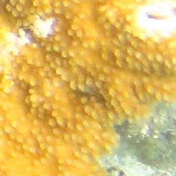
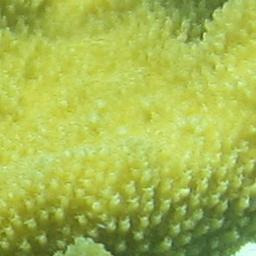
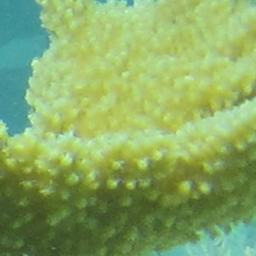
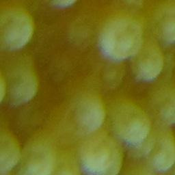
(a) APAL

2.7cm][b]

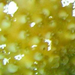
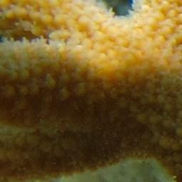
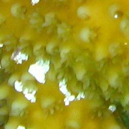
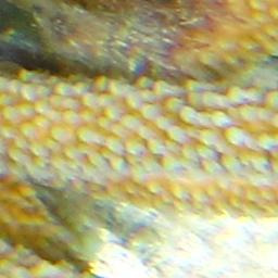
(b) ACER

Figure 9: Examples that show the similarities between (a) APAL and (b) ACER. The third and fourth images from (a) are missclassified as ACER. The first and second images from (b) are missclassified as APAL.

2.7cm][b]

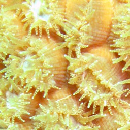
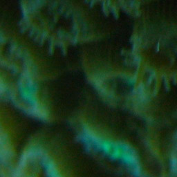
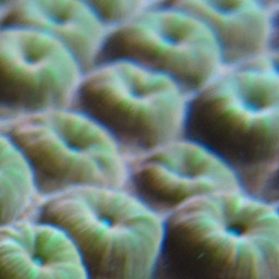
(a) MCAV

2.7cm][b]

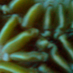
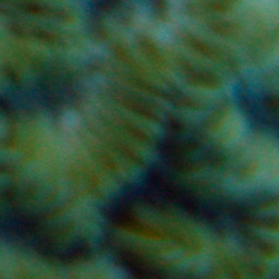
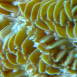
(b) MMEA

Figure 10: Examples that show the similarities between (a) MCAV and (b) MMEA. The second and third images in (a) are missclassified as MMEA.

In RSMAS, ResNet-152 produced only 10 missclassified images in all of the test folds. In general, the model tends to missclassify APAL as ACER and vice versa. The model always missclassified MCAV as MMEA. We can see the similarities between these classes in Figures 9 and 10. The rest of the missclassified images are blurry images.

From these missclassified images, we can conclude that in the case of EILAT it would be needed an expert to distinguish between the images in the class Dead Coral and the rest of the classes, as the images are very similar. For the images in Branches Type II and Type III a good solution might be for an expert to reclassify the images into more specific classes, like the coral species, which we have seen with RSMAS that is a good option. In the case of RSMAS, the missclassified images are again between classes that looks very similar between them, so we would need an expert to distinguish between them. In this case, as the images are so close-up, maybe it would be a good solution to make use of images from the same species that contain the whole coral body.

6 Conclusions

The classification of underwater coral images is challenging due to the large number of different coral species, the great variance among images of the same coral species, the lightning variations due to the water column, or the fact that several species tend to appear together, leading to an increasing overlapping among different classes. Few works have tackle this problem, but the only one that classifies EILAT and RSMAS is a really complex method which makes use of several algorithms and takes a lot of human intervention and time. We have addressed these problems by using some of the most powerful CNNs, namely Inception v3, ResNet and DenseNet. We have carried out a study of the foundations of this three CNNs, their parameter set-up, and possibility of using data augmentation techniques to aid their learning process. We have been able to outperform the state-of-the-art approach, proving that CNNs are an excellent technique for automatic classification of underwater coral images.

We have showed that CNNs based models achieved the state-of-the-art accuracies on the coral datasets RSMAS and EILAT, surpassing classical methods that require a high human intervention, and without using data augmentation. In particular, ResNet have been the best CNN in RSMAS and EILAT.

When considering the impact of data augmentation, we have shown that from these two datasets, which contain very close-up images taken under similar conditions and have a lot of inner-class variance, there is a little benefit obtained from using such techniques.

This work enables new advanced challenges like classifying not just texture coral images, but structure coral images too. In particular, the problem of classifying any coral image using a single classifier, either texture or structure, will be addressed.

References

- Abadi et al. [2015] Abadi, M., Agarwal, A., Barham, P., Brevdo, E., Chen, Z., Citro, C., Corrado, G. S., Davis, A., Dean, J., Devin, M., Ghemawat, S., Goodfellow, I., Harp, A., Irving, G., Isard, M., Jia, Y., Jozefowicz, R., Kaiser, L., Kudlur, M., Levenberg, J., Mané, D., Monga, R., Moore, S., Murray, D., Olah, C., Schuster, M., Shlens, J., Steiner, B., Sutskever, I., Talwar, K., Tucker, P., Vanhoucke, V., Vasudevan, V., Viégas, F., Vinyals, O., Warden, P., Wattenberg, M., Wicke, M., Yu, Y., & Zheng, X. (2015). TensorFlow: Large-scale machine learning on heterogeneous systems. URL: https://www.tensorflow.org/ software available from tensorflow.org.
- Affonso et al. [2017] Affonso, C., Rossi, A. L. D., Vieira, F. H. A., & de Leon Ferreira de Carvalho, A. C. P. (2017). Deep learning for biological image classification. Expert Systems with Applications, 85, 114 – 122. URL: http://www.sciencedirect.com/science/article/pii/S0957417417303627. doi:https://doi.org/10.1016/j.eswa.2017.05.039.
- Beijbom et al. [2012] Beijbom, O., Edmunds, P. J., Kline, D. I., Mitchell, B. G., & Kriegman, D. (2012). Automated annotation of coral reef survey images. In Computer Vision and Pattern Recognition (CVPR), 2012 IEEE Conference on (pp. 1170–1177). IEEE. doi:10.1109/CVPR.2012.6247798.
- Bewley et al. [2015] Bewley, M., Friedman, A., Ferrari, R., Hill, N., Hovey, R., Barrett, N., Marzinelli, E. M., Pizarro, O., Figueira, W., Meyer, L. et al. (2015). Australian sea-floor survey data, with images and expert annotations. Scientific data, 2, 150057. doi:10.1038/sdata.2015.57.
- Chollet et al. [2015] Chollet, F. et al. (2015). Keras. https://github.com/keras-team/keras.
- Deng et al. [2009] Deng, J., Dong, W., Socher, R., Li, L.-J., Li, K., & Fei-Fei, L. (2009). Imagenet: A large-scale hierarchical image database. In Computer Vision and Pattern Recognition (CVPR), 2009. IEEE Conference on (pp. 248–255). IEEE. doi:10.1109/CVPR.2009.5206848.
- Elawady [2015] Elawady, M. (2015). Sparse coral classification using deep convolutional neural networks. arXiv preprint, . arXiv:1511.09067.
- ESI [2017] ESI (2017). Endangered species international. http://www.endangeredspeciesinternational.org/. Accessed on 13-02-2018.
- Ferrario et al. [2014] Ferrario, F., Beck, M. W., Storlazzi, C. D., Micheli, F., Shepard, C. C., & Airoldi, L. (2014). The effectiveness of coral reefs for coastal hazard risk reduction and adaptation. Nature communications, 5, 3794. doi:10.1038/ncomms4794.
- Ferreira & Giraldi [2017] Ferreira, A., & Giraldi, G. (2017). Convolutional neural network approaches to granite tiles classification. Expert Systems with Applications, 84, 1 -- 11. URL: http://www.sciencedirect.com/science/article/pii/S0957417417303032. doi:https://doi.org/10.1016/j.eswa.2017.04.053.
- Ferreira et al. [2018] Ferreira, M. D., Corrêa, D. C., Nonato, L. G., & de Mello, R. F. (2018). Designing architectures of convolutional neural networks to solve practical problems. Expert Systems with Applications, 94, 205 -- 217. URL: http://www.sciencedirect.com/science/article/pii/S0957417417307340. doi:https://doi.org/10.1016/j.eswa.2017.10.052.
- He et al. [2016] He, K., Zhang, X., Ren, S., & Sun, J. (2016). Deep residual learning for image recognition. In The IEEE Conference on Computer Vision and Pattern Recognition (CVPR). doi:10.1109/CVPR.2016.90. arXiv:1512.03385.
- Huang et al. [2017] Huang, G., Liu, Z., van der Maaten, L., & Weinberger, K. Q. (2017). Densely connected convolutional networks. In Proceedings of the IEEE Conference on Computer Vision and Pattern Recognition. arXiv:1608.06993.
- IUCN [2017] IUCN (2017). Iucn red list table of number of threatened species by major groups of organisms. http://cmsdocs.s3.amazonaws.com/summarystats/2017-3_Summary_Stats_Page_Documents/2017_3_RL_Stats_Table_1.pdf. Accessed on 13-02-2018.
- Krawczyk [2016] Krawczyk, B. (2016). Learning from imbalanced data: open challenges and future directions. Progress in Artificial Intelligence, 5, 221--232. doi:10.1007/s13748-016-0094-0.
- Krizhevsky et al. [2012] Krizhevsky, A., Sutskever, I., & Hinton, G. E. (2012). Imagenet classification with deep convolutional neural networks. In Advances in neural information processing systems (pp. 1097--1105).
- LeCun et al. [1998] LeCun, Y., Bottou, L., Bengio, Y., & Haffner, P. (1998). Gradient-based learning applied to document recognition. Proceedings of the IEEE, 86, 2278--2324. doi:10.1109/5.726791.
- Mahmood et al. [2016a] Mahmood, A., Bennamoun, M., An, S., Sohel, F., Boussaid, F., Hovey, R., Kendrick, G., & Fisher, R. (2016a). Automatic annotation of coral reefs using deep learning. In OCEANS 2016 MTS/IEEE Monterey (pp. 1--5). IEEE. doi:10.1109/OCEANS.2016.7761105.
- Mahmood et al. [2016b] Mahmood, A., Bennamoun, M., An, S., Sohel, F., Boussaid, F., Hovey, R., Kendrick, G., & Fisher, R. (2016b). Coral classification with hybrid feature representations. In Image Processing (ICIP), 2016 IEEE International Conference on (pp. 519--523). IEEE. doi:10.1109/ICIP.2016.7532411.
- Pizarro et al. [2008] Pizarro, O., Rigby, P., Johnson-Roberson, M., Williams, S. B., & Colquhoun, J. (2008). Towards image-based marine habitat classification. In OCEANS 2008 (pp. 1--7). IEEE. doi:10.1109/OCEANS.2008.5152075.
- Russakovsky et al. [2015] Russakovsky, O., Deng, J., Su, H., Krause, J., Satheesh, S., Ma, S., Huang, Z., Karpathy, A., Khosla, A., Bernstein, M., Berg, A. C., & Fei-Fei, L. (2015). ImageNet Large Scale Visual Recognition Challenge. International Journal of Computer Vision (IJCV), 115, 211--252. doi:10.1007/s11263-015-0816-y. arXiv:1409.0575.
- Shihavuddin [2017] Shihavuddin, A. (2017). Coral reef dataset, v2. Mendeley data https://data.mendeley.com/datasets/86y667257h/2. doi:10.17632/86y667257h.2 accessed on 12-02-2018.
- Shihavuddin et al. [2013] Shihavuddin, A., Gracias, N., Garcia, R., Gleason, A. C., & Gintert, B. (2013). Image-based coral reef classification and thematic mapping. Remote Sensing, 5, 1809--1841. doi:10.3390/rs5041809.
- Simonyan & Zisserman [2014] Simonyan, K., & Zisserman, A. (2014). Very deep convolutional networks for large-scale image recognition. arXiv preprint, . arXiv:1409.1556.
- Stokes & Deane [2009] Stokes, M. D., & Deane, G. B. (2009). Automated processing of coral reef benthic images. Limnol. Oceanogr.: Methods, 7, 157--168. doi:10.4319/lom.2009.7.157.
- Szegedy et al. [2015] Szegedy, C., Liu, W., Jia, Y., Sermanet, P., Reed, S., Anguelov, D., Erhan, D., Vanhoucke, V., & Rabinovich, A. (2015). Going deeper with convolutions. In Proceedings of the IEEE conference on computer vision and pattern recognition (pp. 1--9). doi:10.1109/CVPR.2015.7298594. arXiv:1409.4842.
- Szegedy et al. [2016] Szegedy, C., Vanhoucke, V., Ioffe, S., Shlens, J., & Wojna, Z. (2016). Rethinking the inception architecture for computer vision. In The IEEE Conference on Computer Vision and Pattern Recognition (CVPR). doi:10.1109/CVPR.2016.308. arXiv:1512.00567.
- Tabik et al. [2017] Tabik, S., Peralta, D., Herrera-Poyatos, A., & Herrera, F. (2017). A snapshot of image pre-processing for convolutional neural networks: Case study of mnist, . 10, 555.