Cosmologies with scalar fields from higher dimensions applied to Bianchi type $\rm VI_{h=-1}$ model: classical and quantum solutions

Abstract

Abstract

In this work we construct an effective four-dimensional model by compactifying a ten-dimensional theory of gravity coupled with a real scalar dilaton field on a time-dependent torus. The corresponding action in four dimensions is similar to the action of K-essence theories. This approach is applied to anisotropic cosmological Bianchi type $VI_{(h=-1)}$ model for which we study the classical coupling of the anisotropic scale factors with the two real scalar moduli produced by the compactification process. The classical Einstein field equations give us a hidden symmetry, corresponding to equal radii B=C, which permits us to solve exactly the equations of motion. With this hidden symmetry, then we solve the FRW, finding that the scale factor goes to B radii. Also the corresponding Wheeler-DeWitt (WDW) equation in the context of Standard Quantum Cosmology is solved. Bohm’s formalism for this cosmological model is revisited too.

I Introduction

One of the most important things that we have learned from Planck’s results Ade et al. (2016) is related to the little anisotropies of the universe. This result have played a tiny role in many theoretical results that describe the dynamics of the universe, if we take the case of the Friedmann-Robertson-Walker (FRW) cosmological model we observe that all the results in this road is developed in the cosmological principle scenario (homogeneous and isotropic universe). Another interesting aspect of cosmology is the inflationary process that the universe has undergone in its early stages. In order to explain this process it has been necessary to introduce a scalar field in gravity theory that allows us to explain the accelerated expansion of the universe.

The above problems have suggested to consider the presence of higher-dimensional degrees of freedom in the cosmology derived from four-dimensional effective theories. Some features of the presence of higher-dimensional effective theories is to consider an effective action with a graviton and a massless scalar field, the dilaton, describing the evolution of the universe Socorro and Toledo Sesma (2016); Sesma et al. (2016). On the other hand, it is well known that relativistic theories of gravity, such as general relativity or string theories, are invariant under reparametrization of time. The quantization of such theories presents a number of problems of principle known as the “the problem of time” Kiefer (2000); Isham (1993). This problem is present in all systems, whose classical version is invariant under time reparametrization, leading to its absence at the quantum level. Therefore, the formal question involves how to handle the classical Hamiltonian constraint, $\mathcal{H}\approx 0$, in the quantum theory. Also, connected with the problem of time is the “Hilbert space problem” Kiefer (2000); Isham (1993) referring to the not at all obvious selection of the inner product of states in quantum gravity, and whether there is a need for such a structure at all.

In the present work we shall consider an alternative procedure about the role played by the moduli. In particular we shall not consider the presence of fluxes, as in string theory, in order to obtain a moduli-dependent scalar potential in the effective theory. Rather, we are going to promote some of the moduli to time-dependent by considering the particular case of a ten-dimensional gravity coupled to a time-dependent dilaton, compactified on a six-dimensional torus with a time-dependent Kähler modulus. With the purpose to track down the role play by such fields, we are going to ignore the dynamics of the complex structure field (for instance, by assuming that it is already stabilized by the presence of a string field in higher scales).

It is very well known that the problem of time is present in all quantum cosmological models Kiefer (2000); Isham (1993). There are some attempts to recover the notion of time for FRW models with matter given by a perfect fluid for an arbitrary barotropic equation of state under the scheme of quantum cosmology (see Alvarenga et al. (2002) for more details).

II Effective model

We start from a ten-dimensional gravity theory coupled with a dilaton (dilaton field is the bosonic component common to all superstring theories). In the string frame, the effective action depends on two space-time-dependent scalar fields: the dilaton $\Phi(x^{\mu})$ and the Kähler modulus $\sigma(x^{\mu})$. For simplicity, in this work we shall assume that these fields depend only on time. The higher dimensional (effective) theory is therefore given by

$$S=\frac{1}{2\kappa^{2}_{10}}\int d^{10}X\sqrt{-\hat{G}}\,e^{-2\Phi}\,\Bigg{[}\hat{\mathcal{R}}^{(10)}+4\,\hat{G}^{MN}\nabla_{M}\,\Phi\,\nabla_{N}\,\Phi\Bigg{]}+\int d^{10}X\,\sqrt{-\hat{G}}\,\mathcal{\hat{L}}_{m}$$ (1)

where all quantities $\hat{q}$ refer to the string frame while the ten-dimensional metric is described by

$$ds^{2}=\hat{G}_{MN}\,dX^{M}\,dX^{N}=\hat{g}_{\mu\nu}\,dx^{\mu}dx^{\nu}+h_{mn}\,dy^{m}dy^{n},$$ (2)

where $M,N,P,\ldots$ are the indices of the ten-dimensional space, greek indices $\mu,\nu,\ldots=0,\ldots,3$ and latin indices $m,n,p,\ldots=4,\ldots,9$ correspond to the external and internal space, respectively. We will assume that the six-dimensional internal space has the form of a torus with a metric given by

$$h_{mn}=e^{-2\sigma(t)}\,\delta_{mn},$$ (3)

with $\sigma$ a real parameter. By reducing the higher dimensional action (1) to four dimensions and rewrite it in the Einstein frame (for more details see Socorro and Toledo Sesma (2016); Sesma et al. (2016)) this gives the reduced action

$$S_{4}=\frac{1}{2\kappa^{2}_{4}}\int d^{4}x\sqrt{-g}\,\biggl{(}\mathcal{R}-2\,g^{\mu\nu}\,\nabla_{\mu}\phi\nabla_{\nu}\phi-96\,g^{\mu\nu}\,\nabla_{\mu}\sigma\nabla_{\nu}\sigma-36\,g^{\mu\nu}\,\nabla_{\mu}\phi\nabla_{\nu}\sigma+\mathcal{L}^{(4)}_{\text{matter}}\biggr{)},$$ (4)

where $\phi=\Phi+\frac{1}{2}ln(\hat{V})$, with $\hat{V}$ given by

$$\hat{V}=e^{6\sigma(t)}Vol(X_{6})=\int d^{6}y,$$ (5)

being the volume associated to the six-dimensional space. By considering only a time-dependence on the moduli, one can notice that for the internal volume $Vol(X_{6})$ to be small, the modulus $\sigma(t)$ should be a monotonic increasing function on time (recall that $\sigma$ is a real parameter), while $\hat{V}$ is time and moduli independent. Recently it has appeared an article related with our ideas. They work in the context of quantum cosmological models in a $n$-dimensional anisotropic space by introducing massless scalar fields Alves-Júnior et al. (2016). It will be our subject as it was in our previous results Socorro and Toledo Sesma (2016); Sesma et al. (2016)

We can mention that the moduli fields will satisfy a Klein-Gordon like equation in the Einstein frame as an effective theory. This will be possible to appreciate by taking a variation of the action (4) with respect to each of the moduli fields. Now with the expression (4) we proceed to build up the Lagrangian and the Hamiltonian of the theory at the classical regime employing the anisotropic cosmological Bianchi type $VI_{h=-1}$ model. This is the subject of the subsection II.1.

II.1 Effective Einstein equations in four dimensions

The equation of motions associated to the reduced action in four dimensions (4) can be obtained by taking variations with respect to each of the fields. So, in this sense we have that the Einstein equations and the Klein-Gordon like equations (EKG) associated to the fields $(\phi,\sigma)$ are given by

$$R_{\alpha\beta}-\frac{1}{2}\,g_{\alpha\beta}\,R = 2\left(\nabla_{\alpha}\phi\,\nabla_{\beta}\phi-\frac{1}{2}\,g_{\alpha\beta}\nabla^{\gamma}\,\phi\nabla_{\gamma}\phi\right)+96\,\left(\nabla_{\alpha}\sigma\,\nabla_{\beta}\sigma-\frac{1}{2}\,g_{\alpha\beta}\,\nabla^{\gamma}\sigma\,\nabla_{\gamma}\sigma\right)$$ (6a)

$$+\,36\,\left(\nabla_{\alpha}\phi\,\nabla_{\beta}\sigma-\frac{1}{2}\,g_{\alpha\beta}\,\nabla^{\gamma}\phi\,\nabla_{\gamma}\sigma\right)+8\pi G\,T_{\alpha\beta},$$

$$\Box\,\phi = 0,$$ (6b)

$$\Box\,\sigma = 0,$$ (6c)

where $\Box$ is the d’Alembertian operator in four dimensions, which is written as $\Box=g^{\alpha\beta}\partial_{\alpha}\partial_{\beta}$. Since we are interested in anisotropic background, we are going to assume that the four dimensional metric $g_{\alpha\beta}$ is described by the Bianchi type $\rm VI_{h=-1}$ model which line element can be read as (we write in usual way and in the Misner’s parametrization)

$$\rm ds^{2} = \rm-N^{2}dt^{2}+A^{2}(t)\,dx^{2}+B^{2}(t)e^{-2x}\,dy^{2}+C^{2}(t)e^{2x}\,dz^{2},$$ (8)

$$-N^{2}dt^{2}+e^{2\Omega-4\beta_{+}}\,dx^{2}+e^{2\Omega+2\beta_{+}+2\sqrt{3}\beta_{-}-2x}\,dy^{2}+e^{2\Omega+2\beta_{+}-2\sqrt{3}\beta_{-}+2x}\,dz^{2},$$

where $\rm N(t)$ is the lapse function, the functions $\rm A(t)$, $\rm B(t)$ and $\rm C(t)$ are the corresponding scale factors in the directions $\rm(x,y,z)$, respectively, also using the Misner’s parametrization for the radii in this model,

$$\rm A=e^{\Omega-2\beta_{+}},\qquad B=e^{\Omega+\beta_{+}+\sqrt{3}\beta_{-}},\qquad C=e^{\Omega+\beta_{+}-\sqrt{3}\beta_{-}}.$$

Writing the field equations (6) in the background metric (8), we see that the equation of motions (6a) are given by

$$\rm G^{0}_{0}: \rm 2\,\frac{A^{\prime}}{A}\frac{C^{\prime}}{C}+\left(\frac{C^{\prime}}{C}\right)^{2}-\phi^{\prime 2}-18\phi^{\prime}\sigma^{\prime}-48\sigma^{\prime 2}-8\pi G\rho-\frac{1}{A^{2}}=0,$$ (9a)

$$\rm G^{0}_{1}=-\,G^{1}_{0}: \rm\frac{B^{\prime}}{B}-\frac{C^{\prime}}{C}=0,$$ (9b)

$$\rm G^{1}_{1}: \rm 2\,\frac{C^{\prime\prime}}{C}+\left(\frac{C^{\prime}}{C}\right)^{2}+\phi^{\prime 2}+18\phi^{\prime}\sigma^{\prime}+48\sigma^{\prime 2}+8\pi GP+\frac{1}{A^{2}}=0,$$ (9c)

$$\rm G^{2}_{2}: \rm\frac{A^{\prime\prime}}{A}+\frac{A^{\prime}}{A}\frac{C^{\prime}}{C}+\frac{C^{\prime\prime}}{C}+\phi^{\prime 2}+18\phi^{\prime}\sigma^{\prime}+48\sigma^{\prime 2}+8\pi GP-\frac{1}{A^{2}}=0,$$ (9d)

$$\rm\Box\phi=0: \rm 2\,\left(\frac{A^{\prime}}{A}+\frac{C^{\prime}}{C}\right)\phi^{\prime}+\phi^{\prime\prime}=0,$$ (9e)

$$\rm\Box\sigma=0: \rm 2\,\left(\frac{A^{\prime}}{A}+\frac{C^{\prime}}{C}\right)\sigma^{\prime}+\sigma^{\prime\prime}=0,$$ (9f)

the other components can be seen in the appendix VI, and $(\ldots)^{\prime}$ means derivative with respect to the proper time $\rm d\tau=N(t)\,dt$. From the last expressions, we can see that it is easy to solve the equation (9b), whose solutions is $\rm B(t)=\rm C(t)$ (see the expression (53b) of the appendix VI for more detailed derivation). This tell us that two scale factors evolve in the same way. From this result, we see also that the components $G_{2}^{2}=G_{3}^{3}$ (as we can observe from the expressions (53d), and (53e)). On the other hand, the solution for the fields $(\phi,\sigma)$ are obtained from equations (9e), and (9f) whose solutions can be read as

$$\phi(\tau)=\phi_{0}\int\frac{d\tau}{AC^{2}}+\phi_{1},\qquad\qquad\sigma(\tau)=\sigma_{0}\int\frac{d\tau}{AC^{2}}+\sigma_{1}.$$ (10)

By taking the relation between the proper and cosmic time ($\rm d\tau=N(t)dt$) we see that the lapse function $\rm N(t)$ can be choose as $\rm N\sim AC^{2}$. This tell us that the lapse function plays the role of a gauge transformation. So, under this scheme it is possible to obtain a simpler solution in the cosmic time t, as

$$\phi(\tau)=\phi_{0}t+\phi_{1},\qquad\qquad\sigma(\tau)=\sigma_{0}t+\sigma_{1},$$ (11)

where $(\phi_{0},\phi_{1},\sigma_{0},\sigma_{1})$ are integration constants.

So far, we have found from the fields equations (6) that the radii B and C are equal for the Bianchi $VI_{h=-1}$, this classical hidden symmetry is relevant in the quantum level, because 21 years ago, was found a generic quantum solutions for all Bianchi Class A cosmological models in the Bohm’s formalism Obregón and Socorro (1996), and in particular for the Bianchi type $\rm VI_{h=-1}$ it was necessary to modify the general structure of the generic solution with a function over the coordinate $\beta_{1}-\beta_{2}$, with this result, the modification is not necessary, due to the fact that this function is a constant now, as we see using the Misner’s parametrization of this cosmological model. On the other hand, the moduli fields $(\phi,\sigma)$ have the linear behavior in time, as we can see in the expressions (11). These solutions were obtained by taking the gauge $N\sim AC^{2}$. This gauge choice will play a great role in the next section, when we deal with the classical Lagrangian and Hamiltonian which we shall obtain in the next section.

II.2 Misner parametrization

Using the Misner parametrization for the radii in this model,

$$\rm A=e^{\Omega-2\beta_{+}},\qquad B=e^{\Omega+\beta_{+}+\sqrt{3}\beta_{-}},\qquad C=e^{\Omega+\beta_{+}-\sqrt{3}\beta_{-}},$$

with this, The EKG classical equations (6a,6b,6c), using this parametrization become

$$\rm G^{0}_{0}: 3\frac{\dot{\Omega}^{2}}{N^{2}}-3\frac{\dot{\beta}_{+}^{2}}{N^{2}}-3\frac{\dot{\beta}_{-}^{2}}{N^{2}}-\frac{\dot{\phi}^{2}}{N^{2}}-18\frac{\dot{\phi}\dot{\sigma}}{N^{2}}-48\frac{\dot{\sigma}^{2}}{N^{2}}-8\pi G\rho-e^{-2\Omega+4\beta_{+}}=0,$$ (12)

$$\rm G^{1}_{1}: \rm 2\frac{\ddot{\Omega}}{N^{2}}+3\frac{\dot{\Omega}^{2}}{N^{2}}+6\frac{\dot{\Omega}\dot{\beta}_{+}}{N^{2}}-2\frac{\dot{\Omega}\dot{N}}{N^{3}}+2\frac{\ddot{\beta}_{+}}{N^{2}}+3\frac{\dot{\beta}_{+}^{2}}{N^{2}}-2\frac{\dot{\beta}_{+}\dot{N}}{N^{3}}+3\frac{\dot{\beta}_{-}^{2}}{N^{2}}$$ (13)

$$\rm\quad+\frac{\dot{\phi}}{N^{2}}+18\frac{\dot{\phi}\dot{\sigma}}{N^{2}}+48\frac{\dot{\sigma}^{2}}{N^{2}}+8\pi GP+e^{-2\Omega+4\beta_{+}}=0,$$

$$\rm G^{2}_{2}: \rm 2\frac{\ddot{\Omega}}{N^{2}}+3\frac{\dot{\Omega}^{2}}{N^{2}}-3\frac{\dot{\Omega}\dot{\beta}_{+}}{N^{2}}-2\frac{\dot{\Omega}\dot{N}}{N^{3}}-3\sqrt{3}\frac{\dot{\Omega}\dot{\beta}_{-}}{N^{2}}-\frac{\ddot{\beta}_{+}}{N^{2}}+3\frac{\dot{\beta}_{+}^{2}}{N^{2}}+\frac{\dot{\beta}_{+}\dot{N}}{N^{3}}-\sqrt{3}\frac{\ddot{\beta}_{-}}{N^{2}}+3\frac{\dot{\beta}_{-}^{2}}{N^{2}}+\sqrt{3}\frac{\dot{\beta}_{-}\dot{N}}{N^{3}}$$ (14)

$$\rm\quad+\frac{\dot{\phi}}{N^{2}}+18\frac{\dot{\phi}\dot{\sigma}}{N^{2}}+48\frac{\dot{\sigma}^{2}}{N^{2}}+8\pi GP-e^{-2\Omega+4\beta_{+}}=0,$$

$$\rm G^{3}_{3}: \rm 2\frac{\ddot{\Omega}}{N^{2}}+3\frac{\dot{\Omega}^{2}}{N^{2}}-3\frac{\dot{\Omega}\dot{\beta}_{+}}{N^{2}}-2\frac{\dot{\Omega}\dot{N}}{N^{3}}+3\sqrt{3}\frac{\dot{\Omega}\dot{\beta}_{-}}{N^{2}}-\frac{\ddot{\beta}_{+}}{N^{2}}+3\frac{\dot{\beta}_{+}^{2}}{N^{2}}+\frac{\dot{\beta}_{+}\dot{N}}{N^{3}}+\sqrt{3}\frac{\ddot{\beta}_{-}}{N^{2}}+3\frac{\dot{\beta}_{-}^{2}}{N^{2}}-\sqrt{3}\frac{\dot{\beta}_{-}\dot{N}}{N^{3}}$$ (15)

$$\rm\quad+\frac{\dot{\phi}}{N^{2}}+18\frac{\dot{\phi}\dot{\sigma}}{N^{2}}+48\frac{\dot{\sigma}^{2}}{N^{2}}+8\pi GP-e^{-2\Omega+4\beta_{+}}=0,$$

$$\rm G_{01}=G_{10}: \rm 2\sqrt{3}\dot{\beta}_{-}=0,$$ (16)

$$\rm\Box\phi=0: -3\frac{\dot{\Omega}}{N}\frac{\dot{\phi}}{N}-\frac{\ddot{\phi}}{N^{2}}+\frac{\dot{\phi}}{N}\frac{\dot{N}}{N^{2}}=0,$$ (17)

$$\rm\Box\sigma=0: -3\frac{\dot{\Omega}}{N}\frac{\dot{\sigma}}{N}-\frac{\ddot{\sigma}}{N^{2}}+\frac{\dot{\sigma}}{N}\frac{\dot{N}}{N^{2}}=0,$$ (18)

equation (16) imply that $\rm\beta_{-}=\beta_{0}=constant$, then the last set of equations is read as (using the time parametrization $\rm d\tau=Ndt$, $\prime=\frac{d}{d\tau}$)

$$\rm G^{0}_{0}: \rm 3\Omega^{\prime 2}-3\beta_{+}^{\prime 2}-\phi^{\prime 2}-18\phi^{\prime}\sigma^{\prime}-48\sigma^{\prime 2}-8\pi G\rho-e^{-2\Omega+4\beta_{+}}=0,$$ (19)

$$\rm G^{1}_{1}: \rm 2\Omega^{\prime\prime}+3\Omega^{\prime 2}+6\Omega^{\prime}\beta_{+}^{\prime}+2\beta_{+}^{\prime\prime}+3\beta_{+}^{\prime 2}+\phi^{\prime}+18\phi^{\prime}\sigma^{\prime}+48\sigma^{\prime 2}+8\pi GP+e^{-2\Omega+4\beta_{+}}=0,$$ (20)

$$\rm G^{2}_{2}: \rm 2\Omega^{\prime\prime}+3\Omega^{\prime 2}-3\Omega^{\prime}\beta_{+}^{\prime}-\beta_{+}^{\prime\prime}+3\beta_{+}^{\prime 2}+\phi^{\prime}+18\phi^{\prime}\sigma^{\prime}+48\sigma^{\prime 2}+8\pi GP-e^{-2\Omega+4\beta_{+}}=0,$$ (23)

$$3\Omega^{\prime}\phi^{\prime}+\phi^{\prime\prime}=0,$$

$$3\Omega^{\prime}\sigma^{\prime}+\sigma^{\prime\prime}=0,$$

The solutions for the fields $(\phi,\sigma)$ are obtained from equations (23,23) as

$$\rm\phi(\tau)=\phi_{0}\int e^{-3\Omega}d\tau+\phi_{1},\qquad\qquad\sigma(\tau)=\sigma_{0}\int e^{-3\Omega}d\tau+\sigma_{1},$$ (24)

that in the gauge $\rm N\thicksim e^{3\Omega}$, we have the simplest solution in the cosmic time t, as

$$\rm\phi(\tau)=\phi_{0}t+\phi_{1},\qquad\qquad\sigma(\tau)=\sigma_{0}t+\sigma_{1},$$ (25)

where $(\phi_{0},\phi_{1},\sigma_{0},\sigma_{1})$ are integration constants, which are the same solution as in the previous parametrization of the metric.

III Classical Lagrangian and Hamiltonian

We have found in the last section that the Bianchi $VI_{h=-1}$ has two equal radii. With the idea to reach the quantum regime of our model, we shall develop the classical Lagrangian and Hamiltonian analysis. Through this picture we will find that we have one conserved quantity and this give us a first constraint in the Hamiltonian formulation. We start by looking for the Lagrangian density for the matter content. This is given by a barotropic perfect fluid, whose stress-energy tensor is Socorro (2003); Chowdhury and Mathur (2007)

$$T_{\mu\nu}=(p+\rho)u_{\mu}u_{\nu}+pg_{\mu\nu},$$ (26)

which satisfies the conservation law $\nabla_{\nu}T^{\mu\nu}=0$. Taking the equation of state $p=\gamma\rho$ between the energy density $\rho$ and the pressure $p$ of the comoving fluid, we see that a solution is given by $\rho=C_{\gamma}(AC^{2})^{-(1+\gamma)}$ with $C_{\gamma}$ the corresponding constant for different values of $\gamma$ related to the universe evolution stage. Then, the Lagrangian density for the matter content reads

$$\mathcal{L}_{\text{matter}}\,=\,16\pi\,G_{N}\,\sqrt{-g}\,\rho\,=\,16\pi\,NG_{N}\rho_{\gamma}\,(AC^{2})^{-(1+\gamma)}.$$ (27)

And then the Lagrangian that describes the fields dynamics is given by

$$\mathcal{L}_{VI}=2\frac{A\dot{C^{2}}}{N}+4\frac{C\dot{A}\dot{C}}{N}+2\frac{AC^{2}\dot{\phi^{2}}}{N}+36\frac{AC^{2}\dot{\phi}\dot{\sigma}}{N}+96\frac{AC^{2}\dot{\sigma^{2}}}{N}+2\frac{C^{2}}{A}N+16\pi GAC^{2}\rho N.$$ (28)

In the last expression we have employed the result that the radii $B$ and $C$ are equal. Using the standard definition of the momenta $\Pi_{q^{\mu}}=\frac{\partial\mathcal{L}}{\partial\dot{q}^{\mu}}$, where $q^{\mu}$ are the coordinate fields $q^{\mu}=(A,C,\phi,\sigma)$ we obtain the momenta associated to each field

$$\Pi_{A} =\frac{4C\dot{C}}{N}, \qquad\dot{C} =\frac{N\Pi_{A}}{4C},$$

$$\Pi_{C} =4\frac{A\dot{C}}{N}+4\frac{C\dot{A}}{N}, \qquad\dot{A} =\frac{N}{4AC^{2}}\left[C\Pi_{C}-A\Pi_{A}\right],$$

$$\Pi_{\phi} =\frac{AC^{2}}{N}\left[36\dot{\sigma}+4\dot{\phi}\right], \qquad\dot{\phi} =\frac{N}{44AC^{2}}\left[3\Pi_{\sigma}-16\Pi_{\phi}\right],$$

$$\Pi_{\sigma} =\frac{AC^{2}}{N}\left[192\dot{\sigma}+36\dot{\phi}\right], \qquad\dot{\sigma} =\frac{N}{132AC^{2}}\left[9\Pi_{\phi}-\Pi_{\sigma}\right],$$

and introducing them into the Lagrangian density, we obtain the canonical Lagrangian as $\mathcal{L}_{canonical}=\Pi_{q^{\mu}}\dot{q}^{\mu}-N\mathcal{H}$. When we perform the variation of this canonical Lagrangian with respect to $N$, $\frac{\delta\mathcal{L}_{canonical}}{\delta N}=0$, we obtain the constraint $\mathcal{H}=0$. In our model the only constraint corresponds to Hamiltonian density, which is weakly zero. So, we obtain the Hamiltonian density for this model

$$\mathcal{H}_{VI}=\frac{1}{8AC^{2}}\left[-A^{2}\Pi_{A}^{2}+2A\Pi_{A}\,C\Pi_{C}-\frac{16}{11}\Pi_{\phi}^{2}+\frac{6}{11}\Pi_{\phi}\,\Pi_{\sigma}-\frac{1}{33}\Pi_{\sigma}^{2}-128\,\pi\,G_{N}\,\rho_{\gamma}\left(AC^{2}\right)^{1-\gamma}-16C^{4}\right].$$ (29)

The last Hamiltonian can be rewritten in a simpler way by taking the transformations related with the generalized coordinates and momenta as $Q=e^{q}$, and $\Pi_{Q}=\frac{\partial S}{\partial Q}$. So we see that the momenta can be transformed as follow $\Pi_{A}\to\Pi_{A}=e^{-a}P_{a}$, where $P_{a}=\frac{\partial S}{\partial a}$, and we write in similar way the other momenta in the field $\rm(\phi,\sigma)$, is say $\rm\Pi_{\phi}=P_{\phi}$, $\rm\Pi_{\sigma}=P_{\sigma}$. Now, we develop our analysis for the case when the matter content is taken as a stiff fluid, $\gamma=1$. In this case the Hamiltonian density takes the following form

$$\mathcal{H}=-P_{a}^{2}+2P_{a}P_{c}-\frac{16}{11}P_{\phi}^{2}+\frac{6}{11}P_{\phi}\,P_{\sigma}-\frac{1}{33}P_{\sigma}^{2}-16e^{4c}-128\,\pi\,G_{N}\,\rho_{1},$$ (30)

where we have used the gauge transformation $N=8AC^{2}$. By using the Hamilton equations for the momenta $\dot{P}_{\mu}=-\frac{\partial\mathcal{H}}{\partial q^{\mu}}$ and coordinates $\dot{q}^{\mu}=\frac{\partial\mathcal{H}}{\partial P_{\mu}}$, we have

$$\dot{a} = -2P_{a}+2P_{c},$$ (31a)

$$\dot{c} = 2P_{a},$$ (31b)

$$\rm\dot{\phi} = \rm-\frac{32}{11}P_{\phi}+\frac{6}{11}P_{\sigma},$$ (31c)

$$\rm\dot{\sigma} = \rm\frac{6}{11}P_{\phi}-\frac{2}{33}P_{\sigma},$$ (31d)

$$\rm\dot{P}_{a} = \rm 0,\qquad\qquad\qquad\Rightarrow\qquad P_{a}=p_{a}=constant,$$ (31e)

$$\rm\dot{P}_{c} = \rm 64e^{4c},$$ (31f)

$$\rm\dot{P}_{\phi} = \rm 0,\qquad\qquad\qquad\Rightarrow\qquad P_{\phi}=p_{\phi}=constant,$$ (31g)

$$\rm\dot{P}_{\sigma} = \rm 0,\qquad\qquad\qquad\Rightarrow\qquad P_{\sigma}=p_{\sigma}=constant.$$ (31h)

From the last system of differential equations it is possible to solve the equations (31b) by taking the solution associated to the momenta $\rm P_{a}$ which is constant. we have $\rm c(t)=2p_{a}\,t+c_{o}$, and by transforming this solution to the original generalized coordinate, we obtain $\rm C(t)=C_{0}e^{2p_{a}t}$. On the other hand, to solve the momenta $\rm P_{c}$ we use the Hamiltonian density to obtain $\rm 16e^{4c}=2P_{a}P_{c}+\alpha$, where $\rm\alpha=-p_{a}^{2}-\frac{16}{11}p_{\phi}^{2}+\frac{6}{11}p_{\phi}\,p_{\sigma}-\frac{1}{33}p_{\sigma}^{2}-128\,\pi\,G_{N}\,\rho_{1}$ is a constant. In this way, we have

$$\rm\dot{P}_{c}=4\alpha+8p_{a}P_{c},\qquad P_{c}=\frac{P_{0}}{8p_{a}}e^{8p_{a}t}-\frac{\alpha}{2p_{a}},$$ (32)

with $P_{0}$ an integration constant. So, by re-introducing this one into the last system of differential equations it is possible to solve them

$$\rm c(t)=2p_{a}\,t+c_{o},\qquad\rightarrow C(t)=C_{0}e^{2p_{a}t}$$

.

$$\rm a(t)=a_{0}+\frac{b_{0}}{4p_{a}}t+\frac{P_{0}}{32p_{a}^{2}}e^{8p_{a}t},\qquad A(t)=A_{0}e^{\frac{b_{0}}{4p_{a}}t}\,\,{exp}\left[2\frac{C_{0}^{4}}{p_{a}^{2}}e^{8p_{a}t}\right].$$

$$\rm\phi(\tau)=\phi_{0}t+\phi_{1},\qquad\qquad\sigma(\tau)=\sigma_{0}t+\sigma_{1},$$

where $(\phi_{1},\sigma_{1})$ are integration constants, whereas $\rm\phi_{0}=-\frac{32}{11}p_{\phi}+\frac{6}{11}p_{\sigma}$ and $\rm\sigma_{0}=\frac{6}{11}p_{\phi}-\frac{2}{33}p_{\sigma}$ and the constant $b_{0}=\phi_{0}^{2}+18\phi_{0}\sigma_{0}+512\pi G\rho_{1}-4P_{a}^{2}+48\sigma_{0}^{2}$, and $\rm C_{0}$ is an integration constant. The last solutions were introduced in the Einstein field equation, and found that they being satisfied when $\rm P_{0}=64C_{0}^{4}$.

Therefore, the radii $\rm A(t)$ and $\rm C(t)$ have the following behavior

$$\rm A(t)=A_{0}e^{\frac{b_{0}}{4p_{a}}t}\,\,\text{exp}\left[2\frac{C_{0}^{4}}{p_{a}^{2}}e^{8p_{a}t}\right],\qquad C(t)=C_{0}e^{2p_{a}t}.$$ (33)

In the frame of classical analysis we obtained that two radii of the Bianchi $VI_{h=-1}$ type are equal ($\rm B(t)=C(t)$), presenting a hidden symmetry, which say that the volume function of this cosmological model goes as a jet in the x direction, whereas in the (y,z) plane goes as a circle. This hidden symmetry allows us to simplify the analysis in the classical context, and as a consequence, the quantum version will be simplified.

III.1 Flat FRW embedded in this Bianchi type $\rm VI_{h=-1}$

In the this subsection we explore the FRW case in this classical scheme, finding the following.

Solving the standard flat FRW cosmological model in this proposals, we employed the usual metric

$$\rm ds^{2}=-N(t)^{2}dt^{2}+a(t)^{2}\left[dr^{2}+r^{2}d\theta^{2}+r^{2}sin^{2}(\theta)d\phi^{2}\right],$$ (34)

where $\rm a(t)$ is the scale factor in this model. The equation (26) gives the energy density $\rho_{FRW}=M_{\gamma}a^{-3(\gamma+1)}$, and the lagrangian density is written as

$$\rm\mathcal{L}_{FRW}=6\frac{a\dot{a^{2}}}{N}+2\frac{a^{3}\dot{\phi^{2}}}{N}+36\frac{a^{3}\dot{\phi}\dot{\sigma}}{N}+96\frac{a^{3}\dot{\sigma^{2}}}{N}+16\pi Ga^{3}\rho_{FRW}N.$$ (35)

and the corresponding hamiltonian density in the gauge $\rm N=24a^{3}$ and $\gamma=1$, we use the transformation $\rm a=e^{A}$,

$$\rm\mathcal{H}_{FRW}=-P_{A}^{2}-\frac{48}{11}P_{\phi}^{2}+\frac{18}{11}P_{\phi}\,P_{\sigma}-\frac{1}{11}P_{\sigma}^{2}-c_{1},$$ (36)

with $\rm c_{1}=384\pi GM_{1}$. The Hamilton equations are

$$\dot{A} = -2P_{A},$$ (37a)

$$\rm\dot{\phi} = \rm-\frac{96}{11}P_{\phi}+\frac{18}{11}P_{\sigma},$$ (37b)

$$\rm\dot{\sigma} = \rm\frac{18}{11}P_{\phi}-\frac{2}{11}P_{\sigma},$$ (37c)

$$\rm\dot{P}_{A} = \rm 0,\qquad\qquad\qquad\Rightarrow\qquad P_{A}=p_{A}=constant,$$ (37d)

$$\rm\dot{P}_{\phi} = \rm 0,\qquad\qquad\qquad\Rightarrow\qquad P_{\phi}=p_{\phi}=constant,$$ (37e)

$$\rm\dot{P}_{\sigma} = \rm 0,\qquad\qquad\qquad\Rightarrow\qquad P_{\sigma}=p_{\sigma}=constant.$$ (37f)

the solutions for the moduli fields are

$$\rm\phi = \rm\varphi_{0}t+\varphi_{1},\qquad{\varphi_{0}}_{FRW}=-\frac{96}{11}p_{\phi}+\frac{18}{11}p_{\sigma}=3\left(-\frac{32}{11}p_{\phi}+\frac{6}{11}p_{\sigma}\right)=3{\phi_{0}}_{(VI_{h=-1})},$$

$$\rm\sigma = \rm\xi_{0}t+\xi_{1},\qquad{\xi_{0}}_{FRW}=\frac{18}{11}p_{\phi}-\frac{2}{11}p_{\sigma}=3\left(-\frac{2}{33}P_{\sigma}+\frac{6}{11}P_{\phi}\right)=3{\sigma_{0}}_{(VI_{h=-1})},$$

and the scale factor A, solving the equation (37a) is

$$\rm A(t)=2p_{A}t+A_{1},\qquad\Rightarrow\qquad a(t)=a_{0}e^{2p_{A}t}$$ (38)

where $\rm p_{A}=\sqrt{\frac{4608\pi GM_{1}+{\varphi_{0}^{2}}_{(FRW)}+18{\varphi_{0}}_{(FRW)}{\xi_{0}}_{(FRW)}+48{\xi_{0}^{2}}_{(FRW)}}{12}}$. This solution is similar at the radii C=B in the Bianchi type VI, studied in the previous case. With this result, we can infer that the flat FRW cosmological model is embedded in this anisotropic cosmological Bianchi type model.

IV Quantum scheme

In section III, we see that the Hamiltonian $\mathcal{H}$ is a constraint, and the lapse function $N(t)$ is a non-dynamical degree of freedom. The last result tell us that we can extend our model to quantum scheme. This means that we have to solve the equation $\mathcal{H}\Psi=0$, where $\Psi$ is the wave function of the universe. The wave function is a functional $\Psi(\phi,\sigma,A,B)$, where $(\phi,\sigma,A,B)$ are the coordinates of the superspace. The last ideas are the basis of the canonical quantization and the equation $\mathcal{H}\Psi=0$ is known as the Wheeler-DeWitt (WDW) equation. This equation is a second-order differential equation on superspace, that means, we have one differential equation in each hypersurface of the extended space-time (for more details see Kiefer (2007); Moniz (2010)). On the other hand, the WDW equation has factor-ordering ambiguities, and the derivatives are the Laplacian in the supermetric $\mathcal{G}_{ij}$ Moniz (2010).

There most remarkable question that has been dealt with the WDW equation is to find a typical wave function of the universe, this subject was nicely addressed in Gibbons and Grishchuk (1989); Hartle and Hawking (1983), and related with the problem of how the universe emerged from a big bang singularity can be read in Kiefer (2000); Fang and Ruffini (1987). One remarkable feature of the WDW equation is its similarity with Klein-Gordon equation. In order to achieve the WDW equation for this model we shall replace the generalized momenta $\Pi_{q^{\mu}}\to i\hbar\partial_{q^{\mu}}$ in the Hamiltonian (29), these momenta are associated to the scale factors $A$ and $C$, and the moduli fields $(\phi,\sigma)$. The WDW equation for this model can be built by doing $A^{2}\frac{\partial^{2}}{\partial A^{2}}\rightarrow A^{p+2}\frac{\partial}{\partial A}(A^{-p}\frac{\partial}{\partial A})=A^{2}\frac{\partial^{2}}{\partial A^{2}}-pA\frac{\partial}{\partial A}$, where $p$ is a parameter which measures the ambiguity in the factor ordering. In this way, we obtain

$$\hat{\mathcal{H}}\Psi=\hbar^{2}A^{2}\frac{\partial^{2}\Psi}{\partial A^{2}}-\hbar^{2}pA\frac{\partial\Psi}{\partial A}-2\hbar^{2}AC\frac{\partial^{2}\Psi}{\partial A\partial C}+\frac{16\hbar^{2}}{11}\frac{\partial^{2}\Psi}{\partial\phi^{2}}-\frac{6\hbar^{2}}{11}\frac{\partial^{\Psi}}{\partial\phi\partial\sigma}+\frac{\hbar^{2}}{33}\frac{\partial^{2}\Psi}{\partial\sigma^{2}}+(16C^{4}+C_{1})\Psi=0,$$ (39)

where the constant $C_{1}$ is associated to $\gamma=1$ in the Hamiltonian (29). The last partial differential equation can be rewritten by using the transformations $A=e^{a}$ and $C=e^{c}$, and this can be read as

$$\hat{\mathcal{H}}\Psi=\hbar^{2}\frac{\partial^{2}\Psi}{\partial a^{2}}-\hbar^{2}(p+1)\frac{\partial\Psi}{\partial a}-2\hbar^{2}\frac{\partial^{2}\Psi}{\partial a\partial c}+\frac{16\hbar^{2}}{11}\frac{\partial^{2}\Psi}{\partial\phi^{2}}-\frac{6\hbar^{2}}{11}\frac{\partial^{2}\Psi}{\partial\phi\partial\sigma}+\frac{\hbar^{2}}{33}\frac{\partial^{2}\Psi}{\partial\sigma^{2}}+\left(16e^{4c}+C_{1}\right)\Psi=0.$$ (40)

By looking at the last expression, we can write the wave function $\Psi(a,c,\phi,\sigma)=\Theta(a,c)\Phi(\phi,\sigma)$ and this give us two equations in a separated way

$$\frac{\partial^{2}\Theta}{\partial a^{2}}-(p+1)\frac{\partial\Theta}{\partial a}-2\frac{\partial^{2}\Theta}{\partial a\partial c}-\frac{1}{\hbar^{2}}\left(16e^{4c}+C_{1}+\mu^{2}\right)\Theta=0,$$ (41a)

$$-\frac{16}{11}\frac{\partial^{2}\Phi}{\partial\phi^{2}}+\frac{6}{11}\frac{\partial^{2}\Phi}{\partial\phi\partial\sigma}-\frac{1}{33}\frac{\partial^{2}\Phi}{\partial\sigma^{2}}+\frac{\mu^{2}}{\hbar^{2}}\Phi=0,$$ (41b)

where $\mu^{2}$ is the separation constant. The partial differential equation (41a) associated to the variables $A$ and $C$ has a solution by taking the following ansatz

$$\Theta(a,c)=e^{\alpha a}G(c),$$ (42)

where $\alpha$ is a real constant. With this in mind, we obtain

$$\frac{dG}{dc}+\frac{1}{2\hbar^{2}\alpha}\left(16e^{4c}+\alpha_{0}\right)G=0,$$ (43)

where we have defined the constant $\alpha_{0}=C_{1}+\mu^{2}-\hbar^{2}\alpha^{2}+\hbar^{2}(p+1)\alpha$, and the solution is

$$\Theta(A,C)=G_{0}\biggl{(}\frac{A}{C^{\beta/\alpha}}\biggr{)}^{\alpha}e^{-\frac{2}{\hbar^{2}\alpha}C^{4}},$$ (44)

where $\rm\beta=\frac{\alpha_{0}}{2\hbar^{2}\alpha}$, and we used the scale factors $\rm A=e^{a}$ and $\rm C=e^{c}$. On the other hand, the solutions associated to the moduli fields corresponds to the hyperbolic partial differential equation (41b), whose solution is given by

$$\rm\Phi(\phi,\sigma)=C_{3}\sin\left[\Lambda(C_{1}\phi+C_{2}\sigma)\right]+C_{4}\cos\left[\Lambda(C_{1}\phi+C_{2}\sigma)\right],$$ (45)

where $\{C_{i}\}_{i=1}^{4}$ are integration constants, and $\rm\Lambda=\mu\sqrt{-\frac{33}{48C_{1}^{2}-18C_{1}C_{2}+C_{2}^{2}}}$. The last expression (45) has two different behaviors, these behaviors are given by the cases $48C_{1}^{2}-18C_{1}C_{2}+C_{2}^{2}<0$ and $48C_{1}^{2}-18C_{1}C_{2}+C_{2}^{2}>0$. For the first case, we have that the behavior of the wave function associated to the moduli fields $(\phi,\sigma)$ is oscillatory, and this happens when $C_{1}\in\left[\left(\frac{9-\sqrt{33}}{48}\right)C_{2},\left(\frac{9+\sqrt{33}}{48}\right)C_{2}\right]$, with $C_{2}>0$. On the other hand, if $C_{2}<0$ we have that the quantum solution becomes hyperbolic functions, and this represents the second kind of solution, we summarize the solutions in the Figure 1.

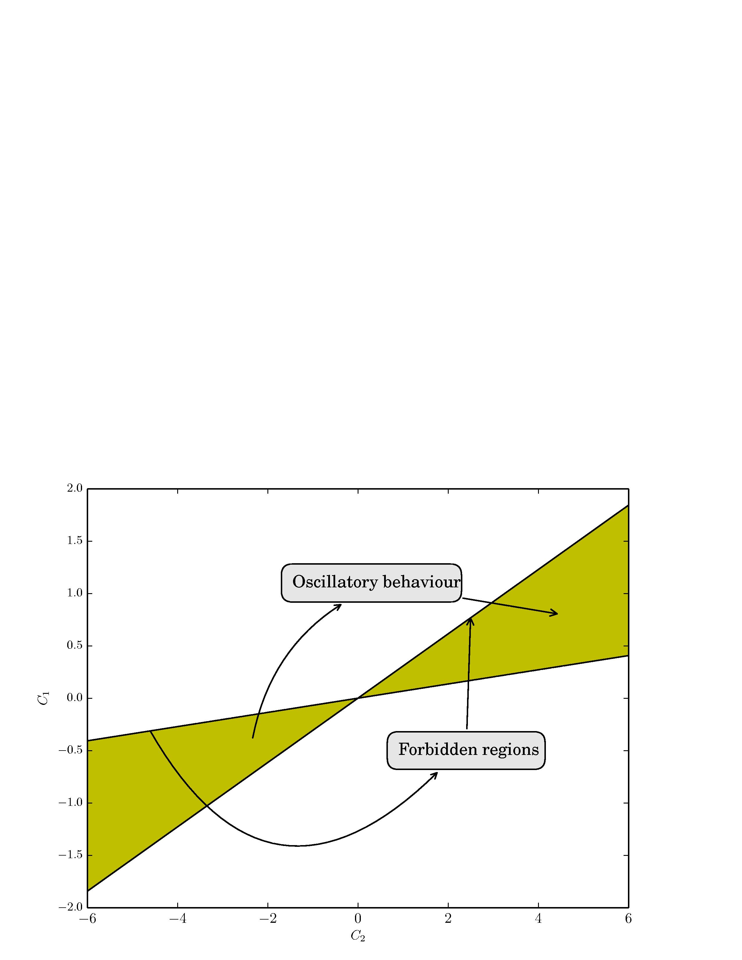
Figure 1: Regions where the behavior of the moduli fields are oscillatory or hyperbolic. The region outside of the oscillatory and forbidden regions correspond to the hyperbolic behavior.

On the other hand, we see that the solution associated to the equation (41b) is the same for all Bianchi Class A cosmological models. It was the main result obtained in Sesma et al. (2016); Socorro and Toledo Sesma (2016). This can be appreciated by observing the Hamiltonian operator (30), which can be split as $\rm\hat{H}(a,c,\phi,\sigma)\Psi=\hat{H}_{g}(a,c)\Psi+\hat{H}_{m}(\phi,\sigma)\Psi=0$, where $\rm\hat{H}_{g}$ y $\rm\hat{H}_{m}$ represents the Hamiltonian for gravitational sector and the moduli fields, respectively, and the scale factors have the transformations $A=e^{a},C=e^{c}$.

With the last results, we obtain the general solution to the WDW equation (40) whose wave function $\Phi$ can be built by taking the superposition of the functions (44) and (45), that is

$$\Psi(A,C,\phi,\sigma)=\mathcal{K}\left(\frac{A}{C^{\beta/\alpha}}\right)^{\alpha}e^{-\frac{2}{\hbar^{2}\alpha}C^{4}}\left(\sin\left[\Lambda(\phi+\sigma)\right]+\cos\left[\Lambda(\phi+\sigma)\right]\right),$$ (46)

where we have taken the constants $G_{0}=1$ and $\{C_{i}\}_{i=1}^{4}=1$ for simplicity, and $\mathcal{K}$ is a constant the allows us to normalize the wave function. The normalization constant $\mathcal{K}$ can be obtained by demanding the condition

$$\int\Psi(A,C,\phi,\sigma)\Psi^{*}(A,C,\phi,\sigma)=1.$$ (47)

V Bohm’s formalism

So far, we have solved the WDW equation (40), and we have found that the wave function $\Psi$ can be split as the product of two wave functions $\Theta$ and $\Phi$, which are given by (44,45). On the other hand, we know that WKB approximation is very important in quantum mechanics and therefore, we shall introduce an ansatz for the wave function $\Psi$ to take the form

$$\Theta(\ell^{\mu})=W(\ell^{\mu})e^{-\frac{S(\ell^{\mu})}{\hbar}},$$ (48)

where $W(\ell^{\mu})$ is an amplitude which varies slowly and $S(\ell^{\mu})$ is the phase whose variation is faster that the amplitude, this allows us to obtain eikonal-like equations. The term $\ell^{\mu}$ is the dynamical variables of the minisuperspace which are $\ell^{\mu}=a,c$. This formalism is known as the Bohm’s formalism too Licata and Fiscaletti (2014); Moniz (2010); Socorro et al. (2012); Bohm (1952).

So, the equation (41a) is transformed under the expression (48) into

$$\hbar^{2}\left[\frac{\partial^{2}W}{\partial a^{2}}-(p+1)\frac{\partial W}{\partial a}-2\frac{\partial^{2}W}{\partial a\partial c}\right]+\hbar\left[-2\frac{\partial W}{\partial a}\frac{\partial S}{\partial a}-W\frac{\partial^{2}S}{\partial a^{2}}+(p+1)W\frac{\partial S}{\partial a}+2\frac{\partial W}{\partial a}\frac{\partial S}{\partial c}+2\frac{\partial W}{\partial c}\frac{\partial S}{\partial a}+2W\frac{\partial^{2}S}{\partial a\partial c}\right]$$

$$+W\left[\left(\frac{\partial S}{\partial a}\right)^{2}-2\left(\frac{\partial S}{\partial a}\right)\left(\frac{\partial S}{\partial c}\right)-(16e^{4c}+C_{1}+\mu^{2})\right]=0,$$ (49)

The last expression (49) can be written as the following set of partial differential equations, as a WKB-like procedure

$$\left(\frac{\partial S}{\partial a}\right)^{2}-2\left(\frac{\partial S}{\partial a}\right)\left(\frac{\partial S}{\partial c}\right)-(16e^{4c}+C_{1}+\mu^{2}) = 0,$$ (50a)

$$-2\frac{\partial W}{\partial a}\frac{\partial S}{\partial a}-W\frac{\partial^{2}S}{\partial a^{2}}+(p+1)W\frac{\partial S}{\partial a}+2\frac{\partial W}{\partial a}\frac{\partial S}{\partial c}+2\frac{\partial W}{\partial c}\frac{\partial S}{\partial a}+2W\frac{\partial^{2}S}{\partial a\partial c} = 0,$$ (50b)

$$\frac{\partial^{2}W}{\partial a^{2}}-(p+1)\frac{\partial W}{\partial a}-2\frac{\partial^{2}W}{\partial a\partial c} = 0.$$ (50c)

This set of equation are solved in a different way with the previous works, because the constraint equation was the equation (50c) in the past, however now is solved in first instance. In this set of equations, the first partial differential equation is known as the Hamilton-Jacobi equation for the gravitational field, with the equation (50c) we obtain the W function, and the the expression (50b) is the constraint equation. From the last system of partial differential equation (50) , we observe that the equation (50c) has a solution given by

$$\rm W(a,c)=\frac{1}{S_{0}^{2}}\left[4S_{4}e^{4c}+(2S_{4}a-S_{5})S_{0}^{2}+S_{4}(C_{1}+\mu^{2}+S_{0}^{2})c\right]e^{-\frac{1+p}{2}c}$$ (51)

and the solutions for the function S are

$$\rm S=S_{0}a+S_{2}c+S_{3}e^{4c},\qquad S_{3}=-\frac{2}{S_{0}},\quad S_{2}=\frac{S_{0}^{2}-C_{1}-\mu^{2}}{2S_{0}},$$ (52)

where $\rm S_{0},S_{4}$ and $\rm S_{5}$ are integration constants. When we introduce these results into the equation (41a), with $\rm\Theta(\ell^{\mu})=W(\ell^{\mu})e^{-\frac{S(\ell^{\mu})}{\hbar}}$, this partial differential equation is satisfy identically.

VI Final Remarks

In this work we have developed the anisotropic Bianchi $VI_{h=-1}$ model from a higher-dimensional theory of gravity, our analysis cover the classical and quantum aspects. In the frame of classical analysis we obtained that two radii of the Bianchi $VI_{h=-1}$ type are proportional, we choose the equality ($\rm B(t)=C(t)$) presenting a hidden symmetry, which say that the volume function of this cosmological model goes as a jet in x direction, whereas in the (y,z) plane goes as a circle. This hidden symmetry allows us to simplify the analysis in the classical context, and as a consequence the quantum version was simplified too. The last result we can compared it with the jet emission that occurs in some stars, in this sense we explore in this context the flat FRW cosmological model, finding that the scale factor goes to the B radii corresponding to Bianchi type VI cosmological model, we can infer that the flat FRW cosmological model is embedded in this anisotropic cosmological Bianchi type model. Concerning to the quantum scheme, we can observe that this anisotropic model is completely integrable with no need to use numerical methods. Some results have been obtained by considering just the gravitational variables in Socorro et al. (2010). On the other hand, we obtain that the solutions in the moduli fields are the same for all Bianchi Class A cosmological models (45), the last conclusion is possible because the Hamiltonian operator in (29) can be written in separated way as $\hat{H}(A,C,\phi,\sigma)\Psi=\hat{H}_{g}(A,C)\Psi+\hat{H}_{m}(\phi,\sigma)\Psi=0$, where $\hat{H}_{g}$ y $\hat{H}_{m}$ are the Hamiltonian for the gravitational sector and the moduli fields, respectively. The full wave function given by $\Psi=\Phi(\phi,\sigma)\Theta(A,C)$ is a superposition of the gravitational variables and the moduli fields. There are some recent research related on this line Alves-Júnior et al. (2016), they built a wave packet for an arbitrary anisotropic background. However, one of the main problem in quantum cosmology is how to built a wave packet that allows to determine the possible states of the classical universe Bojowald (2011); Halliwell (1990); DeWitt (1967); Lemos (1996); Blyth and Isham (1975); Farajollahi et al. (2010); Letelier and Pitelli (2010); Vakili (2012); Chodos and Detweiler (1980).

Appendix A The Explicit Einstein’s equations

The Einstein’s equations and the equation of motions are given by the expressions (6). In detail they are

$$G^{0}_{0}: \frac{\dot{A}}{NA}\frac{\dot{B}}{NB}+\frac{\dot{A}}{NA}\frac{\dot{C}}{NC}+\frac{\dot{B}}{NB}\frac{\dot{C}}{NC}-\left(\frac{\dot{\phi}}{N}\right)^{2}-18\frac{\dot{\phi}}{N}\frac{\dot{\sigma}}{N}-48\left(\frac{\dot{\sigma}}{N}\right)^{2}-8\pi G\rho-\frac{1}{A^{2}}=0,$$ (53a)

$$G^{0}_{1} = -G^{1}_{0}:\frac{\dot{B}}{NB}-\frac{\dot{C}}{NC}=0,$$ (53b)

$$G^{1}_{1}: \frac{\ddot{B}}{N^{2}B}+\frac{\ddot{C}}{N^{2}C}+\frac{\dot{B}}{NB}\frac{\dot{C}}{NC}-\frac{\dot{B}}{NB}\frac{\dot{N}}{N^{2}}-\frac{\dot{C}}{NC}\frac{\dot{N}}{N^{2}}+\left(\frac{\dot{\phi}}{N}\right)^{2}+18\frac{\dot{\phi}}{N}\frac{\dot{\sigma}}{N}+48\left(\frac{\dot{\sigma}}{N}\right)^{2}$$ (53c)

$$+8\pi Gp+\frac{1}{A^{2}}=0,$$

$$G^{2}_{2}: \frac{\ddot{A}}{N^{2}A}+\frac{\ddot{C}}{N^{2}C}+\frac{\dot{A}}{NA}\frac{\dot{C}}{NC}-\frac{\dot{A}}{NA}\frac{\dot{N}}{N^{2}}-\frac{\dot{C}}{NC}\frac{\dot{N}}{N^{2}}+\left(\frac{\dot{\phi}}{N}\right)^{2}+18\frac{\dot{\phi}}{N}\frac{\dot{\sigma}}{N}+48\left(\frac{\dot{\sigma}}{N}\right)^{2}$$ (53d)

$$+8\pi Gp-\frac{1}{A^{2}}=0,$$

$$G^{3}_{3}: \frac{\ddot{A}}{N^{2}A}+\frac{\ddot{B}}{N^{2}B}+\frac{\dot{A}}{NA}\frac{\dot{B}}{NB}-\frac{\dot{A}}{NA}\frac{\dot{N}}{N^{2}}-\frac{\dot{B}}{NB}\frac{\dot{N}}{N^{2}}+\left(\frac{\dot{\phi}}{N}\right)^{2}+18\frac{\dot{\phi}}{N}\frac{\dot{\sigma}}{N}+48\left(\frac{\dot{\sigma}}{N}\right)^{2}$$ (53e)

$$+8\pi Gp-\frac{1}{A^{2}}=0,$$

$$\Box\phi=0: \left(\frac{\dot{A}}{NA}+\frac{\dot{B}}{NB}+\frac{\dot{A}}{NA}+\frac{\dot{C}}{NC}\right)\frac{\dot{\phi}}{N}+\frac{\ddot{\phi}}{N^{2}}-\frac{\dot{\phi}}{N}\frac{\dot{N}}{N^{2}}=0,$$ (53f)

$$\Box\sigma=0: \left(\frac{\dot{A}}{NA}+\frac{\dot{B}}{NB}+\frac{\dot{A}}{NA}+\frac{\dot{C}}{NC}\right)\frac{\dot{\sigma}}{N}+\frac{\ddot{\sigma}}{N^{2}}-\frac{\dot{\sigma}}{N}\frac{\dot{N}}{N^{2}}=0.$$ (53g)

The expressions that involve $\dot{q}$ means derivative with respect to the cosmic time, and the relation between the cosmic and proper times is given by

$$d\tau=N(t)\,dt,$$ (54)

With the last consideration we see that is possible to rewrite the last system of differential equations (53) as follows

$$\dot{\phi}=N\phi^{\prime},\qquad\ddot{\phi}=N^{2}\phi^{\prime\prime}+\dot{N}\phi^{\prime},$$ (55)

just to to mention the transformation of the scalar field. Under this change, we see that the system (53) can be transformed into

$$G^{0}_{0}: 2\frac{A^{\prime}C^{\prime}}{AC}+\biggl{(}\frac{C^{\prime}}{C}\biggr{)}^{2}-\phi^{\prime 2}-18\phi^{\prime}\sigma^{\prime}-48\sigma^{\prime 2}-8\pi G\rho-\frac{1}{A^{2}}=0,$$ (56a)

$$G^{1}_{1}: 2\frac{C^{\prime\prime}}{C}+C^{\prime 2}+\phi^{\prime 2}+18\phi^{\prime}\sigma^{\prime}+48\sigma^{\prime 2}+8\pi Gp+\frac{1}{A^{2}}=0,$$ (56b)

$$G^{2}_{2}=G^{3}_{3}: \frac{A^{\prime\prime}}{A}+\frac{C^{\prime\prime}}{C}+A^{\prime}C^{\prime}+\phi^{\prime 2}+18\phi^{\prime}\sigma^{\prime}+48\sigma^{\prime 2}+8\pi Gp-\frac{1}{A^{2}}=0,$$ (56c)

$$\Box\phi=0: 2\,\left(\frac{A^{\prime}}{A}+\frac{C^{\prime}}{C}\right)\phi^{\prime}+\phi^{\prime\prime}=0,$$ (56d)

$$\Box\sigma=0: 2\,\left(\frac{A^{\prime}}{A}+\frac{C^{\prime}}{C}\right)\sigma^{\prime}+\sigma^{\prime\prime}=0,$$ (56e)

where we have use that the scale factors $B(t)$ and $C(t)$ are equal. This result can be obtained from the expression (53b), whose differential equation can be transformed into the proper time as

$$\frac{B^{\prime}}{B}-\frac{C^{\prime}}{C}=0\implies\frac{d}{dt}\ln B-\frac{d}{dt}\ln C=0\implies\frac{d}{dt}\ln\left(\frac{B}{C}\right)=0\implies\ln\left(\frac{B}{C}\right)=1.$$ (57)

In the last expression we have fixed that the integration constant equal to one.

References

Ade et al. (2016)
P. A. R. Ade
et al. (Planck),
Astron. Astrophys. 594,
A18 (2016), eprint 1502.01593.
Socorro and Toledo Sesma (2016)
J. Socorro and
L. Toledo Sesma,
Eur. Phys. J. Plus 131,
71 (2016), eprint 1507.03171.
Sesma et al. (2016)
L. T. Sesma,
J. Socorro, and
O. Loaiza,
Adv. High Energy Phys. 2016,
6705021 (2016), eprint 1501.02779.
Kiefer (2000)
C. Kiefer, in
Towards quantum gravity
(Springer, 2000), pp.
158–187.
Isham (1993)
C. J. Isham, in
Integrable systems, quantum groups, and quantum
field theories (Springer, 1993), pp.
157–287.
Alvarenga et al. (2002)
F. G. Alvarenga,
J. C. Fabris,
N. A. Lemos, and
G. A. Monerat,
Gen. Rel. Grav. 34,
651 (2002), eprint gr-qc/0106051.
Alves-Júnior
et al. (2016)
F. A. P. Alves-Júnior,
M. L. Pucheu,
A. B. Barreto,
and C. Romero
(2016), eprint 1611.03812.
Obregón and Socorro (1996)
O. Obregón and
J. Socorro,
Int. J. of Theor. Phys. 35,
1381 (1996), eprint 9506021.
Socorro (2003)
J. Socorro,
Int. J. Theor. Phys. 42,
2087 (2003), eprint gr-qc/0304001.
Chowdhury and Mathur (2007)
B. D. Chowdhury
and S. D.
Mathur, Class. Quant. Grav.
24, 2689 (2007),
eprint hep-th/0611330.
Kiefer (2007)
C. Kiefer,
Quantum Gravity (Oxford
University Press, New York, 2007), ISBN
9780199212521.
Moniz (2010)
P. V. Moniz,
Quantum Cosmology-The Supersymmetric Perspective-Vol.
1: Fundamentals, vol. 803 (Springer,
2010).
Gibbons and Grishchuk (1989)
G. W. Gibbons and
L. P. Grishchuk,
Nucl. Phys. B313,
736 (1989).
Hartle and Hawking (1983)
J. B. Hartle and
S. W. Hawking,
Phys. Rev. D28,
2960 (1983).
Fang and Ruffini (1987)
L. Fang and
R. Ruffini,
Quantum Cosmology, Advanced series in astrophysics
and cosmology (World Scientific, 1987).
Licata and Fiscaletti (2014)
I. Licata and
D. Fiscaletti,
Quantum potential: Physics, geometry and algebra
(Springer, 2014).
Socorro et al. (2012)
J. Socorro,
P. A. Rodríguez,
O. Núñez-Soltero,
R. Hernández,
and
A. Espinoza-García,
Quintom Potential from Quantum Anisotropic Cosmological
Models (Open Questions in Cosmology,
2012).
Bohm (1952)
D. Bohm, Phys.
Rev. 85, 166
(1952).
Socorro et al. (2010)
J. Socorro,
M. Sabido,
M. A. Sanchez G.,
and M. G. F.
Palos, Rev. Mex. Fis.
56, 166 (2010),
eprint 1007.3306.
Bojowald (2011)
M. Bojowald,
Quantum cosmology: a fundamental description of the
universe, vol. 835 (Springer Science
& Business Media, 2011).
Halliwell (1990)
J. J. Halliwell,
” Introductory lectures on quantum cosmology., by
Halliwell, JJ. Massachusetts Inst. of Tech., Cambridge (USA). Center for
Theoretical Physics, Mar 1990, 54 p., To appear in” Proceedings of the
Jerusalem Winter School on Quantum Cosmology and Baby Universes” edited by T.
Piran, 1990.” 1 (1990).
DeWitt (1967)
B. S. DeWitt,
Phys. Rev. 160,
1113 (1967).
Lemos (1996)
N. A. Lemos,
Phys. Rev. D53,
4275 (1996), eprint gr-qc/9509038.
Blyth and Isham (1975)
W. F. Blyth and
C. J. Isham,
Phys. Rev. D11,
768 (1975).
Farajollahi et al. (2010)
H. Farajollahi,
M. Farhoudi, and
H. Shojaie,
Int. J. Theor. Phys. 49,
2558 (2010), eprint 1008.0910.
Letelier and Pitelli (2010)
P. S. Letelier and
J. P. M. Pitelli,
Phys. Rev. D82,
104046 (2010), eprint 1010.3054.
Vakili (2012)
B. Vakili,
Phys. Lett. B718,
34 (2012), eprint 1208.4083.
Chodos and Detweiler (1980)
A. Chodos and
S. L. Detweiler,
Phys. Rev. D21,
2167 (1980).