Deep Residual Learning for Accelerated MRI using Magnitude and Phase Networks
Abstract
Objective: Accelerated magnetic resonance (MR) scan acquisition with compressed sensing (CS) and parallel imaging is a powerful method to reduce MR imaging scan time. However, many reconstruction algorithms have high computational costs. To address this, we investigate deep residual learning networks to remove aliasing artifacts from artifact corrupted images. Methods: The deep residual learning networks are composed of magnitude and phase networks that are separately trained. If both phase and magnitude information are available, the proposed algorithm can work as an iterative k-space interpolation algorithm using framelet representation. When only magnitude data is available, the proposed approach works as an image domain post-processing algorithm. Results: Even with strong coherent aliasing artifacts, the proposed network successfully learned and removed the aliasing artifacts, whereas current parallel and CS reconstruction methods were unable to remove these artifacts. Conclusion: Comparisons using single and multiple coil show that the proposed residual network provides good reconstruction results with orders of magnitude faster computational time than existing compressed sensing methods. Significance: The proposed deep learning framework may have a great potential for accelerated MR reconstruction by generating accurate results immediately.
Index Terms:
Compressed sensing MRI, Deep convolutional framelets, Deep learning, Parallel imagingI Introduction
Magnetic resonance imaging (MRI) is one of the most valuable imaging methods for diagnostic and therapeutic indications. However, physical and physiological constraints limit the rate of magnetic resonance (MR) scan acquisition. One of the main MRI shortcomings is the long scan, hence accelerated MR acquisition is important to reduce scan time. Hence, k-space under-sampling is often required, and various reconstruction methods have been developed, including parallel MRI (pMRI) [1, 2] and compressed sensing (CS) MRI (CS-MRI) [3, 4] to provide accurate reconstruction from insufficient k-space samples.
Generalized auto-calibrating partial parallel acquisition (GRAPPA) [2] is a representative pMRI technique that interpolates the missing k-space data by exploiting the diversity of coil sensitivity maps. CS-MRI reconstructs a high resolution image from randomly subsampled k-space data, utilizing data sparsity in the transformed domain. These algorithms are usually combined to provide acceleration [5, 6].
Recent algorithms convert CS-MRI and/or pMRI problem to a k-space interpolation problem using a low rank structured matrix completion, e.g. SAKE [7] and the annihilating filter-based low rank Hankel matrix approach (ALOHA) [8, 9, 10, 11], producing state-of-the-art reconstruction performance. However, the algorithms are limited by their computational complexity, and CS algorithms require access to the k-space data, so the quality improvement in the image domain using post processing techniques is not possible.
Deep learning is an important framework for computer vision research [12] thanks to the availability of massive datasets and high performance computing hardware, such as graphic processor unit (GPU). In particular, convolutional neural networks (CNNs) train convolution filters to effectively extract features from the training data, with great successes in classification [12], and regression problems, such as segmentation [13], denoising [14, 15], super resolution [16, 17, 18], etc. Therefore, the current study utilized deep CNN to capture image structure features for medical image reconstruction.
Wang et al [19] applied deep learning to CS-MRI, training the CNN from down-sampled reconstruction images to learn fully sampled reconstruction. They then used the deep learning result as either an initialization or regularization term in classical CS approaches. A multilayer perceptron was proposed for accelerated pMRI [20], and deep CNN architecture using an unfolded iterative CS algorithm was proposed in [21], where trained optimal regularizers were proposed in contrast to the usual approach using handcrafted regularizers [21]. Kang et al [22] provided the first systematic study of deep CNN for low dose x-ray computed tomography (CT), and showed that a deep CNN using directional wavelets was more efficient in removing low dose related CT noise.
However, in contrast to low dose artifacts from reduced tube currents, streaking originating from sparse projection views are globalized artifacts and difficult to remove using conventional denoising CNNs. Han et al [23] and Jin et al [24] independently proposed multi-scale residual learning networks using U-Net [13] to remove these global streaking artifacts, and domain adaptation from CT to MRI has been also successfully demonstrated [25]. These pioneering works show the significant potential of deep learning for image reconstruction.
The residual network (ResNet) [26] has been recently studied in the context of image classification. The gradient can be backpropagated into much deeper layers due to the identity mapping path in the residual network, which enables very deep residual network structure [26]. Therefore, we investigated ResNet based image reconstruction to deal with complex-valued MR data, and propose a new scheme to train phase and magnitude separately. An important advantage of the proposed approach is that the algorithm does not require any k-space data for magnitude-only images, because the processing can be done in the image domain as an image restoration task. If both phase and magnitude information are available, the proposed algorithm works as an iterative k-space interpolation algorithm using framelet representation [27, 28]. Based on recent deep convolutional framelet theory, we employ a multi-scale network structure (called dual frame U-net) [29] to correct globalized artifacts from under-sampled k-space data. Numerical experiments confirmed the effectiveness of the proposed deep learning approach for CS and pMRI.
II Related Studies
Consider a two-dimensional (2D) acquisition scenario where a 2D image , is reconstructed from a Fourier transform (FT) on k-space coordinates . The k-space data from the -th coil can be represented as
| (1) |
where is the coil sensitivity of the -th coil, and is the number of the coils. The operator notation for (1) is
where is a diagonal operator of the -th coil sensitivity.
Only a subset of k-space measurements are obtained for accelerated MRI. For a given subsampling pattern , let be the diagonal matrix with 1 for indices in and 0 otherwise. Then, the standard reconstruction approach is to solve the penalized least squares minimization problem
| (2) |
where denotes regularization terms, such as the total variation penalty, etc. When the sensitivity map is unknown, direct estimation of sensitivity weighted images can be expressed as
| (3) |
For example, - iterative self-consistent parallel imaging reconstruction (-SPIRiT) [30] utilizes additional GRAPPA type constraints for the CS problem
| subject to | ||||
where
| (4) |
denote the unknown images and their k-space measurements for the given set of coils, respectively; denotes the -mixed norm of a matrix; denotes a discrete wavelet transform matrix; and is an image domain GRAPPA operator. This problem can be solved using proximal algorithms.
III Main Contributions
III-A Magnitude and Phase Networks
We are interested in solving accelerated MR reconstruction problems using k-space interpolation. The concept was inspired by classical frame based inpainting approaches [27, 28]. Let be the mapping that satisfy perfect reconstruction (PR), i.e.,
| (5) |
where is the fully sampled k-space samples from multiple coils. Then, we have the identity
| (6) |
where denotes that the measurement in (4) are measured on . To avoid the trivial solution, mapping should include the shrinkage operator. Equation (6) can be expressed as an iterative -space interpolation algorithm
| (7) |
Since MRI uses FT, , (5) can be expressed as
| (8) |
corresponding to PR image domain. Therefore, we want to find the image domain mapping . The reason we prefer in the image domain is that image domain networks have been widely investigated in the context of computer vision, whereas to the best of our knowledge, k-space domain networks has not be previously investigated.
Here, we must consider the complex nature of MR images to impose constraint (8). Hence, we represent mapping (8) as
| (9) |
where and denote magnitude and phase mapping, respectively. This approach has many advantages. Magnitude-only images are used for many clinical applications, and users process data from an image workstation that does not have access to the raw k-space data. Hence, the magnitude network works as a post-processing algorithm to improve the image. Furthermore, many public datasets, such as the Human Connectome Project (HCP) dataset (https://db.humanconnectome.org), are in the form of magnitude images, which can be used to pre-train the magnitude network.
On the other hand, when phase information is available due to the access to the complex images, then combining the phase domain network allows exploiting iterative k-space interpolation using (7), which is summarized in Algorithm 1. Algorithm 1 is a relaxed iteration using the Krasnoselskii-Mann (KM) method [31] to improve frame based interpolation iteration convergence.
Therefore, the remaining issue is how to design the magnitude and phase networks, and , respectively. This is discussed in Section III C.
III-B Network Architecture

(a)

(b)
One of the most widely used deep learning network architecture for inverse problems is U-net [24, 25], which incorporates bypass connection and pooling/unpooling layers. Figure 2(a) shows an example one-dimensional (1D) U-Net. However, U-net has limitations due to duplication of low frequency content [32]. Therefore, we employ the dual frame U-net [29], as shown in Fig. 2(b) to overcomes this limitation. In contrast to U-net, the residual signal at low resolution is up-sampled through the unpooling layer and subtracted to remove duplicated low frequency content. This can be implemented using an additional bypass connection for the low resolution signal, as shown in Fig. 2(b). See Appendix -B and [29] for detailed descriptions regarding why and how to employ dual frame U-Net. In addition to the application of dual frame U-Net for sparse CT reconstruction problems [29], dual frame U-Net has been successfully used for elastic source imaging problems [33], a complicated inverse scattering problem, confirming the advantages of dual frame U-Net over U-Net. Therefore, we propose dual frame U-Net for MR reconstruction.
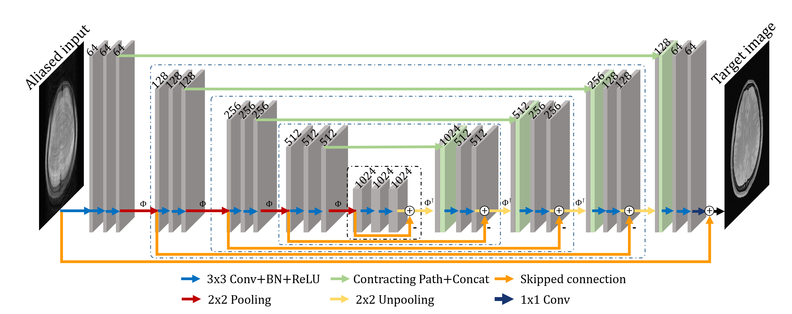
Figure 1 shows the 2D extension of Fig. 2(b). Since there is a skipped connection at the output level, this is referred to as a residual network. The proposed residual network consists of a convolution layer, batch normalization [34], rectified linear unit (ReLU) [12], and contracting path connection with concatenation [13]. Each stage contains four sequential layers comprising convolution with kernels, batch normalization, and ReLU layers. The final layer only contains a convolution with kernel. Figure 1 shows the number of channels for each convolution layer. Using pooling layers, the proposed network has five representation scales, as shown in Fig. 1, where the number of channels after each pooling layer is doubled. Input resolution is , and the representation resolution is halved for each scale change until it becomes in scale 4. The pooling layers mean the receptive field in the multi-scale network increases exponentially. Consequently, the dual frame U-net structure produces a larger receptive field, which is useful to capture global artifact patterns.
III-C Reconstruction Flow
The networks for the reconstruction of magnitude and phase have the same architecture as shown in Fig. 1. To train the network, we first apply the inverse Fourier transform to the down-sampled k-space data to generate aliased images. Inputs for the magnitude network were the magnitude of distorted MR images and targets were the alias-free image magnitudes. Phase reconstruction was similarly trained with distorted and alias-free image phases, respectively.
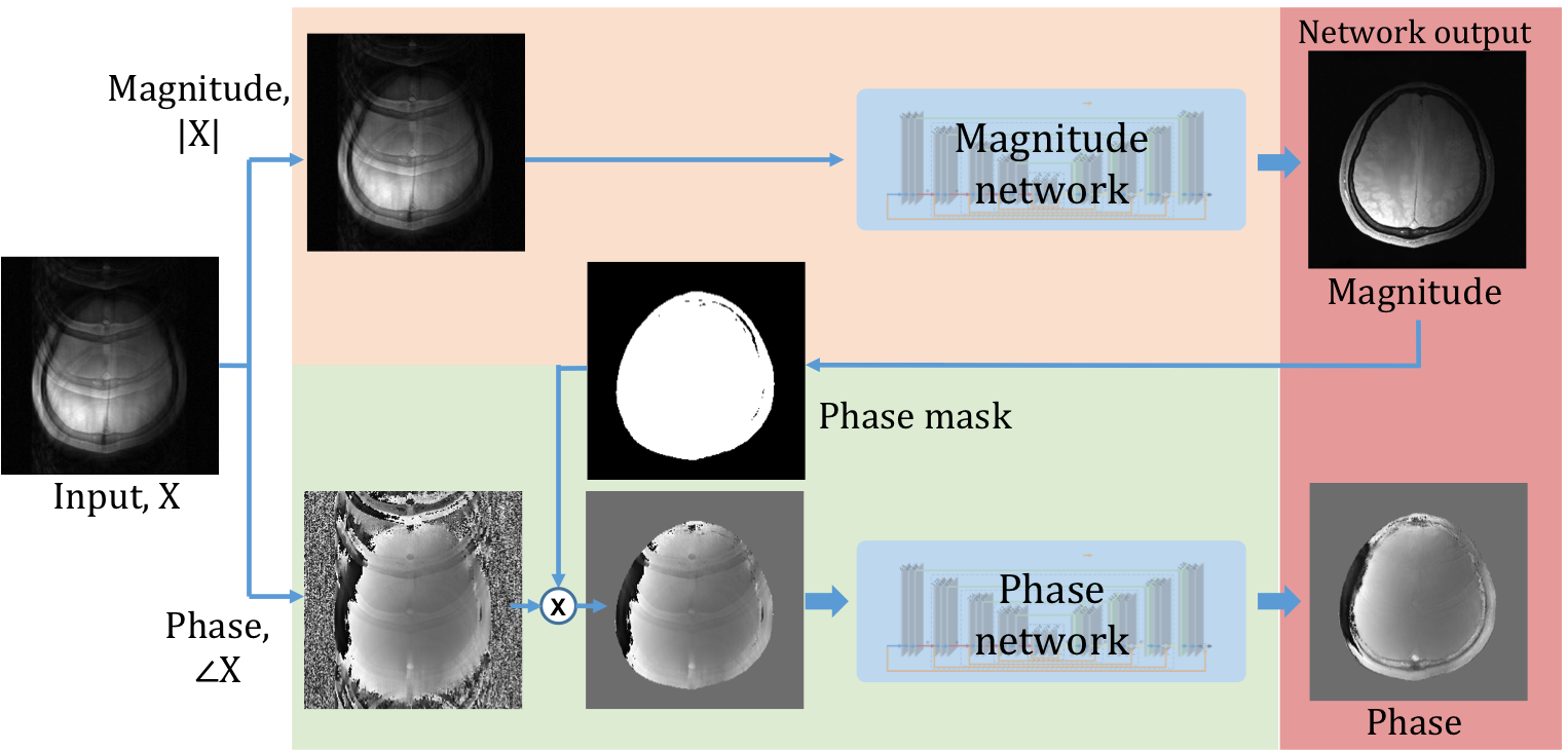
Although both networks have the same structure, there is an additional step for the phase network. The phase image of Figure 3 (bottom row) shows that the phase image region within the brain has smooth structures with slowly varying pixel values from to , whereas the region outside the brain has approximately zero magnitude, but large phase fluctuations, since the pixels have random values from to . These random phases outside the brain region complicate network training. One advantage of separate phase estimation is that the spatial support information from the magnitude network can be used to improve phase reconstruction. Therefore, we use phase masking to eliminate these random phase effects outside the brain.
Thus, we first trained the magnitude network, and then obtained phase masks from reconstructed magnitude images using a simple threshold. We set phase outside the ROI (as defined by the phase masks) to zero for both input and artifact phase images, eliminating random phase effects outside the brain. The phase network is then trained using artifact-free phase data within the phase mask as targets.
After training the networks, the inference of the networks follows the same steps as the training process (Fig. 3). Since the phase masks should be generated before phase reconstruction, we first reconstruct magnitude images using the trained magnitude network (Fig. 3, orange box). The phase mask indicating the brain area is then generated by thresholding the reconstructed magnitude image, and phase outside the phase mask is removed before being applied to the phase network (Fig. 3, green box). For the multi-channel case, the square root of sum of squares (SSOS) image was calculated after reconstruction.
If phase information is available, we can use Algorithm 1 to improve reconstruction. Due to the recursive nature of the network, the following iterative training procedure was used. The magnitude and phase network are trained on the initial training database, and missing k-space measurements are estimated. We then augment measured k-space data with estimated k-space data, and obtain reconstructed images by FT. These images are used as an additional dataset for further magnitude and phase network training. Thus, the networks learn the mapping not only from strongly aliased input, but also from almost artifact-free images. For the inference of the networks, in Algorithm 1 is set to decrease from 1 to 0, and is set to 1.
The theoretical background for the proposed training using both strongly aliased and near artifact-free images is from the framelet nature of deep CNNs, which was the main outcome from the mathematical theory in our companion paper [32] (see Appendix A for the review). Neural network training learns framelet bases from the training data that best represent the signals. Thus, the learned bases should be sufficiently robust to provide good representation for the given input data set. In the KM iteration, each iterative step provides improved images, which should be input to the same neural network. Thus, framelet bases should be trained to be optimal not only for strongly aliased input but also for near artifact-free images. Similar training techniques are implicitly used for recursive neural networks (RNN) after unfolding [35].
IV Method
IV-A Magnetic Resonance Dataset
We used three brain image datasets, including structural MRI images from the HCP dataset, to increase the magnitude network training dataset; and two in vivo k-space datasets from 3T and 7T scanners. We select 200 of the 1200 HCP T2 weighted structural images to pre-train the magnitude network. The data set were collected using the 3D T2-SPACE sequence with TR 3200 ms, TE 565 ms, variable flip angle, FOV 224224 mm, and 32 channel head coils. A total of 12,000 slices of the HCP dataset were used for pre-training. Since the HCP T2 weighted image was obtained as the SSOS from the multi-coil reconstruction, we generated simulated coil magnitude images by multiplying the sensitivity maps extracted from 3T and 7T in vivo MR datasets.
Although public dataset such as HCP can be used to pre-train the magnitude network, phase variations in MR images are usually small, and a small number of in vivo data are usually sufficient to train the phase network. Therefore, the phase network was not pre-trained.
The in vivo data 3T MR dataset comprised 81 axial brain slices from nine subjects. Images from seven subjects were used for training (61 images), one subject for validation (8 images), and the final subject (12 images) for testing. Data were acquired in Cartesian coordinates from a 3T MR scanner with four Rx coils (Siemens, Verio). Spin echo (SE) and gradient echo (GRE) scans used TR 3000–4000 ms, TE 4 20 ms, FA , slice thickness 5 mm, 256256 acquisition matrix, four coils, FOV 240240 mm, and anterior to posterior PE direction. Brain images in the dataset had different intensity and maximum scales, since they were acquired with various scan conditions (GRE/SE, various TE/TR, etc.). We selected the first coil data (of four) for single-channel experiments, and used all the coil images for parallel imaging experiments.
IV-B Down-Sampled Data Generation
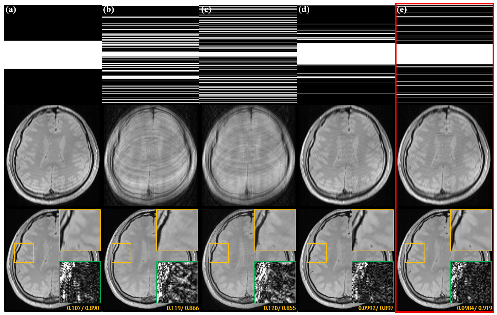
The original k-spaces were retrospectively down-sampled, according to several under-sampling patterns. We compared five sampling patterns to identify any performance effects that differed regarding the ACS lines and distribution type (Gaussian and random), as shown in Fig. 4 (top row). Additional low frequency auto-calibration signal (ACS) lines were required to ensure that aliasing artifacts were primary high frequency signals rather than low frequency repetitions. ACS lines were also necessary for GRAPPA reconstruction for comparative studies. The acceleration factor was set to 3.5 for all sampling patterns.
Normalization is an important preprocessing step to improve reconstruction performance. Since the images were acquired under various scan conditions, the data was normalized separately for each image. Input data for the magnitude network were normalized using scaling factor , where is the maximum image pixel intensity, ensuring input image magnitude was limited to [0,256]. Phase images were already normalized from to , but we modified the range to [0,2] for better reconstruction performance.
Data augmentation was essential for the in vivo data set to make the network more robust. Hence, the original full-sampled images were transformed by flipping to produce augmented MR images. The transforms were performed on the complex image domain to retain full and down-sampled k-space data for the augmented MR images. Thus, 4 more training samples were generated from in vivo k-space data for augmentation.
IV-C Network Training
The network was implemented in MATLAB 2015a using the MatConvNet toolbox (version 23) [36] (Mathworks, Natick). We used a GTX 1080 graphic processor and i7-4770 CPU (3.40 GHz). The convolutional layer weights were initialized by Gaussian random distribution using Xavier s method [37] to obtain an appropriate proper scale. This avoided the signal exploding or vanishing in the initial training phase. We chose the loss function and stochastic gradient descent (SGD) method with momentum to train the weights by minimizing the loss function. Early stopping was used as regularization to avoid overfitting.
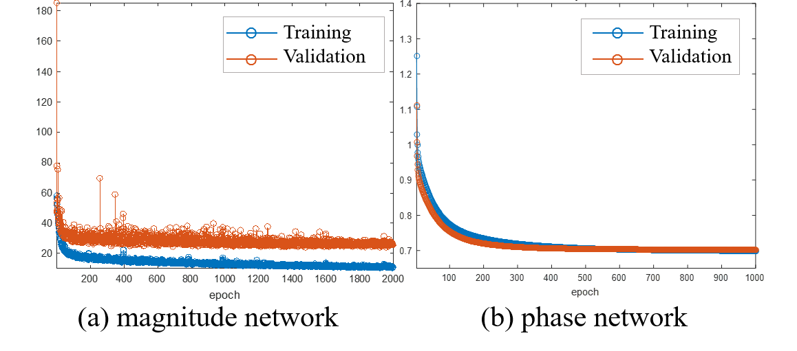
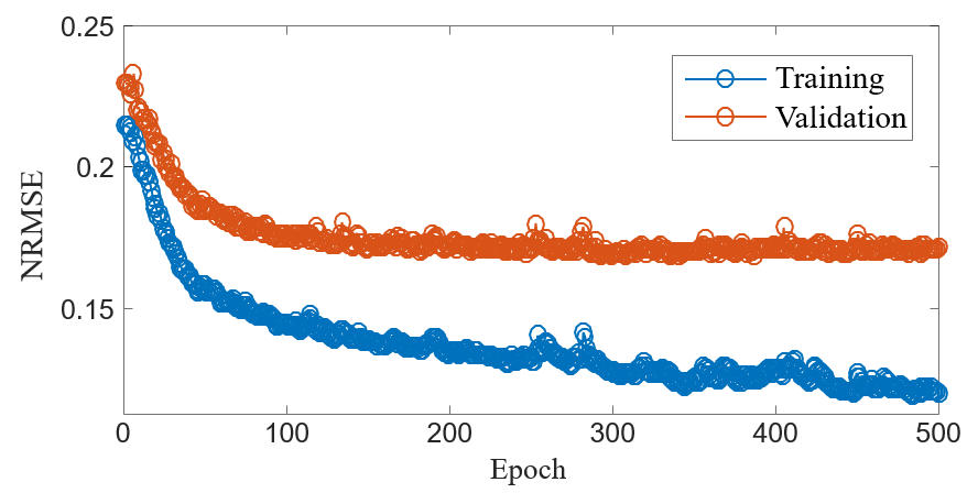
To use the public HCP data set, the training step was divided into three steps: the first 90 epochs for pre-training using the HCP data set, the next 1410 epochs for 3T or 7T in vivo data, and the final 500 epochs for recursive training. Learning rate was reduced logarithmically from to each epoch. The number of epochs for phase network training was set to 1000 due to the relatively simpler structures of phase compared to magnitude, and mini-batch size was set to 10. Figure 5 shows the phase and magnitude network training convergence curves. Training each network for the 3T and 7T MR datasets took approximately 14 and 20 hours, respectively, including pre-training and iterative training using the reconstructed images for KM iteration. Pre-training took approximately 7–8 hours for the HCP dataset.
IV-D Comparative Studies
We used the ALOHA [8] reconstruction as a representative CS algorithm for both single and multi-channel reconstruction to verify network performance. We also compared the reconstruction results for multi-channel dataset with those of GRAPPA [2]. Since GRAPPA is designed for uniform sampling, the GRAPPA reconstruction was performed for uniform sampled k-space with the same ACS lines and same acceleration factor (). The kernel was chosen for the GRAPPA reconstruction, and the following parameters were used for the ALOHA: filter size , , two-stage pyramidal decomposition, tolerance set [0.1, 0.01], and spline wavelet for k-space weighting.
We used SSOS on output magnitude images for final reconstruction as the objective comparison, and SSOS of alias-free reconstruction as the ground-truth,
where refers to the estimated -th coil image, and denotes the number of coils. Phase images reconstructed from the full k-space data were used as phase space ground-truth.
Reconstruction performance was measured by the normalized root mean square error,
where and refer to the estimate and ground-truth images, respectively; denotes the number of pixels; and is the mean value of ; and the structural similarity index [38]
where ; and
and
are the luminance, contrast, and structural terms, respectively, where are the local mean, standard deviation, and cross-covariance for images and , and and are predefined constants [38].
V Experimental Results
We first investigated reconstruction performance depending on various sampling patterns. Figure 4 shows the corresponding aliased input and final reconstruction results (center and bottom rows, respectively). The 20% ACS lines were better than reconstruction results using 5% ACS lines and low frequency sampling, with uniform slightly better than Gaussian random sampling. Therefore, we employed uniform random sampling with 20% ACS lines for all subsequent experiments.
(a)

(b)
We compared a baseline approach to handle the complex data and verify that separate magnitude and phase network training did not degrade performance. The baseline approach stacked the real and imaginary values as two-channel inputs to the neural network and learned the two-channel output consisting of real and imaginary images. After the reconstruction of real and imaginary images, complex valued images were obtained by combining real and imaginary valued images. The inputs were normalized in the same manner, with real and imaginary values [-256,256]. The real and image parts be negative, in contrast to the magnitude network that has only non-negative values. The baseline network architecture was exactly the same as the proposed network (Fig. 1), except that the input and labels were two-channels of real and image components of down-sampled and fully sampled reconstruction, respectively. The network was trained using exactly the same training dataset and procedure, and Fig. 6 shows the convergence.
Magnitude Phase NRMSE SSIM NRMSE SSIM Input 0.237 0.867 0.136 0.986 Complex-net 0.154 0.903 0.111 0.989 Proposed 0.155 0.914 0.111 0.990
Table I shows that the baseline and proposed networks have similar performance, although the proposed network has slight better SSIM. Therefore, considering the advantages of separate magnitude and phase image training, we used the proposed magnitude and phase network structures for subsequent study.
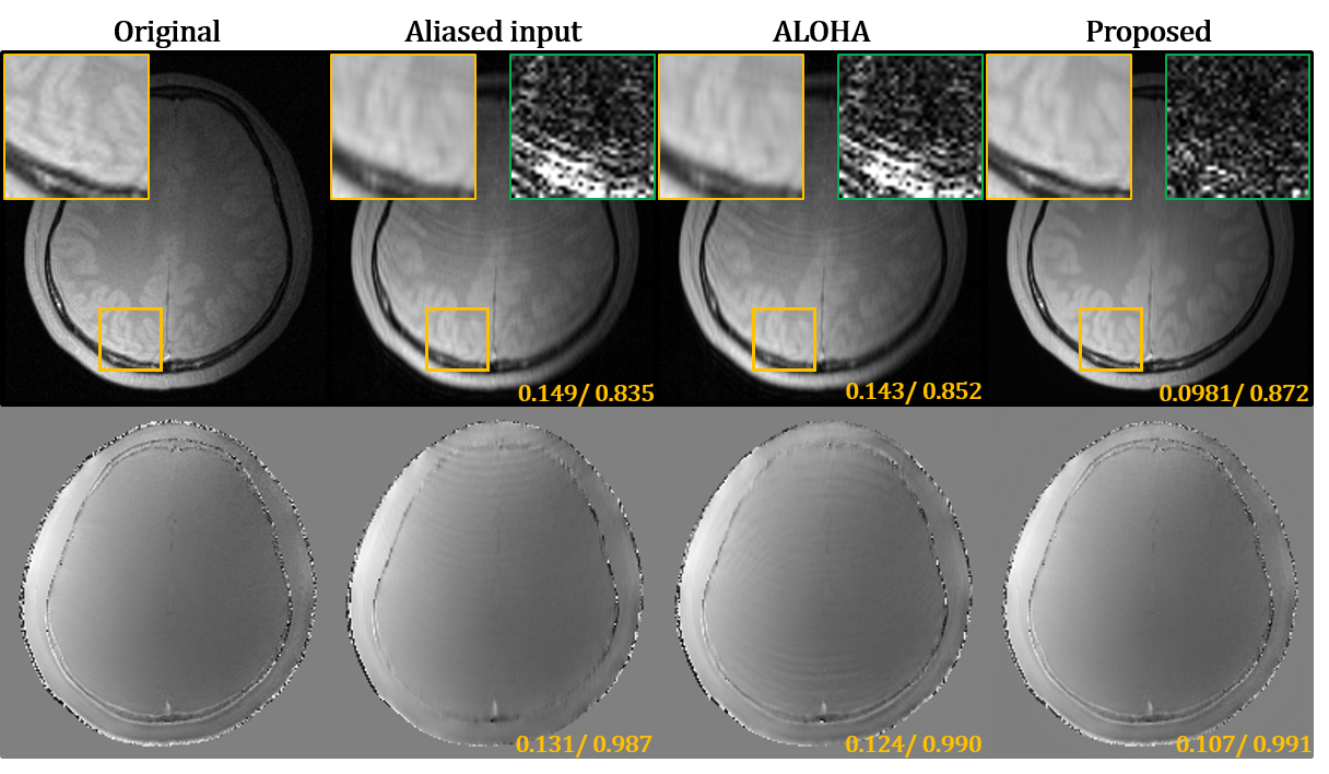
Performance of the proposed network performance was compared with that of ALOHA and GRAPPA to demonstrate the competitive edge against CS and parallel imaging approaches, as shown in Fig. 7. Fig. 7(a) shows that single channel images had significant aliasing artifacts in the input image. However, the aliasing artefacts were mainly for edge images due to the additional ACS lines. The ALOHA approach was somewhat successful with some remaining aliasing artifacts, and the ALOHA reconstruction image was better than the input. However, the result still has aliasing artifacts. In contrast, the approach produced accurate reconstruction, removing aliasing artifacts and has minimum NRMSE.
Fig. 7(b) shows parallel imaging experiments with four channel data. GRAPPA reconstruction exhibits many reconstruction errors, and although ALOHA reconstruction removed many aliasing artifacts, the results were not perfect. In contrast, the proposed method provided excellent reconstruction.
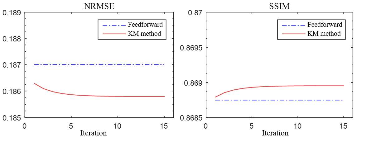
Table II summarizes performance metrics for pre-training using HCP data and iterative update using KM iteration. Pre-training using large datasets improves network reconstruction performance. KM iteration provided minimum NRMSE and maximum SSIM, as shown in Fig. 8.
No. Training method NRMSE SSIM (A) No HCP data pre-training 0.191 0.861 (B) HCP data pre-training 0.187 0.869
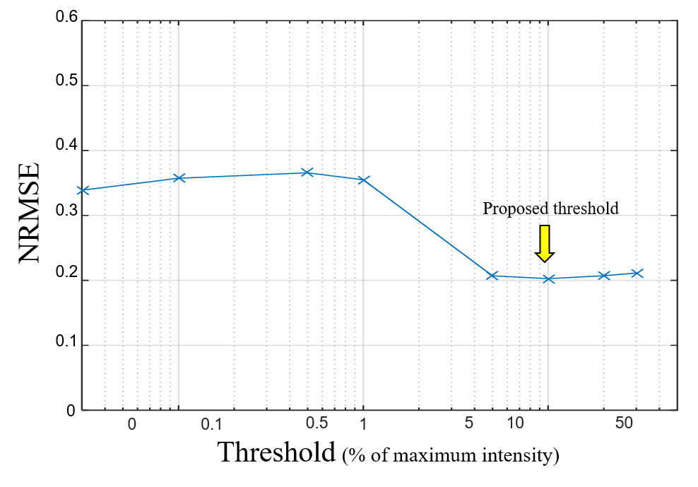
Since the proposed phase network requires a phase mask by thresholding the magnitude network, phase reconstruction accuracy may be sensitive to the chosen threshold. Therefore, the phase network was trained under various phase masking levels: 0, 0.1, 0.5, 1, 5, 10, 20, 30 % of maximum intensity, where 0 means the phase network was trained without phase masking, and phase reconstruction NRMSE calculated, as shown in Fig. 9. The network was not well trained when the threshold was too small (), but there was negligible performance impact for threshold [5%, 30%]. Thus, we chose the threshold as 10% of maximum intensity for all subsequent studies.
The GRAPPA reconstruction time was approximately 30 s for multi-channel data using the settings detailed above, and approximately 10 min for four channels and 2 min for single channel data. In contrast, the proposed network required less than 41 ms for a multi-channel image and approximately 30 ms for a single channel image. Phase reconstruction took approximately 61 ms for each coil, since the magnitude network must be run first to obtain the phase mask. Since individual coil image reconstructions can be computed in parallel, the total reconstruction time was also approximately 61 ms. Even when the coil images were sequentially reconstructed, total time for four phase images was less than 250 ms. Reconstruction time using 15 KM iterations was approximately 9 s, which is still significantly shorter than for the current existing CS reconstruction algorithms.
VI Discussion
Since the network was implemented in the image domain, different artifact patterns affect the algorithm performance. Some scan parameters, such as FOV or acquisition matrix size, can also affect the artifact pattern, and MR images have widely different contrast and orientation. One way to address artifact pattern differences is to incorporate images with many different acquisition parameters into the training data set. For example, the training data use in the current study included images from spin echo and GRE sequences with various TEs and TRs, which helped make the algorithm more robust. The multi-scale network using dual-frame U-net was more robust than the single resolution network due to its large receptive field that could capture diverse artifact patterns.
Phase wrapping could possibly cause problems with network training, which could require using phase unwrapping algorithms. However, no problems occurred in these experiments, which did not use phase unwrapping, because the network was trained with wrapped phase images, hence the final complex images were not affected by phase wrapping. Although the phase masks meant some pixels within the ROI were set to zero, this had no apparent effect on final reconstruction, since they were isolated noise. This arises from robust neural network training, which uses a variety of training sets. If some phases were reconstructed to masked region pixels, they would have no effect on the final complex valued reconstruction, since the magnitudes of those pixels were close to zero.
The proposed method provided the best reconstruction results among the other CS and parallel imaging algorithms compared. The KM method utilizes k-space measurement, which also improved reconstruction performance. However, there was still some blur in the reconstruction images, believed to stem from the loss function employed for network training. However, it is difficult to claim that convolution operation can cause blurring, since many super-resolution algorithms use CNNs [16, 17, 18]. Note that the function is good for reducing MSE errors, but not for perceptual image quality, since it is minimized by averaging all possible outputs [39, 40, 41]. Thus, a different loss function, such as a generative adversarial network [42], could be used to improve visual quality [43]. For example, deep learning based X-ray CT reconstruction quality is significantly improved using adversarial and perceptual loss [44, 45]. Thus, we believe that employing a different loss function is a promising research direction, and this will be investigated in future studies.
VII Conclusion
This paper proposed a deep residual learning network for reconstruction of MR images from accelerated MR acquisition inspired by recent deep convolutional framelets theory. The proposed network was designed to learn global artifact patterns using a multi-resolution network architecture. Network training took several hours, but reconstruction could be quickly performed once trained. Very short reconstruction time from the proposed network was a major advantage compared to CS based iterative reconstruction methods.
The proposed method operated on not only multi-channel data, but also single-channel data. Even with strong coherent aliasing artifacts, the proposed network successfully learned and removed the aliasing artifacts, whereas current parallel and CS reconstruction methods were unable to remove these artifacts. Significant advantages of both computational time and reconstruction quality show the proposed deep residual learning approach is a promising research direction for accelerated MRI and has great potential impact.
Acknowledgement
This study was supported by the Korea Science and Engineering Foundation (grants NRF-2016R1A2B3008104 and NRF-2013M3A9B2076548), National Institutes of Health Blueprint Initiative for Neuroscience Research (grant U01MH093765), National Institutes of Health (grant P41EB015896), and National Institutes of Health NIBIB (grant K99/R00EB012107). Pre-training data were provided by the Human Connectome Project, MGH-USC Consortium.
-A Deep Convolutional Framelets: A Review
To make this paper self-contained, we briefly review the theory of deep convolutional framelets [32], which was the main motivation for (7). For simplicity, we explain the theory using the 1D signal model, but the extension to 2D images are straight-forward.
Let denote a channel signal with length . We want to find a signal representation of such that optimal shrinkage behavior can be learned from the training data. Therefore, we define the non-local basis , and local basis [32] as
and their duals:
If these bases satisfy the frame condition [32]
| (.1) | |||||
| (.2) |
where denotes the identity matrix, then the signal can be expressed as
| (.3) |
where
| (.4) |
is the framelet coefficient matrix, with the filters
| (.5) | |||||
| (.6) |
and denotes the index reversed vector of . The convolutions in (.3) and (.4) correspond to standard multi-channel convolutions in the CNN [32].
The non-local basis corresponds to the generalized pooling operation, whereas the local basis is a input, output multichannel convolutional filter with length [32]. If is not sufficiently large to satisfy the frame condition (.2), the signal decomposition corresponds to the low rank Hankel matrix approximation [32].
This simple convolutional framelet expansion using (.3) and (.4) is so powerful that the deep CNN with encoder-decoder architecture emerges from them. The -layer implementation of the encoder-decoder architecture is defined recursively as
where is calculated from decoder as
and the encoder part expansion coefficients are
In network training, non-local bases are chosen a priori to satisfy the frame condition (.2), whereas local bases are learned from the training data. Thus, the network can be trained to have a low dimensional manifold structure by controlling the number of filter channels [32]. Extending this observation, composite mapping from magnitude and phase learning can be constructed as
where and are convolution filters for the magnitude and phase networks, respectively.
-B Dual frame U-Net Derivation
For deep convolutional framelets we are interested in non-local bases, , and their duals, , that satisfy the frame condition in (.1). This greatly simplifies network design, since network shrinkage can be controlled using the trainable local bases. However, the non-local basis for U-net with average pooling, as shown in Fig. 2(a),
| (.7) |
does not satisfy the frame condition (.1), resulting in high frequency signal loss [32]. A bypass connection (see Fig. 2(a)) is usually used in U-Net to overcome this limitation, but the bypass does not completely solve the problem, since low frequency content is duplicated [32].
Therefore, we employ the dual-frame U-net [29] to overcome this limitation. The bypass connection mean convolutional framelet coefficients in (.4) should be replaced with the augmented framelet coefficient matrix,
| (.8) |
where
| (.9) |
Our goal is to explicitly derive the dual-frame that satisfies the frame condition (.1). From the matrix identity , the dual frame is
| (.10) | |||||
where we use the matrix inversion lemma and orthogonality for average pooling in (.7) for the last equality. Using the framelet coefficients in (.8), the reconstructed signal using the dual-frame is
| (.12) |
Equation (.12) suggests a network structure for the dual frame U-Net. In contrast to U-net, the residual signal at low resolution is up-sampled through the unpooling layer. This can be implemented using an additional bypass connection for the low resolution signal as shown in Fig. 2(b).
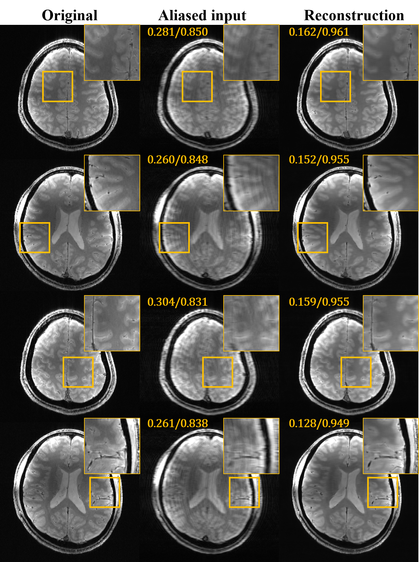
-C Application to 7T Data
We applied the propose algorithm to 7T images to demonstrate it applicability for high resolution images, as shown in Fig. 10. The 7T axial brain images were acquired in Cartesian coordinates from a 7T MR scanner (Philips, Achieva). A total of 567 images were scanned from nine subjects (63 slices per subject), with TR = 831 ms, TE = 5 ms, slice thickness = 0.75 mm, 292 292 acquisition matrix, 32 head coils, FOV = 240 240 mm, FA = 15∘, and lateral to lateral PE direction. Images from 7 subjects were used for training (441 images), 1 subject for validation (63 images), and the final subject for testing (63 images).
As with the previous studies above, we used uniform random sampling with 20% ACS lines, and the proposed algorithm significantly improved image quality and reduced aliasing artifacts.
References
- [1] K. P. Pruessmann, M. Weiger, M. B. Scheidegger, P. Boesiger et al., “SENSE: sensitivity encoding for fast MRI,” Magnetic resonance in medicine, vol. 42, no. 5, pp. 952–962, 1999.
- [2] M. A. Griswold, P. M. Jakob, R. M. Heidemann, M. Nittka, V. Jellus, J. Wang, B. Kiefer, and A. Haase, “Generalized autocalibrating partially parallel acquisitions (GRAPPA),” Magnetic resonance in medicine, vol. 47, no. 6, pp. 1202–1210, 2002.
- [3] D. L. Donoho, “Compressed sensing,” IEEE Transactions on information theory, vol. 52, no. 4, pp. 1289–1306, 2006.
- [4] M. Lustig, D. L. Donoho, J. M. Santos, and J. M. Pauly, “Compressed sensing MRI,” IEEE signal processing magazine, vol. 25, no. 2, pp. 72–82, 2008.
- [5] H. Jung, J. Ye, and E. Kim, “Improved k–t BLAST and k–t SENSE using FOCUSS,” Physics in Medicine and Biology, vol. 52, p. 3201, 2007.
- [6] H. Jung, K. Sung, K. Nayak, E. Kim, and J. Ye, “k-t FOCUSS: A general compressed sensing framework for high resolution dynamic MRI,” Magnetic Resonance in Medicine, vol. 61, no. 1, pp. 103–116, 2009.
- [7] P. J. Shin, P. E. Larson, M. A. Ohliger, M. Elad, J. M. Pauly, D. B. Vigneron, and M. Lustig, “Calibrationless parallel imaging reconstruction based on structured low-rank matrix completion,” Magn. Reson. Med., vol. 72, no. 4, pp. 959–970, 2014.
- [8] K. H. Jin, D. Lee, and J. C. Ye, “A general framework for compressed sensing and parallel MRI using annihilating filter based low-rank hankel matrix,” IEEE Trans. on Computational Imaging, vol. 2, no. 4, pp. 480–495, Dec 2016.
- [9] D. Lee, K. H. Jin, E. Y. Kim, S.-H. Park, and J. C. Ye, “Acceleration of MR parameter mapping using annihilating filter-based low rank hankel matrix (ALOHA),” Magnetic resonance in medicine, vol. 76, no. 6, p. 1848-1868, December 2016.
- [10] J. Lee, K. H. Jin, and J. C. Ye, “Reference-free single-pass EPI Nyquist ghost correction using annihilating filter-based low rank Hankel matrix (ALOHA),” Magnetic resonance in medicine, vol. 76, no. 8, p. 1775-1789, December 2016.
- [11] J. C. Ye, J. M. Kim, K. H. Jin, and K. Lee, “Compressive sampling using annihilating filter-based low-rank interpolation,” IEEE Transactions on Information Theory, vol. 63, no. 2, pp. 777–801, Feb. 2017.
- [12] A. Krizhevsky, I. Sutskever, and G. E. Hinton, “Imagenet classification with deep convolutional neural networks,” in Advances in Neural Information Processing Systems, 2012, pp. 1097–1105.
- [13] O. Ronneberger, P. Fischer, and T. Brox, “U-net: Convolutional networks for biomedical image segmentation,” in International Conference on Medical Image Computing and Computer-Assisted Intervention. Springer, 2015, pp. 234–241.
- [14] X.-J. Mao, C. Shen, and Y.-B. Yang, “Image denoising using very deep fully convolutional encoder-decoder networks with symmetric skip connections,” arXiv preprint, 2016.
- [15] K. Zhang, W. Zuo, Y. Chen, D. Meng, and L. Zhang, “Beyond a Gaussian denoiser: Residual learning of deep CNN for image denoising,” arXiv preprint arXiv:1608.03981, 2016.
- [16] C. Dong, C. C. Loy, K. He, and X. Tang, “Learning a deep convolutional network for image super-resolution,” in European Conference on Computer Vision. Springer, 2014, pp. 184–199.
- [17] J. Kim, J. Kwon Lee, and K. Mu Lee, “Accurate image super-resolution using very deep convolutional networks,” in Proceedings of the IEEE Conference on Computer Vision and Pattern Recognition, 2016, pp. 1646–1654.
- [18] C. Ledig, L. Theis, F. Huszár, J. Caballero, A. Cunningham, A. Acosta, A. Aitken, A. Tejani, J. Totz, Z. Wang et al., “Photo-realistic single image super-resolution using a generative adversarial network,” arXiv preprint, 2016.
- [19] S. Wang, Z. Su, L. Ying, X. Peng, S. Zhu, F. Liang, D. Feng, and D. Liang, “Accelerating magnetic resonance imaging via deep learning,” in 2016 IEEE 13th International Symposium on Biomedical Imaging (ISBI). IEEE, 2016, pp. 514–517.
- [20] K. Kwon, D. Kim, and H. Park, “A parallel MR imaging method using multilayer perceptron,” Medical Physics, 2017.
- [21] K. Hammernik, F. Knoll, D. Sodickson, and T. Pock, “Learning a variational model for compressed sensing MRI reconstruction,” in Proceedings of the International Society of Magnetic Resonance in Medicine (ISMRM), 2016.
- [22] E. Kang, J. Min, and J. C. Ye, “A deep convolutional neural network using directional wavelets for low-dose x-ray ct reconstruction,” Medical Physics, vol. 44, no. 10, 2017.
- [23] Y. Han, J. Yoo, and J. C. Ye, “Deep residual learning for compressed sensing CT reconstruction via persistent homology analysis,” arXiv preprint arXiv:1611.06391, 2016.
- [24] K. H. Jin, M. T. McCann, E. Froustey, and M. Unser, “Deep convolutional neural network for inverse problems in imaging,” IEEE Transactions on Image Processing, vol. 26, no. 9, pp. 4509–4522, 2017.
- [25] Y. Han, J. Yoo, and J. C. Ye, “Deep learning with domain adaptation for accelerated projection reconstruction MR,” Magnetic Resonance in Medicine (in press), available also as arXiv preprint arXiv:1703.01135, 2018.
- [26] K. He, X. Zhang, S. Ren, and J. Sun, “Deep residual learning for image recognition,” in Proceedings of the IEEE Conference on Computer Vision and Pattern Recognition, 2016, pp. 770–778.
- [27] J.-F. Cai, R. H. Chan, and Z. Shen, “A framelet-based image inpainting algorithm,” Applied and Computational Harmonic Analysis, vol. 24, no. 2, pp. 131–149, 2008.
- [28] J.-F. Cai, R. H. Chan, L. Shen, and Z. Shen, “Convergence analysis of tight framelet approach for missing data recovery,” Advances in Computational Mathematics, vol. 31, no. 1-3, pp. 87–113, 2009.
- [29] Y. Han and J. C. Ye, “Framing U-Net via deep convolutional framelets: Application to sparse-view CT,” arXiv preprint arXiv:1708.08333, 2017.
- [30] M. Lustig and J. M. Pauly, “SPIRiT: Iterative self-consistent parallel imaging reconstruction from arbitrary k-space,” Magnetic resonance in medicine, vol. 64, no. 2, pp. 457–471, 2010.
- [31] H. H. Bauschke and P. L. Combettes, Convex analysis and monotone operator theory in Hilbert spaces. Springer, 2011.
- [32] J. C. Ye, Y. Han, and E. Cha, “Deep convolutional framelets: A general deep learning framework for inverse problems,” SIAM Journal on Imaging Sciences (in press), also available as arXiv preprint arXiv:1707.00372, 2017.
- [33] J. Yoo, A. Wahab, and J. C. Ye, “A mathematical framework for deep learning in elastic source imaging,” arXiv preprint arXiv:1802.10055, 2018.
- [34] S. Ioffe and C. Szegedy, “Batch normalization: Accelerating deep network training by reducing internal covariate shift,” arXiv preprint arXiv:1502.03167, 2015.
- [35] P. J. Werbos, “Backpropagation through time: what it does and how to do it,” Proceedings of the IEEE, vol. 78, no. 10, pp. 1550–1560, 1990.
- [36] A. Vedaldi and K. Lenc, “Matconvnet: Convolutional neural networks for MATLAB,” in Proceedings of the 23rd ACM international conference on Multimedia. ACM, 2015, pp. 689–692.
- [37] X. Glorot and Y. Bengio, “Understanding the difficulty of training deep feedforward neural networks.” in Aistats, vol. 9, 2010, pp. 249–256.
- [38] Z. Wang, A. C. Bovik, H. R. Sheikh, and E. P. Simoncelli, “Image quality assessment: from error visibility to structural similarity,” IEEE Trans. on Image Processing, vol. 13, no. 4, pp. 600–612, 2004.
- [39] H. Zhao, O. Gallo, I. Frosio, and J. Kautz, “Is l2 a good loss function for neural networks for image processing?” ArXiv e-prints, vol. 1511, 2015.
- [40] D. Pathak, P. Krahenbuhl, J. Donahue, T. Darrell, and A. A. Efros, “Context encoders: Feature learning by inpainting,” in Proceedings of the IEEE Conference on Computer Vision and Pattern Recognition, 2016, pp. 2536–2544.
- [41] R. Zhang, P. Isola, and A. A. Efros, “Colorful image colorization,” in European Conference on Computer Vision. Springer, 2016, pp. 649–666.
- [42] I. Goodfellow, J. Pouget-Abadie, M. Mirza, B. Xu, D. Warde-Farley, S. Ozair, A. Courville, and Y. Bengio, “Generative adversarial nets,” in Advances in neural information processing systems, 2014, pp. 2672–2680.
- [43] M. Mardani, E. Gong, J. Y. Cheng, S. Vasanawala, G. Zaharchuk, M. Alley, N. Thakur, S. Han, W. Dally, J. M. Pauly et al., “Deep generative adversarial networks for compressed sensing automates MRI,” arXiv preprint arXiv:1706.00051, 2017.
- [44] Q. Yang, P. Yan, Y. Zhang, H. Yu, Y. Shi, X. Mou, M. K. Kalra, and G. Wang, “Low dose CT image denoising using a generative adversarial network with Wasserstein distance and perceptual loss,” arXiv preprint arXiv:1708.00961, 2017.
- [45] J. M. Wolterink, T. Leiner, M. A. Viergever, and I. Isgum, “Generative adversarial networks for noise reduction in low-dose CT,” IEEE Transactions on Medical Imaging, 2017.