Samsung Electronics
11email: {wonsik16.kim, bhavya.goyal, kunal.chawla, jm411.lee, keunjoo.kwon}@samsung.com
Attention-based Ensemble for
Deep Metric Learning
Abstract
Deep metric learning aims to learn an embedding function, modeled as deep neural network. This embedding function usually puts semantically similar images close while dissimilar images far from each other in the learned embedding space. Recently, ensemble has been applied to deep metric learning to yield state-of-the-art results. As one important aspect of ensemble, the learners should be diverse in their feature embeddings. To this end, we propose an attention-based ensemble, which uses multiple attention masks, so that each learner can attend to different parts of the object. We also propose a divergence loss, which encourages diversity among the learners. The proposed method is applied to the standard benchmarks of deep metric learning and experimental results show that it outperforms the state-of-the-art methods by a significant margin on image retrieval tasks.
Keywords:
attention, ensemble, deep metric learning1 Introduction
Deep metric learning has been actively researched recently. In deep metric learning, feature embedding function is modeled as a deep neural network. This feature embedding function embeds input images into feature embedding space with a certain desired condition. In this condition, the feature embeddings of similar images are required to be close to each other while those of dissimilar images are required to be far from each other. To satisfy this condition, many loss functions based on the distances between embeddings have been proposed [3, 6, 4, 37, 25, 29, 33, 27, 28, 14]. Deep metric learning has been successfully applied in image retrieval task on popular benchmarks such as CARS-196 [13], CUB-200-2011 [35], Stanford online products [29], and in-shop clothes retrieval [18] datasets.
Ensemble is a widely used technique of training multiple learners to get a combined model, which performs better than individual models. For deep metric learning, ensemble concatenates the feature embeddings learned by multiple learners which often leads to better embedding space under given constraints on the distances between image pairs. The keys to success in ensemble are high performance of individual learners as well as diversity among learners. To achieve this objective, different methods have been proposed [39, 22]. However, there has not been much research on optimal architecture to yield diversity of feature embeddings in deep metric learning.
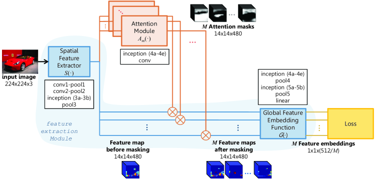
Our contribution is to propose a novel framework to encourage diversity in feature embeddings. To this end, we design an architecture which has multiple attention modules for multiple learners. By attending to different locations for different learners, diverse feature embedding functions are trained. They are regularized with divergence loss which aims to differentiate the feature embeddings from different learners. Equipped with it, we present -way attention-based ensemble (ABE-) which learns feature embedding with diverse attention masks. The proposed architecture is represented in Fig. 1(b). We compare our model to our -heads ensemble baseline [16], in which different feature embedding functions are trained for different learners (Fig. 1(a)), and experimentally demonstrate that the proposed ABE- shows significantly better results with less number of parameters.


2 Related works
2.0.1 Deep metric learning and ensemble
The aim of the deep metric learning is to find an embedding function which maps samples from a data space to a feature embedding space so that and are closer in some metric when and are semantically similar. To achieve this goal, in deep metric learning, contrastive [6, 4] and triplet [37, 25] losses are proposed. Recently, more advanced losses are introduced such as lifted structured loss [29], histogram loss [33], N-pair loss [27], and clustering loss [28, 14].
Recently, there has been research in networks incorporated with ensemble technique, which report better performances than those of single networks. Earlier deep learning approaches are based on direct averaging of the same networks with different initializations [15, 24] or training with different subsets of training samples [32, 31]. Following these former works, parameter sharing is introduced by Bachman et al. [2] which is called pseudo-ensembles. Another parameter sharing ensemble approach is proposed by Lee et al. [16]. Dropout [30] can be interpreted as an ensemble approach which takes exponential number of networks with high correlation. In addition to dropout, Veit et al. [34] state that residual networks behave like ensembles of relatively shallow networks. Recently the ensemble technique has been applied in deep metric learning as well. Yuan et al. [39] propose to ensemble a set of models with different complexities in cascaded manner. They train deeply supervised cascaded networks using easier examples through earlier layers of the networks while harder examples are further exploited in later layers. Opitz et al. [22] use online gradient boosting to train each learner in ensemble. They try to reduce correlation among learners using re-weighting of training samples. Opitz et al. [21] propose an efficient averaging strategy with a novel DivLoss which encourages diversity of individual learners.
2.0.2 Attention mechanism
Attention mechanism has been used in various computer vision problems. Earlier researches utilize RNN architectures for attention modeling [26, 19, 1]. These RNN based attention models solve classification tasks using object parts detection by sequentially selecting attention regions from images and then learning feature representations for each part. Besides RNN approaches, Liu et al. [17] propose fully convolutional attention networks, which adopts hard attention from a region generator. And Zhao et al. [40] propose diversified visual attention networks, which uses different scaling or cropping of input images for different attention masks. However, our ABE- is able to learn diverse attention masks without relying on a region generator. In addition, ABE- uses soft attention, therefore, the parameter update is straightforward by backpropagation in a fully gradient-based way while previous approaches in [26, 19, 1, 17, 40] use hard attention which requires policy gradient estimation.
Jaderberg et al. [11] propose spatial transformer networks which models attention mechanism using parameterized image transformations. Unlike aforementioned approaches, their model is differentiable and thus can be trained in a fully gradient-based way. However, their attention is limited to a set of predefined and parameterized transformations which could not yield arbitrary attention masks.
3 Attention-based ensemble
3.1 Deep metric learning
Let be an isometric embedding function between metric spaces and where is a dimensional metric space with an unknown metric function and is a dimensional metric space with a known metric function . For example, could be a Euclidean space with Euclidean distance or the unit sphere in a Euclidean space with angular distance.
Our goal is to approximate with a deep neural network from a dataset which are samples from . In case we cannot get the samples of metric , we consider the label information from the dataset with labels as the relative constraint of the metric . For example, from a dataset where is the set of labels, for the contrastive metric constraint could be defined as the following:
| (1) |
where is an arbitrary margin. The triplet metric constraint for could be defined as the following:
| (2) |
where is a margin. Note that these metric constraints are some choices of how to model , not those of how to model .
An embedding function is isometric or distance preserving embedding if for every one has . In order to have an isometric embedding function , we optimize so that the points embedded into produce exactly the same metric or obey the same metric constraint of .
3.2 Ensemble for deep metric learning
A classical ensemble for deep metric learning could be the method to average the metric of multiple embedding functions. We define the ensemble metric function for deep metric learning as the following:
| (3) |
where is an independently trained embedding function and we call it a learner.
In addition to the classical ensemble, we can consider the ensemble of two-step embedding function. Consider a function which is an isometric embedding function between metric spaces and where is a dimensional metric space with an unknown metric function and is a dimensional metric space with an unknown metric function . And we consider the isometric embedding where is a dimensional metric space with a known metric function . If we combine them into one function , the combined function is also an isometric embedding between metric spaces and .
Like the parameter sharing ensemble [16], with the independently trained multiple and a single , we can get multiple embedding functions as the following:
| (4) |
We are interested in another case where there are multiple embedding functions with multiple and a single as the following:
| (5) |
Note that a point in can be embedded into multiple points in by multiple learners. In Eq. (5), does not have to preserve the label information while it only has to preserve the metric. In other words, a point with a label could be mapped to multiple locations in by multiple and finally would be mapped to multiple locations in . If this were the ensemble of classification models where approximates the distribution of the labels, all should be label preserving functions because the outputs of become the inputs of one classification model .
For the embedding function of Eq. (5), we want to make attends to the diverse aspects of data in while maintaining a single embedding function which disentangles the complex manifold into Euclidean space. By exploiting the fact that a point in can be mapped to multiple locations in , we can encourage each to map into distinctive points in . Given an isometric embedding , if we enforce in mapped from to be far from each other, in mapped from will be far from each other as well. Note that we cannot apply this divergence constraint to because metric in is unknown. We train each to be isometric function between and while applying the divergence constraint among in . If we apply the divergence constraint to classical ensemble models or multihead ensemble models, they do not necessarily induce the diversity because each or could arbitrarily compose different metric spaces in (Refer to experimental results in Sec. 6.2). With the attention-based ensemble, union of metric spaces by multiple is mapped by a single embedding function .
3.3 Attention-based ensemble model

As one implementation of Eq.(5), we propose the attention-based ensemble model which is mainly composed of two parts: feature extraction module and attention module . For the feature extraction, we assume a general multi-layer perceptron model as the following:
| (6) |
We break it into two parts with a branching point at , includes , , and includes , , , . We call a spatial feature extractor and a global feature embedding function with respect to the output of each function. For attention module, we also assume a general multi-layer perceptron model which outputs a three dimensional blob with channel, width, and height as an attention mask. Each element in the attention masks is assumed to have a value from 0 to 1. Given aforementioned two modules, the combined embedding function for the learner is defined as the following:
| (7) |
where denotes element-wise product (Fig. 1(b)).
Note that, same feature extraction module is shared across different learners while individual learners have their own attention module . The attention function outputs an attention mask with same size as output of . This attention mask is applied to the output feature of with an element-wise product. Attended feature output of is then fed into global feature embedding function to generate an embedding feature vector. If all the elements in the attention mask are 1, the model is reduced to a conventional multi-layer perceptron model.
3.4 Loss
The loss for training aforementioned attention model is defined as:
| (8) |
where is a set of all training samples and labels, is the loss for the isometric embedding for the -th learner, is regularizing term for diversifying the feature embedding of each learner and is the weighting parameter to control the strength of the regularizer. More specifically, divergence loss is defined as the following:
| (9) |
where is set of all training samples, is the metric in and is a margin. A pair represents feature embeddings of a single image embedded by two different learners. We call it self pair from now on while positive and negative pairs refer to pairs of feature embeddings with same labels and different labels, respectively.
The divergence loss encourages each learner to attend to the different part of the input image by increasing the distance between the points embedded by the input image (Fig. 2). Since the learners share the same functional module to extract features, the only differentiating part is the attention module. Note that our proposed loss is not directly applied to the attention masks. In other words, the attention masks among the learners may overlap. And also it is possible to have the attention masks some of which focus on small region while other focus on larger region including small one.
4 Implementation
We perform all our experiments using GoogLeNet [32] as the base architecture. As shown in Fig. 3, we use the output of max pooling layer following the inception(3b) block as our spatial feature extractor and remaining network as our global feature embedding function . In our implementation, we simplify attention module as where consists of inception(4a) to inception(4e) from GoogLeNet, which is shared among all learners and consists of a convolution layer of 480 kernels of size 11 to match the output of for the element-wise product. This is for efficiency in terms of memory and computation time. Since is shared across different learners, forward and backward propagation time, memory usage, and number of parameters are decreased compared to having separate for each learner (without any shared part). Our preliminary experiments showed no performance drop with this choice of implementation.
We study the effects of different branching points and depth of attention module in Sec. 6.3. We use contrastive loss [6, 3, 4] as our distance metric loss function which is defined as the following:
| (10) | ||||
where is set of all training samples and corresponding labels, is the number of training sets, is a binary indicator of whether or not the label is equal to , is the euclidean distance, denotes the hinge function and is the margin for contrastive loss. Both of margins and (in Eq. 8) is set to 1.
We implement the proposed ABE- method using caffe [12] framework. During training, the network is initialized from a pre-trained network on ImageNet ILSVRC dataset [24]. The final layer of the network and the convolution layer of attention module are randomly initialized as proposed by Glorot et al. [5]. For optimizer, we use stochastic gradient descent with momentum optimizer with momentum as 0.9, and we select the base learning rate by tuning on validation set of the dataset.
We follow earlier works [29, 38] for preprocessing and unless stated otherwise, we use the input image size of 224224. All training and testing images are scaled such that their longer side is 256, keeping the aspect ratio fixed, and padding the shorter side to get 256256 images. During training, we randomly crop images to 224224 and then randomly flip horizontally. During testing, we use the center crop. We subtract the channel-wise mean of ImageNet dataset from the images. For training and testing images of cropped datasets, we follow the approach in [38]. For CARS-196 [13] cropped dataset, 256256 scaled cropped images are used; while for CUB-200-2011 [35] cropped dataset, 256256 scaled cropped images with fixed aspect ratio and shorter side padded are used.
We run our experiments on nVidia Tesla M40 GPU (24GBs GPU memory), which limits our batch size to 64 for ABE- model. Unless stated otherwise, we use the batch size of 64 for our experiments. We sample our mini-batches by first randomly sampling 32 images and then positive pairs for first 16 images and negative pairs for next 16 images, thus making the mini-batch of size 64. Unless mentioned otherwise, we report the results of our method using embedding size of 512. This makes the embedding size for individual learners to be 512/.
5 Evaluation
We use all commonly used image retrieval task datasets for our experiments and Recall@ metric for our evaluation. During testing, we compute the feature embeddings for all the test images from our network. For every test image, we then retrieve top similar images from the test set excluding test image itself. Recall score for that test image is 1 if at least one image out of retrieved images has the same label as the test image. We compute the average over whole test set to get Recall@. We evaluate the model after every 1000 iteration and report the results for the iteration with highest Recall@1.
We show the effectiveness of the proposed ABE- method on all the datasets commonly used in image retrieval tasks. We follow same train-test split as [29] for fair comparison with other works.
-
•
CARS-196 [13] dataset contains images of 196 different classes of cars and is primarily used for our experiments. The dataset is split into 8,144 training images and 8,041 testing images (98 classes in both).
-
•
CUB-200-2011 [35] dataset consists of 11,788 images of 200 different bird species. We use the first 100 classes for training (5,864 images) and the remaining 100 classes for testing (5,924 images).
-
•
Stanford online products (SOP) [29] dataset has 22,634 classes with 120,053 product images. 11,318 classes are used for training (59,551 images) while other 11,316 classes are for testing (60,502 images).
-
•
In-shop clothes retrieval [18] dataset contains 11,735 classes of clothing items with 54,642 images. Following similar protocol as [29], we use 3,997 classes for training (25,882 images) and other 3,985 classes for testing (28,760 images). The test set is partitioned into the query set of 3,985 classes (14,218 images) and the retrieval database set of 3,985 classes (12,612 images).
Since CARS-196 and CUB-200-2011 datasets consist of bounding boxes too, we report the results using original images and cropped images both for fair comparison.
6 Experiments
6.1 Comparison of ABE- with -heads
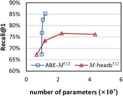
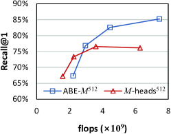
To show the effectiveness of our ABE- method, we first compare the performance of ABE- and -heads ensemble (Fig. 1(a)) with varying ensemble embedding sizes (denoted with superscript) on CARS-196 dataset. As show in Table 8 and Fig. 4, our method outperforms -heads ensemble by a significant margin. The number of model parameters for ABE- is much less compared to -heads ensemble as the global feature extractor is shared among learners. But, ABE- requires higher flops because of extra computation of attention modules. This difference becomes increasingly insignificant with increasing values of .
ABE-1 contains only one attention module and hence is not an ensemble and does not use divergence loss. ABE-1 performs similar to 1-head. We also report the performance of individual learners of the ensemble. From Table 8, we can see that the performance of ABE- ensemble is increasing with increasing . The performance of individual learners is also increasing with increasing despite the decrease in embedding size of individual learners (512/). The same increase is not seen for the case of -heads. Further, we can refer to ABE-164, ABE-2128, ABE-4256 and ABE-8512, where all individual learners have embedding size 64. We can see a clear increase in recall of individual learners with increasing values of .
| Ensemble | Individual Learners | params | flops | ||||||||
|---|---|---|---|---|---|---|---|---|---|---|---|
| 1 | 2 | 4 | 8 | 1 | 2 | 4 | 8 | () | () | ||
| 1-head512 | 67.2 | 77.4 | 85.3 | 90.7 | - | - | - | – | 0.65 | 1.58 | |
| 2-heads512 | 73.3 | 82.5 | 88.6 | 93.0 | 70.2.03 | 79.8.52 | 86.7.01 | 91.9.37 | 1.18 | 2.25 | |
| 4-heads512 | 76.6 | 84.2 | 89.3 | 93.2 | 70.4.80 | 79.9.38 | 86.5.43 | 91.4.42 | 2.24 | 3.60 | |
| 8-heads512 | 76.1 | 84.3 | 90.3 | 93.9 | 68.3.39 | 78.5.39 | 86.0.37 | 91.3.31 | 4.36 | 6.28 | |
| ABE-1512 | 67.3 | 77.3 | 85.3 | 90.9 | - | - | - | - | 0.97 | 2.21 | |
| ABE-2512 | 76.8 | 84.9 | 90.2 | 94.0 | 70.9.58 | 80.3.04 | 87.1.07 | 92.2.20 | 0.98 | 2.96 | |
| ABE-4512 | 82.5 | 89.1 | 93.0 | 95.5 | 74.4.51 | 83.1.47 | 89.1.34 | 93.2.36 | 1.05 | 4.46 | |
| ABE-8512 | 85.2 | 90.5 | 93.9 | 96.1 | 75.0.39 | 83.4.24 | 89.2.31 | 93.2.24 | 1.20 | 7.46 | |
| ABE-164 | 65.9 | 76.5 | 83.7 | 89.3 | - | - | - | - | 0.92 | 2.21 | |
| ABE-2128 | 75.5 | 84.0 | 89.4 | 93.6 | 68.6.38 | 78.8.38 | 85.7.43 | 91.3.16 | 0.96 | 2.96 | |
| ABE-4256 | 81.8 | 88.5 | 92.4 | 95.1 | 72.3.68 | 81.4.45 | 87.9.23 | 92.3.13 | 1.04 | 4.46 | |
6.2 Effects of divergence loss
6.2.1 ABE- without divergence loss
| Ensemble | Individual Learners | ||||||||||
|---|---|---|---|---|---|---|---|---|---|---|---|
| 1 | 2 | 4 | 8 | 1 | 2 | 4 | 8 | ||||
| ABE-8512 | 85.2 | 90.5 | 93.9 | 96.1 | 75.00.39 | 83.40.24 | 89.20.31 | 93.20.24 | |||
|
69.7 | 78.8 | 86.2 | 91.5 | 69.50.11 | 78.80.14 | 86.10.15 | 91.50.09 | |||
To analyze the effectiveness of divergence loss in ABE-, we conduct experiments without divergence loss on CARS-196 and show the results in Table 2. As we can see, ABE- without divergence loss performs similar to its individual learners whereas there is significant gain in ensemble performance of ABE- compared to its individual learners.
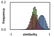
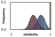
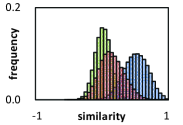
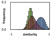
We also calculate the cosine similarity between positive, negative, and self pairs, and plot in Fig. 5. With divergence loss (Fig. 5), all learners learn diverse embedding function which leads to decrease in cosine similarity of self pairs. Without divergence loss (Fig. 5), all learners converge to very similar embedding function so that the cosine similarity of self pairs is close to 1. This could be because all learners end up learning similar attention masks which leads to similar embeddings for all of them.
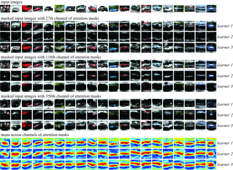
We visualize the learned attention masks of ABE-8 on CARS-196 in Fig. 6. Due to the space limitation, results from only three learners out of eight and three channels out of 480 are illustrated. The figure shows that different learners are attending to different parts for the same channel. Qualitatively, our proposed loss successfully diversify the attention masks produced by different learners. They are attending to different parts of the car such as upper part, bottom part, roof, tires, lights and so on. In 350th channel, for instance, learner 1 is focusing on bottom part of car, learner 2 on roof and learner 3 on upper part including roof. At the bottom of Fig. 6, the mean of the attention masks across all channels shows that the learned embedding function focuses more on object areas than the background.
6.2.2 Divergence loss in -heads
We show the result of experiments of 8-heads ensemble with divergence loss in Table 3. We can see that the divergence loss does not improve the performance in 8-heads. From Fig. 5, we can notice that cosine similarities of self pairs are close to zero for -heads. Fig. 5 shows that the divergence loss does not affect the cosine similarity of self pairs significantly. As mentioned in Sec. 3.2, we hypothesize this is because each of could arbitrarily compose different metric spaces in .
| 1 | 2 | 4 | 8 | |
|---|---|---|---|---|
| 8-heads | 76.1 | 84.3 | 90.3 | 93.9 |
| 8-heads with | 76.0 | 84.6 | 89.7 | 93.5 |
6.3 Ablation study
To analyze the importance of various aspects of our model, we performed experiments on CARS-196 dataset of ABE- model, varying a few hyperparameters at a time and keeping others fixed. (More ablation study can be found in the supplementary material.)
6.3.1 Sensitivity to depth of attention module
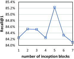
We demonstrate the effect of depth of attention module by changing the number of inception blocks in it. To make sure that we can take the element wise product of the attention mask with the input of attention module, the dimension of attention mask should match the input dimension of attention module. Because of this we remove all the pooling layers in our attention module. Fig. 7 shows Recall@1 with varying number of inception blocks in attention module starting from 1 (inception(4a)) to 7 (inception(4a) to inception(5b)) in GoogLeNet. We can see that the attention module with 5 inception blocks (inception(4a) to inception(4e)) performs the best.
6.3.2 Sensitivity to branching point of attention module
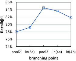
The branching point of the attention module is where we split the network between spatial feature extractor and global feature embedding function . To analyze the choice of branching point of the attention module, we keep the number of inception blocks in attention module same ( 5) and change branching points from pool2 to inception(4b). From Fig. 7, we see that pool3 performs the best with our architecture.
We carry out this experiment with batch size 40 for all the branching points. For ABE- model, the memory requirement for the is times compared to the individual learner. Since early branching point increases the depth of while decreasing the depth for , it would consequently increase the memory requirement of the whole network. Due to the memory constraints of GPU, we started the experiments from branching points pool2 and adjusted the batch size.
6.3.3 Sensitivity to
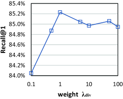
Fig. 7 shows the effect of on Recall@ for ABE- model. We can see that performs the best and lower values degrades the performance quickly.
6.4 Comparison with state of the art
We compare the results of our approach with current state-of-the-art techniques. Our model performs the best on all the major benchmarks for image retrieval. Table 4, 6 and 7 compare the results with previous methods such as LiftedStruct [29], HDC [39], Margin222All compared methods use GoogLeNet architecture except Margin which uses ResNet-50 [8] and Proxy-NCA uses IncpeptionBN [10] [38], BIER [22], and A-BIER [22] on CARS-196 [13], CUB-200-2011 [35], SOP [29], and in-shop clothes retrieval [18] datasets. Results on the cropped datasets are listed in Table 5.
| CUB-200-2011 | CARS-196 | ||||||||
| 1 | 2 | 4 | 8 | 1 | 2 | 4 | 8 | ||
| Contrastive128 [29] | 26.4 | 37.7 | 49.8 | 62.3 | 21.7 | 32.3 | 46.1 | 58.9 | |
| LiftedStruct128 [29] | 47.2 | 58.9 | 70.2 | 80.2 | 49.0 | 60.3 | 72.1 | 81.5 | |
| N-Pairs64 [27] | 51.0 | 63.3 | 74.3 | 83.2 | 71.1 | 79.7 | 86.5 | 91.6 | |
| Clustering64 [28] | 48.2 | 61.4 | 71.8 | 81.9 | 58.1 | 70.6 | 80.3 | 87.8 | |
| Proxy NCA264 [20] | 49.2 | 61.9 | 67.9 | 72.4 | 73.2 | 82.4 | 86.4 | 87.8 | |
| Smart Mining64 [7] | 49.8 | 62.3 | 74.1 | 83.3 | 64.7 | 76.2 | 84.2 | 90.2 | |
| Margin2128 [38] | 63.6 | 74.4 | 83.1 | 90.0 | 79.6 | 86.5 | 91.9 | 95.1 | |
| HDC384 [39] | 53.6 | 65.7 | 77.0 | 85.6 | 73.7 | 83.2 | 89.5 | 93.8 | |
| Angular Loss512 [36] | 54.7 | 66.3 | 76.0 | 83.9 | 71.4 | 81.4 | 87.5 | 92.1 | |
| A-Bier512 [23] | 57.5 | 68.7 | 78.3 | 86.2 | 82.0 | 89.0 | 93.2 | 96.1 | |
| ABE-2384 | 55.9 | 68.1 | 77.4 | 85.7 | 77.2 | 85.1 | 90.5 | 94.2 | |
| ABE-4384 | 57.8 | 69.0 | 78.8 | 86.5 | 82.2 | 88.6 | 92.6 | 95.6 | |
| ABE-8384 | 60.2 | 71.4 | 80.5 | 87.7 | 83.8 | 89.7 | 93.2 | 95.5 | |
| ABE-2512 | 55.7 | 67.9 | 78.3 | 85.5 | 76.8 | 84.9 | 90.2 | 94.0 | |
| ABE-4512 | 57.9 | 69.3 | 79.5 | 86.9 | 82.5 | 89.1 | 93.0 | 95.5 | |
| ABE-8512 | 60.6 | 71.5 | 79.8 | 87.4 | 85.2 | 90.5 | 94.0 | 96.1 | |
| CUB-200-2011 | CARS-196 | ||||||||
|---|---|---|---|---|---|---|---|---|---|
| 1 | 2 | 4 | 8 | 1 | 2 | 4 | 8 | ||
| PDDM + Triplet128 [9] | 50.9 | 62.1 | 73.2 | 82.5 | 46.4 | 58.2 | 70.3 | 80.1 | |
| PDDM + Quadruplet128 [9] | 58.3 | 69.2 | 79.0 | 88.4 | 57.4 | 68.6 | 80.1 | 89.4 | |
| HDC384 [39] | 60.7 | 72.4 | 81.9 | 89.2 | 83.8 | 89.8 | 93.6 | 96.2 | |
| Margin2128 [38] | 63.9 | 75.3 | 84.4 | 90.6 | 86.9 | 92.7 | 95.6 | 97.6 | |
| A-BIER512 [23] | 65.5 | 75.8 | 83.9 | 90.2 | 90.3 | 94.1 | 96.8 | 97.9 | |
| ABE-2512 | 64.9 | 76.2 | 84.2 | 90.0 | 88.2 | 92.8 | 95.6 | 97.3 | |
| ABE-4512 | 68.0 | 77.8 | 86.3 | 92.1 | 91.6 | 95.1 | 96.8 | 97.8 | |
| ABE-8512 | 70.6 | 79.8 | 86.9 | 92.2 | 93.0 | 95.9 | 97.5 | 98.5 | |
| 1 | 10 | 100 | 1000 | |
| Contrastive128 [29] | 42.0 | 58.2 | 73.8 | 89.1 |
| LiftedStruct512 [29] | 62.1 | 79.8 | 91.3 | 97.4 |
| N-Pairs512 [27] | 67.7 | 83.8 | 93.0 | 97.8 |
| Clustering64 [28] | 67.0 | 83.7 | 93.2 | - |
| Proxy NCA264 [20] | 73.7 | - | - | - |
| Margin2128 [38] | 72.7 | 86.2 | 93.8 | 98.0 |
| HDC384 [39] | 69.5 | 84.4 | 92.8 | 97.7 |
| A-Bier512 [23] | 74.2 | 86.9 | 94.0 | 97.8 |
| ABE-2512 | 75.4 | 88.0 | 94.7 | 98.2 |
| ABE-4512 | 75.9 | 88.3 | 94.8 | 98.2 |
| ABE-8512 | 76.3 | 88.4 | 94.8 | 98.2 |
| 1 | 10 | 20 | 30 | 40 | 50 | |
| FasionNet+Joints4096 [18] | 41.0 | 64.0 | 68.0 | 71.0 | 73.0 | 73.5 |
| FasionNet+Poselets4096 [18] | 42.0 | 65.0 | 70.0 | 72.0 | 72.0 | 75.0 |
| FasionNet4096 [18] | 53.0 | 73.0 | 76.0 | 77.0 | 79.0 | 80.0 |
| HDC384 [39] | 62.1 | 84.9 | 89.0 | 91.2 | 92.3 | 93.1 |
| A-BIER512 [23] | 83.1 | 95.1 | 96.9 | 97.5 | 97.8 | 98.0 |
| ABE-2512 | 85.2 | 96.0 | 97.2 | 97.8 | 98.2 | 98.4 |
| ABE-4512 | 86.7 | 96.4 | 97.6 | 98.0 | 98.4 | 98.6 |
| ABE-8512 | 87.3 | 96.7 | 97.9 | 98.2 | 98.5 | 98.7 |
7 Conclusion
In this work, we present a new framework for ensemble in the domain of deep metric learning. It uses attention-based architecture that attends to parts of the image. We use multiple such attention-based learners for our ensemble. Since ensemble benefits from diverse learners, we further introduce a divergence loss to diversify the feature embeddings learned by each learner. The divergence loss encourages that the attended parts of the image for each learner are different. Experimental results demonstrate that the divergence loss not only increases the performance of ensemble but also increases each individual learners’ performance compared to the baseline. We demonstrate that our method outperforms the current state-of-the-art techniques by significant margin on several image retrieval benchmarks including CARS-196 [13], CUB-200-2011 [35], SOP [29], and in-shop clothes retrieval [18] datasets.
References
- [1] Ba, J., Mnih, V., Kavukcuoglu, K.: Multiple object recognition with visual attention. In: International Conference on Learning Representations(2015)
- [2] Bachman, P., Alsharif, O., Precup, D.: Learning with pseudo-ensembles. In: Advances in Neural Information Processing Systems(2014)
- [3] Bell, S., Bala, K.: Learning visual similarity for product design with convolutional neural networks. Graphics 34(4), 98 (2015)
- [4] Chopra, S., Hadsell, R., LeCun, Y.: Learning a similarity metric discriminatively, with application to face verification. In: Computer Vision and Pattern Recognition(2005)
- [5] Glorot, X., Bengio, Y.: Understanding the difficulty of training deep feedforward neural networks. In: International Conference on Artificial Intelligence and Statistics (2010)
- [6] Hadsell, R., Chopra, S., LeCun, Y.: Dimensionality reduction by learning an invariant mapping. In: Computer Vision and Pattern Recognition(2006)
- [7] Harwood, B., VijayKumarB., G., Carneiro, G., Reid, I.D., Drummond, T.: Smart mining for deep metric learning. In: International Conference on Computer Vision(2017)
- [8] He, K., Zhang, X., Ren, S., Sun, J.: Deep residual learning for image recognition. In: Computer Vision and Pattern Recognition(2016)
- [9] Huang, C., Loy, C.C., Tang, X.: Local similarity-aware deep feature embedding. In: Advances in Neural Information Processing Systems(2016)
- [10] Ioffe, S., Szegedy, C.: Batch normalization: Accelerating deep network training by reducing internal covariate shift. In: International Conference on Machine Learning(2015)
- [11] Jaderberg, M., Simonyan, K., Zisserman, A., Kavukcuoglu, K.: Spatial transformer networks. In: Advances in Neural Information Processing Systems(2015)
- [12] Jia, Y., Shelhamer, E., Donahue, J., Karayev, S., Long, J., Girshick, R., Guadarrama, S., Darrell, T.: Caffe: Convolutional architecture for fast feature embedding. In: International Conference on Multimedia (2014)
- [13] Krause, J., Stark, M., Deng, J., Fei-Fei, L.: 3D object representations for fine-grained categorization. In: Workshop on 3D Representation and Recognition (2013)
- [14] Law, M.T., Urtasun, R., Zemel, R.S.: Deep spectral clustering learning. In: International Conference on Machine Learning(2017)
- [15] Lee, C.Y., Xie, S., Gallagher, P., Zhang, Z., Tu, Z.: Deeply-supervised nets. In: Artificial Intelligence and Statistics (2015)
- [16] Lee, S., Purushwalkam, S., Cogswell, M., Crandall, D., Batra, D.: Why M heads are better than one: Training a diverse ensemble of deep networks. arXiv preprint arXiv:1511.06314 (2015)
- [17] Liu, X., Xia, T., Wang, J., Lin, Y.: Fully convolutional attention localization networks: Efficient attention localization for fine-grained recognition. arXiv preprint arXiv:1603.06765 (2016)
- [18] Liu, Z., Luo, P., Qiu, S., Wang, X., Tang, X.: DeepFashion: Powering robust clothes recognition and retrieval with rich annotations. In: Computer Vision and Pattern Recognition(2016)
- [19] Mnih, V., Heess, N., Graves, A., et al.: Recurrent models of visual attention. In: Advances in Neural Information Processing Systems(2014)
- [20] Movshovitz-Attias, Y., Toshev, A., Leung, T.K., Ioffe, S., Singh, S.: No fuss distance metric learning using proxies. In: International Conference on Computer Vision(2017)
- [21] Opitz, M., Possegger, H., Bischof, H.: Efficient model averaging for deep neural networks. In: Asian Conference on Computer Vision(2016)
- [22] Opitz, M., Waltner, G., Possegger, H., Bischof, H.: BIER-boosting independent embeddings robustly. In: International Conference on Computer Vision(2017)
- [23] Opitz, M., Waltner, G., Possegger, H., Bischof, H.: Deep metric learning with BIER: Boosting independent embeddings robustly. arXiv preprint arXiv:1801.04815 (2018)
- [24] Russakovsky, O., Deng, J., Su, H., Krause, J., Satheesh, S., Ma, S., Huang, Z., Karpathy, A., Khosla, A., Bernstein, M., et al.: Imagenet large scale visual recognition challenge. International Journal of Computer Vision115(3), 211–252 (2015)
- [25] Schroff, F., Kalenichenko, D., Philbin, J.: Facenet: A unified embedding for face recognition and clustering. In: Computer Vision and Pattern Recognition(2015)
- [26] Sermanet, P., Frome, A., Real, E.: Attention for fine-grained categorization. In: International Conference on Learning Representationsworkshop (2015)
- [27] Sohn, K.: Improved deep metric learning with multi-class n-pair loss objective. In: Advances in Neural Information Processing Systems(2016)
- [28] Song, H.O., Jegelka, S., Rathod, V., Murphy, K.: Deep metric learning via facility location. In: Computer Vision and Pattern Recognition(2017)
- [29] Song, H.O., Xiang, Y., Jegelka, S., Savarese, S.: Deep metric learning via lifted structured feature embedding. In: Computer Vision and Pattern Recognition(2016)
- [30] Srivastava, N., Hinton, G., Krizhevsky, A., Sutskever, I., Salakhutdinov, R.: Dropout: A simple way to prevent neural networks from overfitting. Journal of Machine Learning Research 15(1), 1929–1958 (2014)
- [31] Sutskever, I., Vinyals, O., Le, Q.V.: Sequence to sequence learning with neural networks. In: Advances in Neural Information Processing Systems(2014)
- [32] Szegedy, C., Liu, W., Jia, Y., Sermanet, P., Reed, S., Anguelov, D., Erhan, D., Vanhoucke, V., Rabinovich, A.: Going deeper with convolutions. In: Computer Vision and Pattern Recognition(2015)
- [33] Ustinova, E., Lempitsky, V.: Learning deep embeddings with histogram loss. In: Advances in Neural Information Processing Systems(2016)
- [34] Veit, A., Wilber, M.J., Belongie, S.: Residual networks behave like ensembles of relatively shallow networks. In: Advances in Neural Information Processing Systems(2016)
- [35] Wah, C., Branson, S., Welinder, P., Perona, P., Belongie, S.: The Caltech-UCSD Birds-200-2011 Dataset. Tech. Rep. CNS-TR-2011-001, California Institute of Technology (2011)
- [36] Wang, J., Zhou, F., Wen, S., Liu, X., Lin, Y.: Deep metric learning with angular loss. In: International Conference on Computer Vision(2017)
- [37] Weinberger, K.Q., Saul, L.K.: Distance metric learning for large margin nearest neighbor classification. Journal of Machine Learning Research 10(2), 207–244 (2009)
- [38] Wu, C.Y., Manmatha, R., Smola, A.J., Krähenbühl, P.: Sampling matters in deep embedding learning. In: International Conference on Computer Vision(2017)
- [39] Yuan, Y., Yang, K., Zhang, C.: Hard-aware deeply cascaded embedding. In: International Conference on Computer Vision(2017)
- [40] Zhao, B., Wu, X., Feng, J., Peng, Q., Yan, S.: Diversified visual attention networks for fine-grained object classification. Multimedia 19(6), 1245–1256 (2017)
Attention-based Ensemble for Deep Metric Learning
(Supplementary Material)
Wonsik Kim, Bhavya Goyal, Kunal Chawla, Jungmin Lee, Keunjoo Kwon


In this supplementary material, we consider two additional architecutres for the ablation study: -heads+att and -tails. The details of each architectures are following. All experiments in this supplementary material are done on CARS-196 dataset. The models are trained with ensemble embedding size 512 and batch size 64, unless otherwise specified.
As described in Sec. 3 of the main manuscript, is the spatial feature extractor, is the global feature embedding function, and is the attention module. Our combined embedding function for the learner in ABE- is defined as the following:
| (11) |
where denotes element-wise product.
-
•
-heads+att It refers to the -heads with attention model, which is the ensemble of (Fig. 8(a)). Here, unlike our ABE- model, the global feature embedding function is not shared and the model is trained without divergence loss.
-
•
-tails Instead of having multiple heads and a shared tail, we can consider multiple tails and a shared head, which is (Fig. 8(b)). Unlike ABE-, there are no attention modules, and the spatial feature extractor is not shared, but the global feature embedding function is. It is also trained with divergence loss. Due to the memory constraint, this model is trained with a batch size of 32.
| Ensemble | Individual Learners | params | flops | ||||||||
|---|---|---|---|---|---|---|---|---|---|---|---|
| 1 | 2 | 4 | 8 | 1 | 2 | 4 | 8 | () | () | ||
| 8-heads | 76.1 | 84.3 | 90.3 | 93.9 | 68.3.39 | 78.5.39 | 86.0.37 | 91.3.31 | 4.36 | 6.28 | |
| 8-heads+att | 79.7 | 87.0 | 91.6 | 94.8 | 69.0.36 | 78.9.27 | 86.2.30 | 91.4.21 | 4.96 | 7.46 | |
| 8-tails | 81.1 | 88.0 | 92.4 | 95.4 | 71.4.83 | 80.9.55 | 87.5.31 | 92.3.26 | 1.08 | 12.7 | |
| ABE-8 | 85.2 | 90.5 | 93.9 | 96.1 | 75.0.39 | 83.4.24 | 89.2.31 | 93.2.24 | 1.20 | 7.46 | |
Table 8 summarizes the results. In addition, it also presents the results of -heads () and ABE- for comparison.
Effect of attention module on -heads
To study the contribution of attention module on performance, we propose -heads with attention model (-heads+att). This model has multiple heads and shared spatial feature extractor , like -heads model. In addition we attach different attention models for different learners, similar to our proposed ABE-. There are two differences between -heads+att and ABE-. Firstly, the global embedding function is not shared. Second, divergence loss is not applied during training. As discussed in the main manuscript, divergence loss is not required when the global embedding function is different for each learner.
The results show that with attention module, Recall@1 is improved from 76.1 to 79.7 compared to -heads. This comparison shows the effect of attention module independent from other factors. Along with the attention module, by sharing the global embedding function and applying divergence loss, ABE- further improves Recall@1 to 85.2.
Comparison of -heads and -tails
The main manuscript considers two different ways of ensembles in regards to two-step embedding function. In two-step embedding function, input is first mapped to an intermediate metric space by and then mapped to the final embedding space by . The first way of ensemble shares while having different for each learner. The second way shares while having different for each learner. To investigate the effect of two different ways of ensembles on performance, we propose -tails model as depicted in Fig. 8(a).
The results demonstrate -tails achieves better Recall@1 compared to -heads. The performance gain from this architecture (+5.0) is even larger than the case of -heads+att (+3.6). Compared to -tails, ABE- further improves the performance by using attention module.