Complexity of Leading Digit Sequences

Abstract

Let ${S_{a,b}}$ denote the sequence of leading digits of $a^{n}$ in base $b$. It is well known that if $a$ is not a rational power of $b$, then the sequence ${S_{a,b}}$ satisfies Benford’s Law; that is, digit $d$ occurs in ${S_{a,b}}$ with frequency $\log_{b}(1+1/d)$, for $d=1,2,\dots,b-1$.

In this paper, we investigate the complexity of such sequences. We focus mainly on the block complexity, $p_{a,b}(n)$, defined as the number of distinct blocks of length $n$ appearing in ${S_{a,b}}$. In our main result we determine $p_{a,b}(n)$ for all squarefree bases $b\geq 5$ and all rational numbers $a>0$ that are not integral powers of $b$. In particular, we show that, for all such pairs $(a,b)$, the complexity function $p_{a,b}(n)$ is an affine function, i.e., of the form $p_{a,b}(n)=c_{a,b}n+d_{a,b}$ for all $n\geq 1$, with coefficients $c_{a,b}\geq 1$ and $d_{a,b}\geq 0$, given explicitly in terms of $a$ and $b$. We also show that the requirement that $b$ be squarefree cannot be dropped: If $b$ is not squarefree, then there exist integers $a$ with $1<a<b$ for which $p_{a,b}(n)$ is not of the above form.

We use this result to obtain sharp upper and lower bounds for $p_{a,b}(n)$ and to determine the asymptotic behavior of this function as $b\to\infty$ through squarefree values. We also consider the question which affine functions $p(n)=cn+d$ arise as the complexity function $p_{a,b}(n)$ of some leading digit sequence ${S_{a,b}}$.

We conclude with a discussion of other complexity measures for the sequences ${S_{a,b}}$ and some open problems.

1 Introduction

1.1 Benford’s Law

The celebrated Benford’s Law, named after Frank Benford [Ben38], states that leading digits in many data sets tend to follow the Benford distribution, given by

$$P(d)=\log_{10}\left(1+\frac{1}{d}\right),\quad d=1,2,\dots,9.$$ (1.1)

Thus, in a data set following this distribution, approximately $\log_{10}2\approx 30.1\%$ of the numbers begin with digit $1$, approximately $\log_{10}(3/2)\approx 17.6\%$ begin with digit $2$, while only around $\log_{10}(10/9)\approx 4.6\%$ begin with digit $9$.

Benford’s Law has been found to be a good match for a wide range of real world data ranging from street addresses to populations of cities and accounting data, and it has become an important tool in detecting tax and accounting fraud. Several books on the topic have appeared in recent years (see, e.g., [BH15], [Mil15], [Nig12]), and nearly one thousand articles have been published (see [BHR17]).

In recent decades, there has been a growing body of literature investigating Benford’s Law for mathematical sequences. Benford’s Law has been shown to hold (in the sense of asymptotic density) for large classes of sequences, including exponentially growing sequences such as the powers of $2$ and the Fibonacci numbers, factorials, and the partition function; see, for example, Raimi [Rai76], Diaconis [Dia77], Hill [Hil95], Anderson et al. [ARS11], and Massé and Schneider [MS15].

While the global distribution and the global fit to Benford’s Law have been extensively investigated for large classes of arithmetic sequences and are now well understood, the local distribution of such sequences remains to a large extent unexplored, and more mysterious. Recent work (see [CFH⁺] and [CHL19]) revealed that most (but not all) of the classes of sequences that are known to satisfy Benford’s Law have poor local distribution properties, in the sense that $k$-tuples of leading digits of consecutive terms in the sequence do not behave like $k$ independent Benford-distributed random variables. This is illustrated in Table 1, which shows the leading digits (in base $10$) of the first $50$ terms of the sequences $\{a^{n}\}$, $a=2,\dots,9$. While the global distribution of digits in this table is roughly as predicted by Benford’s Law (for example, $30\%$ of the $400$ digits in the table are $1$), the local distribution is completely different: In some cases (e.g., for the sequence $\{2^{n}\}$) the leading digits seem to follow a near-periodic pattern, while in other cases (e.g., for the sequence $\{9^{n}\}$) they show excessive repetition in leading digits. In either case, there is a strong dependence of leading digits of consecutive terms of the sequence.

Sequence	Leading digits of first $50$ terms (concatenated)
$\{2^{n}\}$	2481361251 2481361251 2481361251 2481361251 2481371251
$\{3^{n}\}$	3928272615 1514141313 1392827262 6151514141 3139282727
$\{4^{n}\}$	4162141621 4162141621 4172141721 4172141731 4173141731
$\{5^{n}\}$	5216317319 4216317319 4215217319 4215217319 4215217318
$\{6^{n}\}$	6321742116 3217421163 2174211632 1742116321 8421163218
$\{7^{n}\}$	7432118542 1196432117 5321196432 1175321196 4321175321
$\{8^{n}\}$	8654322111 8654322111 9754332111 9765432211 1865432211
$\{9^{n}\}$	9876554433 3222211111 1987765544 3332222111 1119877655

Table 1: Leading digits (in base $10$) of the first $50$ terms of the sequences $\{a^{n}\}$, $a=2,\dots,9$.

Similar behavior can be found in more general sequences. For example, in [CHL19] it is shown that sequences of the form $\{2^{p(n)}\}$, where $p(n)$ is a polynomial, have excellent global, but poor local distribution properties with respect to Benford’s Law. On the other hand, numerical data obtained in [CFH⁺] suggests that the leading digits of the sequence $\{2^{p_{n}}\}$, where $p_{n}$ is the $n$-th prime, satisfy Benford’s Law on both the global and the local scale.

1.2 Complexity of sequences

In this paper we investigate leading digit sequences from the point of view of complexity. The “complexity” of a sequence $S=\{a_{n}\}$ over a finite set of symbols (for example, the digits $1,2,\dots,9$) can be measured in a variety of ways; see the surveys of Allouche [All12], Ferenczi [Fer99], and Kamae [Kam12] for an overview of different complexity measures. Here we will use as our primary complexity measure the block complexity defined as the function $p(n)=p_{S}(n)$ that counts the number of distinct “blocks” of length $n$ (i.e., $n$-tuples of consecutive terms) occurring in a sequence $S$.

The block complexity function $p_{S}(n)$ is the most commonly used complexity measure for arithmetical sequences $S$ and has been extensively studied. It is easy to see that the function $p_{S}(n)$ is bounded if and only if the sequence $S$ is eventually periodic. On the other hand, for random sequences, the block complexity function $p_{S}(n)$ grows at an exponential rate; more precisely, it satisfies $p_{S}(n)=k^{n}$, where $k$ is the number of distinct symbols in the sequence. In between these two extremes there is a rich spectrum of sequences with intermediate levels of complexity and corresponding rates of growth of $p_{S}(n)$. We refer to the papers cited above—in particular, Ferenczi [Fer99]—for further details, examples, and references.

1.3 The leading digit sequences ${S_{a,b}}$

Our main focus in this paper will be on leading digit sequences for geometrically growing sequences such as those shown in Table 1. More precisely, given an integer $b\geq 3$ and a real number $a>0$, we consider the sequence ${S_{a,b}}$ of leading digits of $a^{n}$ in base $b$; that is, ${S_{a,b}}$ is defined as

$${S_{a,b}}=\{D_{b}(a^{n})\}_{n=1}^{\infty},$$ (1.2)

where $D_{b}(x)$ denotes the leading digit of $x$ in base $b$, defined by

$$D_{b}(x)=d\Longleftrightarrow d\cdot b^{k}\leq x<(d+1)b^{k}\quad\text{for some $k\in\mathbb{Z}$}\quad(d=1,2,\dots,b-1).$$ (1.3)

We denote by $p_{a,b}(n)$ the associated (block) complexity function, i.e., the number of distinct blocks of length $n$ occurring in the sequence ${S_{a,b}}$. More formally, $p_{a,b}(n)$ is given by

$$p_{a,b}(n)=p_{{S_{a,b}}}(n)=\#\{(D_{b}(a^{m}),\dots,D_{b}(a^{m+n-1})):m=1,2,\dots\}.$$ (1.4)

The data in Table 1 suggests that the sequences ${S_{a,b}}$, while not being periodic, have low complexity. More extended computations confirm this: Figure 1 shows the behavior of the “empirical” complexity functions $p_{a,10}(n)$ for selected values of $a$ and $n\leq 100$, based on the first $100,000$ terms of the sequence.

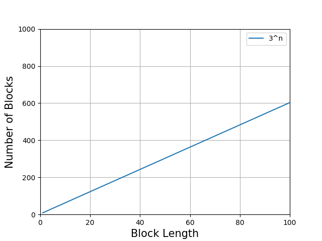
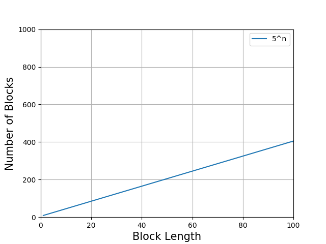
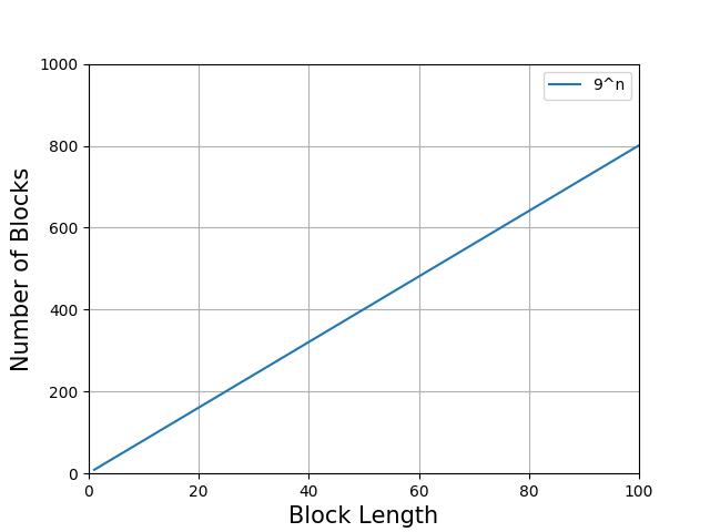
Figure 1: Empirical complexity functions for the leading digit sequences of $\{2^{n}\},\{3^{n}\},\{5^{n}\},\{9^{n}\}$ in base $10$, based on the first $100,000$ terms of these sequences.

The figure suggests that the functions $p_{a,10}(n)$ grow at a linear rate, with slopes depending on the value of $a$, though the precise nature of this dependence is unclear. Motivated by questions such as these, we seek to develop a complete understanding of the complexity of the sequences ${S_{a,b}}$.

1.4 Coding sequences of rotations

Given real numbers $\alpha>0$ and $x$ and a partition of the unit interval $0=\beta_{0}<\beta_{1}<\cdots<\beta_{p}=1$, the associated “coding sequence” $S=\{s_{n}\}$ is a sequence on $\{1,2,\dots,p\}$ defined by letting $s_{n}=k$ if and only if $\{n\alpha+x\}\in[\beta_{k-1},\beta_{k})$ (where $\{t\}=t-\lfloor t\rfloor$ denotes denotes the fractional part of $t$). Such sequences have been extensively studied in the literature; see, e.g., Alessandri and Berthé [AB98], and Berstel and Vuillon [BV02]. In particular, it is known (see, e.g., [AB98, Theorem 10]) that the complexity function of a coding sequence with irrational rotation $\alpha$ is ultimately affine, i.e., is of the form $p(n)=cn+d$ for sufficiently large $n$ (though in general not for all $n\geq 1$).

The leading digit sequences ${S_{a,b}}$ defined above can be viewed as a special type of coding sequence. To see this, note that (cf. Lemma 3.1 below) $a^{n}$ has leading digit $d$ in base $b$ if and only if $\{n\log_{b}a\}\in[\log_{b}d,\log_{b}(d+1))$, for $d=1,2,\dots,b-1$. Thus, ${S_{a,b}}$ is the coding sequence associated with the numbers $\alpha=\log_{b}a$ and $x=0$, and the partition $0=\log_{b}1<\log_{b}2<\dots<\log_{b}{(b-1)}<\log_{b}b=1$. It follows from the general result mentioned above that, if $\log_{b}a$ is irrational, then the complexity function $p_{a,b}(n)$ of ${S_{a,b}}$ is ultimately affine, i.e., of the form $cn+d$ for all sufficiently large $n$.

In this paper we will show that, when $a$ is rational, then, under some mild additional assumptions, the complexity function $p_{a,b}(n)$ is affine in the full sense, i.e., of the form $cn+d$ for all $n\geq 1$.

1.5 Summary of results and outline of paper

In Section 2 we state our main result, Theorem 2.2, which completely determines the complexity function $p_{a,b}(n)$ of the leading digit sequence ${S_{a,b}}$, for any squarefree base $b\geq 5$ and any positive rational number $a$ that is not an integral power of $b$. We show that, under these assumptions, $p_{a,b}(n)$ is an affine function, i.e., satisfies

$$p_{a,b}(n)=c_{a,b}n+d_{a,b},\quad n=1,2,3,\dots,$$ (1.5)

we give explicit formulas for the coefficients $c_{a,b}$ and $d_{a,b}$ in (1.5), and we derive several corollaries from this result.

To complement Theorem 2.2, we show in Theorem 2.3 and Corollary 2.4 that the requirement that $b$ be squarefree cannot be dropped: For any non-squarefree integer $b\geq 5$ there exists an integer $a$ with $1<a<b$ such that the complexity function $p_{a,b}(n)$ is not of the form (1.5) with $c_{a,b}\geq 1$.

In Section 3 we prove Theorems 2.2 and 2.3. Our approach uses results and techniques from the theory of dynamical systems generated by irrational “shifts” on the torus $\mathbb{T}$, along with some number-theoretic arguments.

In Section 4 we consider extreme values of the complexity function $p_{a,b}(n)$. We show that, under the above assumptions on $a$ and $b$, the complexity function $p_{a,b}(n)$ satisfies

$$\left\lfloor\frac{b-1}{2}\right\rfloor n+\left\lceil\frac{b-1}{2}\right\rceil\leq p_{a,b}(n)\leq(b-1)n,\quad n=1,2,\dots,$$

and that the upper and lower bounds are both sharp.

In Section 5 we determine the asymptotic behavior of the “slope” $c_{a,b}$ in (1.5) as $b\to\infty$ while $a$ is fixed. In particular, we show that if $a$ is an integer $\geq 2$, then the slope $c_{a,b}$ satisfies

$$c_{a,b}\sim\left(1-\frac{1}{a}\right)b$$

as $b\to\infty$ through squarefree values.

In Section 6 we consider the question which complexity functions $p(n)$ can be realized as the complexity function $p_{a,b}(n)$ of a leading digit sequence ${S_{a,b}}$ of the above type. By (1.5) such a complexity function is necessarily affine. However, not all affine functions $cn+d$ arise in this manner, and the question of which pairs $(c,d)$ of coefficients correspond to leading digit complexity functions leads to some interesting number-theoretic problems.

In Section 7 we consider another complexity measure, the “cyclomatic” complexity, which has been originally developed as a measure for the complexity of a graph and was adapted to the context of leading digit sequences by Iyengar et al. [IRU83] and Kak [Kak83]. We will determine the cyclomatic complexity for sequences of the form ${S_{a,b}}$.

In the final section, Section 8, we discuss some related work and present some open problems.

2 The complexity of ${S_{a,b}}$: Main results

2.1 Notations and conventions

We let $(n,m)$ denote the greatest common divisor of two integers $n$ and $m$. We denote by $\lfloor x\rfloor$ and $\lceil x\rceil$ the floor and ceiling functions, defined as the largest integer $\leq x$, resp. the smallest integer $\geq x$. We let $\{x\}=x-\lfloor x\rfloor$ denote the fractional part of $x$.

Throughout this paper we assume that $b$ is an integer $\geq 3$ and $a$ is a positive real number. For our main results we will restrict $b$ and $a$ further as follows:

Definition 2.1 (Admissible pairs).

A pair $(a,b)$ is called admissible if

• $b$ is a squarefree integer $\geq 5$; and

• $a$ is a positive rational number that is not an integral power of $b$.

Given an admissible pair $(a,b)$, we can represent the (rational) number $a$ uniquely in the form

$$a=\frac{r}{s}\,b^{k},\quad k\in\mathbb{Z},\quad r,s\in\mathbb{N},\quad(r,s)=1,\quad 1<\frac{r}{s}<b.$$ (2.1)

In particular, if $1<a<b$, then the integer $k$ in (2.1) is $0$, so the representation (2.1) reduces to $a=r/s$, the standard representation of $a$ as a reduced rational number.

2.2 Main result

We are now ready to state our main result, which completely describes the complexity function of ${S_{a,b}}$, for any admissible pair $(a,b)$.

Theorem 2.2 (Complexity of ${S_{a,b}}$: Main Result).

Let $(a,b)$ be an admissible pair and let $r$ and $s$ be defined by (2.1). Then the complexity function $p_{a,b}(n)$ of ${S_{a,b}}$ satisfies

$$p_{a,b}(n)=c_{a,b}n+d_{a,b},\quad n=1,2,\dots,$$ (2.2)

where

$$c_{a,b} =b-1-\left\lfloor\frac{b-1}{r}\right\rfloor-\left\lfloor\frac{(b,r)-1}{s}\right\rfloor,$$ (2.3)

$$d_{a,b} =b-1-c_{a,b}=\left\lfloor\frac{b-1}{r}\right\rfloor+\left\lfloor\frac{(b,r)-1}{s}\right\rfloor.$$ (2.4)

In particular, this result shows that $p_{a,b}(n)$ is an affine function for $n\geq 1$, with $c_{a,b}$ and $d_{a,b}$ representing, respectively, the slope and intercept of this function. Note that, by (2.4), $c_{a,b}$ and $d_{a,b}$ are related by the constraint $c_{a,b}+d_{a,b}=b-1$. Thus, the complexity function $p_{a,b}(n)$ is completely determined by either of the quantities $c_{a,b}$ and $d_{a,b}$ and the base $b$.

Table 2 gives a numerical illustration of the formulas of Theorem 2.2, showing the complexity functions for the leading digit sequences ${S_{a,b}}$ for $a=2,3,\dots,9$ and selected squarefree bases. In particular, the results for $b=10$ confirm the empirical observations made in Figure 1.

Sequence $\{a^{n}\}$	$\{2^{n}\}$	$\{3^{n}\}$	$\{4^{n}\}$	$\{5^{n}\}$	$\{6^{n}\}$	$\{7^{n}\}$	$\{8^{n}\}$	$\{9^{n}\}$
$b=5$	$2n+2$	$3n+1$	$3n+1$		$4n$	$4n$	$4n$	$4n$
$b=6$	$2n+3$	$2n+3$	$3n+2$	$4n+1$		$5n$	$4n+1$	$3n+2$
$b=7$	$3n+3$	$4n+2$	$5n+1$	$5n+1$	$5n+1$		$6n$	$6n$
$b=10$	$4n+5$	$6n+3$	$6n+3$	$4n+5$	$7n+2$	$8n+1$	$7n+2$	$8n+1$

Table 2: The complexity functions $p_{a,b}(n)$ for selected values of $a$ and $b$, computed using the formulas of Theorem 2.2. Blank entries correspond to pairs $(a,b)$ that are not admissible, i.e., cases where $a$ is an integral power of $b$.

It is natural to ask to what extent the restrictions imposed by the admissibility requirement can be relaxed. The following remarks address this question:

• The requirement that $a$ is not an integral power of $b$ serves to exclude trivial situations such as the sequence $\{10^{n}\}$ in base $10$. Indeed, it is not hard to see that whenever $a$ is a rational power of $b$, the sequence ${S_{a,b}}$ is periodic, and hence has a bounded complexity function. We remark that, under the additional assumptions (which are part of the admissibility condition) that $b$ is squarefree and $a$ is rational, the two conditions “$a$ is not an integral power of $b$” and “$a$ is not a rational power of $b$” are equivalent (cf. the proof of Corollary 3.3 below).

• We have stated our result only for rational values of $a$ as this is the most interesting, and most challenging, case. The result could be extended to irrational values of $a$, but complications arise in certain special cases, such as the sequence $\{(\sqrt{2})^{n}\}$. One can show that for all but countably many irrational numbers $a$ one has

  $$p_{a,b}(n)=(b-1)n,\quad n=1,2,\dots.$$

  In particular, $p_{a,b}(n)$ is of this form whenever $a$ is a transcendental number and $b$ an arbitrary integer $\geq 4$, not necessarily squarefree.

• The purpose of the restriction $b\geq 5$ is to avoid technical complications that arise in the case $b=3$ and which would require a separate treatment of this case. (These complications are due to the fact that, when $b=3$, the interval $[\log_{b}1,\log_{b}2)$ has length $>1/2$, whereas for $b\geq 4$ all intervals $[\log_{b}d,\log_{b}(d+1))$, $d=1,\dots,b-1$, have length $\leq 1/2$; cf. the footnote at the end of the proof of Lemma 3.4.)

• The most significant restriction in Theorem 2.2 is the requirement that the base $b$ be squarefree. The results below show that this restriction is, in a sense, best-possible. The restriction could, however, be replaced by other restrictions involving both $a$ and $b$. For example, we have $p_{a,b}(n)=(b-1)n$ for $n\geq 1$ whenever $a$ and $b$ are positive integers satisfying $a>b\geq 4$ and $(a,b)=1$.

Theorem 2.3 (Complexity of ${S_{a,b}}$: A counter-example).

Let $b\geq 5$ and $a\geq 2$ be integers such that $a^{2}$ is a divisor of $b$, and $b$ is not a rational power of $a$. Then

$$p_{a,b}(3)-p_{a,b}(2)\not=p_{a,b}(2)-p_{a,b}(1).$$ (2.5)

In particular, under the above assumptions on $a$ and $b$, the complexity function $p_{a,b}(n)$ is not affine for $n\geq 1$.

Corollary 2.4 (Failure of Theorem 2.2 for non-squarefree bases).

Given any non-squarefree integer $b\geq 5$, there exists an integer $a$ with $1<a<b$ such that $p_{a,b}(n)$ is not of the form

$$p_{a,b}(n)=cn+d,\quad n=1,2,\dots$$ (2.6)

for some integers $c\geq 1$ and $d$.

Proof.

Given a non-squarefree integer $b\geq 5$, let $q$ be a prime such that $q^{2}$ divides $b$, and take $a=q$. If $b$ is not a power of $q$, then Theorem 2.3 yields the desired conclusion. If $b$ is a power of $q$, say $b=q^{k}$ with $k\geq 2$, then the sequence ${S_{a,b}}$ of leading digits of $a^{n}(=q^{n})$ in base $b=q^{k}$ is the periodic sequence $q,q^{2},\dots,q^{k-1},1,q,q^{2},\dots,q^{k-1},1,q,q^{2},\dots$, and hence has bounded complexity function $p_{a,b}(n)$. In particular, (2.6) cannot hold with a positive coefficient $c$. ∎

We remark that, while for non-squarefree bases $b\geq 5$ and values of $a$ that are not rational powers of $b$, the complexity function $p_{a,b}(n)$ in general is not affine for all $n\geq 1$, the general results about codings of irrational rotations mentioned above (e.g., [AB98, Theorem 10]) imply that $p_{a,b}(n)$ is ultimately affine, i.e., is of the form $p_{a,b}(n)=cn+d$ for $n\geq n_{0}$, for suitable integers $n_{0}$, $c$ and $d$. However, determining explicit values of the coefficients $c$ and $d$ and thus obtaining a result analogous to Theorem 2.2 for non-squarefree values of $b$, seems to be a highly nontrivial task. (In particular, the formulas (2.3) and (2.4) are, in general, not valid when $b$ is not squarefree.)

2.3 Corollaries and special cases

Corollary 2.5 (Special Case: Integer Values $a$).

Let $b\geq 5$ be squarefree and let $a$ be a positive integer that is not an integral power of $b$. Then we have:

• If $1<a<b$, then

  $$p_{a,b}(n)=\left(b-\left\lfloor\frac{b-1}{a}\right\rfloor-(a,b)\right)n+\left\lfloor\frac{b-1}{a}\right\rfloor+(a,b)-1,\quad n=1,2,\dots$$ (2.7)

• If $a>b$ and $(a,b)=1$, then

  $$p_{a,b}(n)=(b-1)n,\quad n=1,2,\dots.$$ (2.8)

Proof.

The assumptions on $a$ and $b$ ensure that the pair $(a,b)$ is admissible, so we can apply the formulas of Theorem 2.2. Since $p_{a,b}(n)=c_{a,b}n+d_{a,b}$ and $d_{a,b}=b-1-c_{a,b}$ (see (2.4)), it suffices to show that

$$d_{a,b}=\begin{cases}\left\lfloor\frac{b-1}{a}\right\rfloor+(a,b)-1&\text{if $1<a<b$,}\\ 0&\text{if $a>b$ and $(a,b)=1$.}\end{cases}$$ (2.9)

Suppose first that $a$ is an integer satisfying $1<a<b$. Then in (2.1) we have $r=a$ and $s=1$. Hence the last term in (2.4) reduces to $(b,r)-1=(b,a)-1$, and (2.9) follows.

Now suppose that $a$ is an integer satisfying $a>b$ and $(a,b)=1$. Then in the representation (2.1) we have $r=a$ and $s=b^{k}$, where $k$ is such that $b^{k}<a<b^{k+1}$. Therefore $(b,r)=(b,a)=1$, and hence $\lfloor((b,r)-1)/s\rfloor=0$. Moreover, the assumption $a>b$ implies $\lfloor(b-1)/r\rfloor=\lfloor(b-1)/a\rfloor=0$. Hence both terms on the right of (2.4) are $0$, and we obtain $d_{a,b}=0$, as claimed. ∎

Example.

In base $b=10$, formula (2.7) gives $c_{a,10}=10-\lfloor 9/a\rfloor-(a,10)$ as the slope of the complexity function of $S_{a,10}$, Substituting $a=2,3,\dots,9$ in this formula yields the slopes $4,6,6,4,7,8,7,8$, respectively. By (2.4), the corresponding intercepts are given by $d_{a,10}=9-c_{a,10}$, so the associated complexity functions are $4n+5,6n+3,6n+3,4n+5,7n+2,8n+1,7n+2,8n+1$, respectively. These are the functions shown in the last row of Table 2.

Corollary 2.6 (Special Case: $a=2$).

Let $b$ be a squarefree integer $\geq 5$. Then the complexity function of the leading digit sequence of $2^{n}$ in base $b$ is given by

$$p_{2,b}(n)=\left\lfloor\frac{b-1}{2}\right\rfloor n+\left\lceil\frac{b-1}{2}\right\rceil,\quad n=1,2,\dots$$ (2.10)

Proof.

The requirement that $b$ is squarefree and $\geq 5$ ensures that $(2,b)$ is admissible. We can therefore apply Corollary 2.5 to get

$$c_{2,b}=b-\left\lfloor\frac{b-1}{2}\right\rfloor-(2,b).$$

If $b$ is even, this reduces to

$$c_{2,b}=b-\frac{b-2}{2}-2=\frac{b-2}{2}=\left\lfloor\frac{b-1}{2}\right\rfloor,$$

while for $b$ odd we get

$$c_{2,b}=b-\frac{b-1}{2}-1=\frac{b-1}{2}=\left\lfloor\frac{b-1}{2}\right\rfloor,$$

so in either case we have

$$c_{2,b}=\left\lfloor\frac{b-1}{2}\right\rfloor.$$

By the formulas (2.4) and (2.2), it follows that

$$d_{2,b}=b-1-c_{2,b}=b-1-\left\lfloor\frac{b-1}{2}\right\rfloor=\left\lceil\frac{b-1}{2}\right\rceil$$

and

$$p_{2,b}(n)=c_{2,b}n+d_{2,b}=\left\lfloor\frac{b-1}{2}\right\rfloor n+\left\lceil\frac{b-1}{2}\right\rceil,$$

as claimed. ∎

Corollary 2.7 (Symmetry Property).

Let $(a,b)$ be an admissible pair. Then $(b/a,b)$ is admissible and the sequences ${S_{a,b}}$ and $S_{b/a,b}$ have the same complexity function, i.e., we have

$$p_{a,b}(n)=p_{b/a,b}(n),\quad n=1,2,\dots$$ (2.11)

Example.

The symmetry property can be used to explain some (but not all) of the coincidences of complexity functions shown in Table 2. For example, in base $10$ the leading digit sequences of $\{2^{n}\}$ and $\{5^{n}\}$ both have complexity function $4n+5$. In base $6$, the leading digit sequences of $\{2^{n}\}$ and $\{3^{n}\}$ both have complexity function $2n+3$. Since $5=10/2$ and $3=6/2$, these relations follow from the symmetry property.

Proof.

First note that $a$ is an integral power of $b$ if and only if $b/a$ is an integral power of $b$. Thus $(a,b)$ is admissible if and only if $(b/a,b)$ is admissible. This proves the first assertion of the theorem.

Let $(a,b)$ be an admissible pair. To prove (2.11), it suffices to show that $d_{a,b}=d_{b/a,b}$, since this implies $c_{a,b}=c_{b/a,b}$ by the first identity in (2.4), and hence $p_{a,b}(n)=c_{a,b}n+d_{a,b}=p_{b/a,b}(n)$.

Replacing $a$ by $ab^{-k}$ with a suitable integer $k$ if necessary, we may assume that $a$ lies in the range $1<a<b$. Let $r/s$ be the representation of $a$ as a reduced rational number, as given by (2.1). Then (2.4) gives

$$d_{a,b}=\left\lfloor\frac{b-1}{r}\right\rfloor+\left\lfloor\frac{(b,r)-1}{s}\right\rfloor.$$ (2.12)

Now consider $a^{\prime}=b/a$, and let $r^{\prime}/s^{\prime}$ be the representation of $a^{\prime}$ as a reduced rational number. Since $1<a<b$ we have $1<a^{\prime}<b$, so formula (2.4) applies again with $r$ and $s$ replaced by $r^{\prime}$ and $s^{\prime}$, respectively, to give

$$d_{a^{\prime},b}=\left\lfloor\frac{b-1}{r^{\prime}}\right\rfloor+\left\lfloor\frac{(b,r^{\prime})-1}{s^{\prime}}\right\rfloor.$$ (2.13)

To prove the result, it suffices to show that the expressions on the right of (2.12) and (2.13) are equal.

Substituting $a=r/s$ into the definition of $a^{\prime}$ gives

$$a^{\prime}=\frac{b}{a}=\frac{bs}{r}=\frac{sb/(b,r)}{r/(b,r)}=\frac{sb_{1}}{r_{1}},$$ (2.14)

where

$$b_{1}=\frac{b}{(b,r)},\quad r_{1}=\frac{r}{(b,r)}.$$ (2.15)

Since $(b_{1},r_{1})=1$ and $(r,s)=1$, the numerator and denominator in the fraction on the right of (2.14) are coprime and hence must be equal to the quantities $r^{\prime}$ and $s^{\prime}$ in (2.13); that is, we have

$$r^{\prime}=sb_{1},\quad s^{\prime}=r_{1}.$$ (2.16)

It follows that

$$(b,r^{\prime})=(b,sb_{1})=b_{1}((b,r),s)=b_{1},$$ (2.17)

since $(r,s)=1$. Substituting (2.16) and (2.17) into (2.13), we get

$$d_{a^{\prime},b}=\left\lfloor\frac{b-1}{sb_{1}}\right\rfloor+\left\lfloor\frac{b_{1}-1}{r_{1}}\right\rfloor=\left\lfloor\frac{(b,r)-1/b_{1}}{s}\right\rfloor+\left\lfloor\frac{b_{1}-1}{r_{1}}\right\rfloor.$$ (2.18)

On the other hand, (2.12) can be written as

$$d_{a,b}=\left\lfloor\frac{b_{1}-1/(b,r)}{r_{1}}\right\rfloor+\left\lfloor\frac{(b,r)-1}{s}\right\rfloor.$$ (2.19)

Comparing (2.18) and (2.19), we see that the equality of these expressions will follow if we show that

$$\left\lfloor\frac{(b,r)-1/b_{1}}{s}\right\rfloor=\left\lfloor\frac{(b,r)-1}{s}\right\rfloor\text{\ and\ }\left\lfloor\frac{b_{1}-1/(b,r)}{r_{1}}\right\rfloor=\left\lfloor\frac{b_{1}-1}{r_{1}}\right\rfloor.$$

But this follows from the identity

$$\left\lfloor\frac{h-x}{k}\right\rfloor=\left\lfloor\frac{h-1}{k}\right\rfloor\quad(0<x\leq 1,\ h,k\in\mathbb{N}),$$

which holds since the open interval $((h-1)/k,h/k)$ does not contain an integer. ∎

3 Proof of Theorems 2.2 and 2.3

We begin with two known results that we will need in the course of the proof. We recall that $D_{b}(x)$ denotes the leading digit of $x$ in base $b$, as defined in (1.3), and that $\{t\}$ denotes the fractional part of $t$, defined as $\{t\}=t-\lfloor t\rfloor$. The following lemma relates $D_{b}(x)$ to the fractional part $\{\log_{b}x\}$. This connection is well-known in the literature on Benford’s Law (see, e.g., [Ben38] or [Dia77]).

Lemma 3.1 (Leading digit criterion).

Let $x$ be a positive real number and $b$ an integer $\geq 3$. Then for any digit $d\in\{1,2,\dots,b-1\}$ we have

$$D_{b}(x)=d\Longleftrightarrow\{\log_{b}x\}\in[\log_{b}d,\log_{b}(d+1)).$$ (3.1)

Proof.

By the definition of $D_{b}(x)$, we have

$$D_{b}(x)=d \Longleftrightarrow d\cdot b^{k}\leq x<(d+1)b^{k}\quad\text{for some $k\in\mathbb{Z}$}$$

$$\Longleftrightarrow\log_{b}d+k\leq\log_{b}x<\log_{b}(d+1)+k\quad\text{for some $k\in\mathbb{Z}$}$$

$$\Longleftrightarrow\log_{b}d\leq\{\log_{b}x\}<\log_{b}(d+1)$$

$$\Longleftrightarrow\{\log_{b}x\}\in[\log_{b}d,\log_{b}(d+1)),$$

where we used the fact that $0\leq\log_{b}d<\log_{b}(d+1)\leq 1$ for $1\leq d\leq b-1$. ∎

The following result is well-known; see, e.g., [HW79, Theorem 439].

Lemma 3.2.

Let $\alpha$ be an irrational number. Then the sequence $\{n\alpha\}$ is dense in the interval $[0,1)$.

Corollary 3.3.

If $(a,b)$ is an admissible pair, then the sequence $\{n\log_{b}a\}$ is dense in the interval $[0,1)$.

Proof.

Assume $(a,b)$ is an admissible pair. By Lemma 3.2 it suffices to show that, if $(a,b)$ is admissible, then $\log_{b}a$ is irrational, i.e., $a$ is not a rational power of $b$.

We argue by contradiction. Suppose $(a,b)$ is admissible and $a$ is a rational power of $b$, say $a=b^{p/q}$, where $p$ and $q$ are coprime positive integers. The admissibility condition implies that $a$ is a positive rational number, i.e., of the form $a=m/n$, where $m$ and $n$ are coprime positive integers, and that $b$ is squarefree, i.e., of the form $b=p_{1}\dots p_{k}$, where the $p_{i}$ are distinct primes. Substituting these representations into the relation $a=b^{p/q}$, we obtain $m/n=(p_{1}\dots p_{k})^{p/q}$, or equivalently $m^{q}=n^{q}p_{1}^{p}\dots p_{k}^{p}$.

Since $m$ and $n$ are coprime, this can only hold if $n=1$. Hence we must have $m^{q}=p_{1}^{p}\dots p_{k}^{p}$. By the Fundamental Theorem of Arithmetic it follows that $m$ must of the form $m=p_{1}^{\alpha_{1}}\dots p_{k}^{\alpha_{k}}$ with nonnegative integer exponents $\alpha_{i}$, and that $q\alpha_{i}=p$ for all $i$. This is only possible if $p/q=h$ is a positive integer and $\alpha_{i}=h$ for all $i$, i.e., if $m=(p_{1}\dots p_{k})^{h}=b^{h}$. But then $a=m/n=m=b^{h}$ is an integral power of $b$, contradicting the admissibility condition. This completes the proof. ∎

For the remainder of this section we fix an admissible pair $(a,b)$. Thus $b\geq 5$ is squarefree and $a$ is not an integral power of $b$. We remark that the assumption that $b$ is squarefree will only be needed in the latter part of the proof of Theorem 2.2 (beginning with Lemma 3.6); Lemmas 3.4 and 3.5 hold without this assumption.

Dividing $a$ by a power of $b$ if necessary, we may assume without loss of generality that $1<a<b$, so that $a=r/s$, where $r$ and $s$ are as in Theorem 2.2 (see (2.1)). The assumption $1<a<b$ then implies

$$1<\frac{r}{s}<b.$$ (3.2)

We introduce the following notations:

$$\alpha =\log_{b}a=\log_{b}\frac{r}{s},$$ (3.3)

$$D =\{1,2,\dots,b-1\},$$ (3.4)

$$L =\log_{b}D=\{\log_{b}1,\log_{b}2,\dots,\log_{b}(b-1)\},$$ (3.5)

$$L_{k} =\bigcup_{i=0}^{k-1}(L-i\alpha)=\{\log_{b}d-i\log_{b}a:d\in D,\ i=0,1,\dots,k-1\}.$$ (3.6)

We regard the sets $L_{k}$ as subsets of the one-dimensional torus $\mathbb{T}=\mathbb{R}/\mathbb{Z}$ by identifying elements that differ by an integer. The following key result relates the sets $L_{k}$ to the complexity functions that we seek to evaluate. More general results of this type are known in the context of codings of irrational rotations (see, e.g., [AB98, Theorem 10]). For the sake of completeness, we provide a self-contained proof here.

Lemma 3.4.

Let $p(k)=p_{a,b}(k)$ be the complexity function of the leading digit sequence ${S_{a,b}}$. Then

$$p(k)=|L_{k}|\quad(k=1,2,\dots),$$ (3.7)

where $|L_{k}|$ denotes the cardinality of $L_{k}$.

Proof.

Recall that $p(k)$ denotes the number of blocks of length $k$ in the sequence ${S_{a,b}}$, i.e., the number of distinct tuples $(d_{0},\dots,d_{k-1})$ of digits $d_{i}\in D$ such that, for some $n\in\mathbb{N}$,

$$D_{b}(a^{n+i})=d_{i},\quad i=0,1,\dots,k-1.$$ (3.8)

Using Lemma 3.1 we see that (recall that, by (3.3), $\alpha=\log_{b}a$)

$$D_{b}(a^{n+i})=d_{i} \Longleftrightarrow\{\log_{b}(a^{n+i})\}\in[\log_{b}d_{i},\log_{b}(d_{i}+1))$$

$$\Longleftrightarrow\{(n+i)\log_{b}a\}\in[\log_{b}d_{i},\log_{b}(d_{i}+1))$$

$$\Longleftrightarrow\{(n+i)\alpha\}\in[\log_{b}d_{i},\log_{b}(d_{i}+1))$$

$$\Longleftrightarrow n\alpha\in[\log_{b}d_{i}-i\alpha,\log_{b}(d_{i}+1)-i\alpha)+m_{i}\quad\text{for some $m_{i}\in\mathbb{Z}$.}$$

It follows that (3.8) holds if and only if

$$n\alpha\in\bigcap_{i=0}^{k-1}\Bigl{[}\log_{b}d_{i}-i\alpha+m_{i},\log_{b}(d_{i}+1)-i\alpha+m_{i}\Bigr{)}$$ (3.9)

for some $m_{0},\dots,m_{k-1}\in\mathbb{Z}$. Interpreting both sides of (3.9) as elements of $\mathbb{T}=\mathbb{R}/\mathbb{Z}$, we can rewrite this relation as

$$n\alpha\in\bigcap_{i=0}^{k-1}\Bigl{[}\log_{b}d_{i}-i\alpha,\log_{b}(d_{i}+1)-i\alpha\Bigr{)}\quad\text{in $\mathbb{T}$.}$$ (3.10)

Now, note that, by Corollary 3.3, the sequence $\{n\alpha\}$ is dense in the unit interval $[0,1)$. Thus, if the interval on the right of (3.10) is non-empty, it must contain an element of this sequence. Hence, given any $k$-tuple $(d_{0},\dots,d_{k-1})$ of digits in $D$ for which the interval on the right of (3.10) is non-empty, there exists an $n\in\mathbb{N}$ such that (3.8) holds for this tuple, i.e., the tuple $(d_{0},\dots,d_{k-1})$ occurs as a block of length $k$ in the sequence ${S_{a,b}}$. Conversely, if $(d_{0},\dots,d_{k-1})$ is a block of length $k$ occurring in ${S_{a,b}}$, then there exists an $n$ such that relation (3.10) holds, so the interval on the right of (3.10) must be non-empty.

It follows that the number of blocks of length $k$ in the sequence ${S_{a,b}}$ (and hence the value of the complexity function $p(k)$) is equal to the number of non-empty intervals in $\mathbb{T}$ generated on the right of (3.10) as each $d_{i}$ runs through the digits in $D=\{1,2,\dots,b-1\}$. But these intervals are exactly the intervals obtained by splitting up $\mathbb{T}$ at the points

$$\log_{b}d-i\alpha\in\mathbb{T},\quad d\in D,\quad i=0,1,\dots,k-1,$$ (3.11)

so the number of such intervals is equal to the number of distinct elements in (3.11). The latter elements form the elements of the set $L_{k}$, so the desired number is $|L_{k}|$. This completes the proof of Lemma 3.4. ∎

To complete the proof of Theorem 2.2, it remains to evaluate the numbers $|L_{k}|$. As mentioned, we consider the sets $L_{k}$ as subsets of $\mathbb{T}$. Thus, in what follows relations involving the elements of these sets are to be interpreted as relations among elements in $\mathbb{T}$, i.e., as relations that hold modulo $1$.

Lemma 3.5.

We have

$$|L_{1}| =b-1,$$ (3.12)

$$|L_{2}| =2(b-1)-\left\lfloor\frac{b-1}{r}\right\rfloor-\left\lfloor\frac{(b,r)-1}{s}\right\rfloor.$$ (3.13)

Proof.

By definition, $L_{1}$ is the set $L=\{\log_{b}1,\dots,\log_{b}(b-1)\}$, which has $b-1$ distinct elements in $\mathbb{T}$. Thus, $|L_{1}|=|L|=b-1$, proving (3.12).

Now consider $L_{2}$. By definition, $L_{2}=L\cup(L-\alpha)$. Thus,

$$|L_{2}|=|L|+|L-\alpha|-|L\cap(L-\alpha)|=2(b-1)-|L\cap(L-\alpha)|.$$

To prove (3.13), it therefore suffices to show

$$|L\cap(L-\alpha)|=\left\lfloor\frac{b-1}{r}\right\rfloor+\left\lfloor\frac{(b,r)-1}{s}\right\rfloor.$$ (3.14)

For the proof of (3.14), consider an element $x\in L\cap(L-\alpha)$. Since $x\in L$, $x$ must be of the form

$$x=\log_{b}d$$

for some $d\in D$, and since $0\leq\log_{b}1\leq\log_{b}d\leq\log_{b}(b-1)<1$, the digit $d$ is uniquely determined by $x$.

Similarly, since $x\in L-\alpha$, $x$ must also be of the form

$$x=\log_{b}d\,^{\prime}-\log_{b}a+m$$

for some $d\,^{\prime}\in D$ and $m\in\mathbb{Z}$. We therefore have

$$\log_{b}d=\log_{b}d\,^{\prime}-\log_{b}a+m,$$

or equivalently,

$$d=d\,^{\prime}a^{-1}b^{m}.$$

Since $a=r/s$, the latter relation can be written as

$$dr=d\,^{\prime}sb^{m}.$$ (3.15)

We next show that the integer $m$ in (3.15) (and hence also $d\,^{\prime}$) is uniquely determined by $d$ (and hence by $x$), and that $m$ must be either $0$ or $1$. Since $1/(b-1)\leq d/d\,^{\prime}\leq b-1$ and $1<r/s<b$ (see (3.2)), (3.15) implies

$$b^{m}=(d/d\,^{\prime})(r/s)<(b-1)b<b^{2}$$

and

$$b^{m}=(d/d\,^{\prime})(r/s)>\frac{1}{b-1}>\frac{1}{b},$$

so we have $-1<m<2$ and hence either $m=0$ or $m=1$. Moreover, for each given element $d\in D$ at most one of these cases can occur. Indeed, rewriting (3.15) as $d\,^{\prime}=d(r/s)b^{-m}$, we see that the integer $m$ (if it exists) is uniquely determined by the requirement that $1\leq d\,^{\prime}\leq b-1$.

Therefore we have

$$|L\cap(L-\alpha)|=N_{0}+N_{1},$$ (3.16)

where $N_{0}$ (resp. $N_{1}$) is the number of elements $d\in D$ satisfying (3.15) for some $d\,^{\prime}\in D$ with $m=0$ (resp. $m=1$). We will show that $N_{0}$ and $N_{1}$ are equal to the two terms on the right of (3.14).

Consider first the case $m=0$. Then (3.15) reduces to

$$dr=d\,^{\prime}s.$$ (3.17)

Since $r$ and $s$ are relatively prime, (3.17) can only hold if $d$ is a multiple of $s$ and $d\,^{\prime}$ is the same multiple of $r$, i.e., if $d=d_{0}s$ and $d\,^{\prime}=d_{0}r$ for some positive integer $d_{0}$. Furthermore, since $d\,^{\prime}\leq b-1$, we have

$$d_{0}=\frac{d\,^{\prime}}{r}\leq\frac{b-1}{r}.$$ (3.18)

We claim that each positive integer $d_{0}$ satisfying (3.18) yields a pair $(d,d\,^{\prime})$ of digits in $D$ for which (3.17) holds. Indeed, setting $d=d_{0}s$ and $d\,^{\prime}=d_{0}r$, we have $dr=d\,^{\prime}s$, and the bound $d_{0}\leq(b-1)/r$, along with our assumption $r/s>1$ (see (3.2)) imply that both $d$ and $d\,^{\prime}$ are positive integers bounded by $\leq b-1$ and hence are elements in $D$. Thus, the number of elements in the set $L\cap(L-\alpha)$ arising from case $m=0$ is equal to the number of positive integers $d_{0}$ satisfying (3.18), i.e., we have

$$N_{0}=\left\lfloor\frac{b-1}{r}\right\rfloor.$$ (3.19)

Now suppose that $m=1$. Then (3.15) reduces to

$$dr=d\,^{\prime}sb.$$ (3.20)

Set

$$b\,^{\prime}=\frac{b}{(b,r)},\quad r\,^{\prime}=\frac{r}{(b,r)}.$$

Dividing through by $(r,b)$, (3.20) becomes $dr\,^{\prime}=d\,^{\prime}sb\,^{\prime}$. Since $r\,^{\prime}$ is coprime with both $s$ and $b\,^{\prime}$, this can only hold if

$$d\,^{\prime}=d_{0}\kern-0.8pt^{\prime}r\,^{\prime}\quad\text{and}\quad d=d_{0}\kern-0.8pt^{\prime}sb\,^{\prime}$$

for some positive integer $d_{0}\kern-0.8pt^{\prime}$. Since $d\leq b-1$, the integer $d_{0}\kern-0.8pt^{\prime}$ must satisfy

$$d_{0}\kern-0.8pt^{\prime}\leq\frac{b-1}{sb\,^{\prime}}.$$ (3.21)

Conversely, every positive integer $d_{0}\kern-0.8pt^{\prime}$ satisfying (3.21) yields a pair $(d,d\,^{\prime})$ of digits in $D$ satisfying (3.20). Indeed, setting $d=d_{0}\kern-0.8pt^{\prime}sb\,^{\prime}$ and $d\,^{\prime}=d_{0}\kern-0.8pt^{\prime}r\,^{\prime}$, we have

$$dr=d(r,b)r\,^{\prime}=d_{0}\kern-0.8pt^{\prime}sb\,^{\prime}(r,b)r\,^{\prime}=d_{0}\kern-0.8pt^{\prime}r\,^{\prime}sb=d\,^{\prime}sb,$$

so (3.20) holds. Moreover, $d$ and $d\,^{\prime}$ are both positive integers and the bound (3.21) ensures that

$$d=d_{0}\kern-0.8pt^{\prime}sb\,^{\prime}\leq b-1$$

and

$$d\,^{\prime}=d_{0}\kern-0.8pt^{\prime}r\,^{\prime}\leq\frac{(b-1)}{sb\,^{\prime}}r\,^{\prime}=\frac{(b-1)(r/s)}{b}<b-1,$$

where in the last step we used the bound $r/s<b$. Thus the contribution of the case $m=1$ to the set $L\cap(L-\alpha)$ is equal to the number of positive integers $d_{0}\kern-0.8pt^{\prime}$ satisfying (3.21), i.e., we have

$$N_{1}=\left\lfloor\frac{b-1}{sb\,^{\prime}}\right\rfloor=\left\lfloor\frac{b}{sb\,^{\prime}}-\frac{1}{sb\,^{\prime}}\right\rfloor=\left\lfloor\frac{(b,r)-1/b\,^{\prime}}{s}\right\rfloor=\left\lfloor\frac{(b,r)-1}{s}\right\rfloor.$$ (3.22)

Substituting (3.19) and (3.22) into (3.16) yields the desired relation (3.14). ∎

Up to this point, our argument did not make use of the assumption that $b$ be squarefree. The following lemma, however, depends on this assumption in a crucial manner.

Lemma 3.6.

For any positive integer $k$ we have

$$|L_{k+1}|-|L_{k}|=|L_{2}|-|L_{1}|.$$ (3.23)

Proof.

By the definition of the sets $L_{k}$ we have

$$|L_{k+1}| =\left|\bigcup_{i=0}^{k}(L-i\alpha)\right|=\left|\bigcup_{i=1}^{k}(L-i\alpha)\right|+|L|-\left|L\cap\left(\bigcup_{i=1}^{k}(L-i\alpha)\right)\right|.$$

Since

$$\left|\bigcup_{i=1}^{k}(L-i\alpha)\right| =\left|\bigcup_{i=1}^{k}(L-i\alpha)+\alpha\right|=\left|\bigcup_{i=0}^{k-1}(L-i\alpha)\right|=|L_{k}|,$$

it follows that

$$|L_{k+1}|-|L_{k}|=|L|-\left|L\cap\left(\bigcup_{i=1}^{k}(L-i\alpha)\right)\right|.$$ (3.24)

Now note that for $k=1$ the right-hand side of (3.24) reduces to $|L|-|L\cap(L-\alpha)|$, whereas the left-hand side becomes $|L_{2}|-|L_{1}|$. Thus, to prove the desired relation (3.23), it suffices to show that

$$\left|L\cap\left(\bigcup_{i=1}^{k}(L-i\alpha)\right)\right|=\left|L\cap(L-\alpha)\right|.$$

This in turn will follow if we can show that, for any positive integer $i\geq 2$,

$$L\cap(L-i\alpha)\subset L\cap(L-\alpha).$$ (3.25)

It remains to prove (3.25). Fix $i\geq 2$, and consider an element $x\in L\cap(L-i\alpha)$. Since $x\in L$, $x$ must be of the form

$$x=\log_{b}d$$ (3.26)

for some $d\in D$. Since $x\in L-i\alpha$, $x$ must also be of the form

$$x=\log_{b}d\,^{\prime}-i\log_{b}a+m$$ (3.27)

for some $d\,^{\prime}\in D$ and $m\in\mathbb{Z}$. We need to show that $x\in L-\alpha$, i.e., that

$$x=\log_{b}d\,^{\prime\prime}-\log_{b}a+m\,^{\prime\prime}$$ (3.28)

for some $d\,^{\prime\prime}\in D$ and $m\,^{\prime\prime}\in\mathbb{Z}$.

From (3.26) and (3.27) we get

$$\log_{b}d=\log_{b}d\,^{\prime}-i\log_{b}a+m$$

and hence

$$d=d\,^{\prime}a^{-i}b^{m}.$$

Using $a=r/s$, this can be written as

$$dr^{i}=d\,^{\prime}b^{m}s^{i}.$$ (3.29)

On the other hand, by (3.26) the desired relation (3.28) is equivalent to

$$\log_{b}d=\log_{b}d\,^{\prime\prime}-\log_{b}a+m\,^{\prime\prime},$$

i.e.,

$$dr=d\,^{\prime\prime}b^{m\,^{\prime\prime}}s,$$ (3.30)

where $d\,^{\prime\prime}\in D$ and $m\,^{\prime\prime}\in\mathbb{Z}$. Thus, we seek to show that if (3.29) holds for some $d\,^{\prime}\in D$ and $m\in\mathbb{Z}$, then (3.30) holds for some $d\,^{\prime\prime}\in D$ and $m\,^{\prime\prime}\in\mathbb{Z}$.

Let

$$b_{0}=(b,r),\quad b\,^{\prime}=\frac{b}{b_{0}},\quad r\,^{\prime}=\frac{r}{b_{0}}.$$ (3.31)

By our assumption that $b$ is squarefree we have $(b\,^{\prime},b_{0})=1$ and since also $(b\,^{\prime},r\,^{\prime})=1$, it follows that

$$(b\,^{\prime},r)=(b\,^{\prime},r\,^{\prime}b_{0})=1.$$ (3.32)

Substituting $b=b_{0}b\,^{\prime}$ in (3.29), we obtain

$$d\,^{\prime}b_{0}^{m}b\,^{\prime}\,{}^{m}s^{i}=dr^{i}.$$ (3.33)

Now note that since $r/s>1$, (3.29) implies $b^{m}>(d/d\,^{\prime})\geq 1/(b-1)$, so the integer $m$ in (3.33) must satisfy $m\geq 0$. We consider the cases $m=0$ and $m\geq 1$ separately.

Suppose first that $m=0$. Then (3.33) reduces to

$$d\,^{\prime}s^{i}=dr^{i}.$$ (3.34)

Since $(s,r)=1$, it follows that $s^{i}$ divides $d$, i.e., we have

$$d=d_{0}s^{i}$$ (3.35)

for some positive integer $d_{0}$. Now let

$$d\,^{\prime\prime}=d(r/s).$$

Then $d\,^{\prime\prime}s=dr$, so (3.30) holds with $m\,^{\prime\prime}=0$. Moreover, by (3.35) we have

$$d\,^{\prime\prime}=d(r/s)=d_{0}s^{i}(r/s)=d_{0}rs^{i-1},$$

so $d\,^{\prime\prime}$ is a positive integer. In addition, $d\,^{\prime\prime}$ satisfies the upper bound

$$d\,^{\prime\prime}=d(r/s)\leq d(r/s)^{i}=d\,^{\prime}\leq b-1,$$

where we have used the inequality $r/s>1$ along with the relation (3.34). Thus, $d\,^{\prime\prime}$ is an element in $D$ satisfying (3.30) with $m\,^{\prime\prime}=0$. Thus we have reached the desired conclusion in the case $m=0$.

Now suppose that $m\geq 1$ in (3.33). Then $b\,^{\prime}s$ divides the left-hand side of (3.33), and hence also the right-hand side, i.e., $dr^{i}$. Since $(s,r)=1$ and $(b\,^{\prime},r)=1$ (see (3.32)), it follows that $b\,^{\prime}s$ divides $d$. Thus, we have

$$d=d_{0}\kern-0.8pt^{\prime}b\,^{\prime}s$$ (3.36)

for some positive integer $d_{0}\kern-0.8pt^{\prime}$. Let

$$d\,^{\prime\prime}=d_{0}\kern-0.8pt^{\prime}r\,^{\prime}.$$ (3.37)

Then, by (3.36),

$$d\,^{\prime\prime}bs=d_{0}\kern-0.8pt^{\prime}r\,^{\prime}bs=d_{0}\kern-0.8pt^{\prime}(r/b_{0})(b\,^{\prime}b_{0})s=(d_{0}\kern-0.8pt^{\prime}b\,^{\prime}s)r=dr,$$ (3.38)

so (3.30) holds with $m\,^{\prime\prime}=1$. Moreover, (3.37) shows that $d\,^{\prime\prime}$ is a positive integer, and by (3.38) and the bound $r/s<b$ (see (3.2)), $d\,^{\prime\prime}$ is bounded above by

$$d\,^{\prime\prime}\leq\frac{dr}{bs}<d\leq b-1.$$

Thus, $d\,^{\prime\prime}\in D$, and the proof of the lemma is complete. ∎

of Theorem 2.2.

We need to show that

$$p(k)=c_{a,b}k+d_{a,b},\quad k=1,2,\dots,$$ (3.39)

where

$$c_{a,b} =b-1-\left\lfloor\frac{b-1}{r}\right\rfloor-\left\lfloor\frac{(b,r)-1}{s}\right\rfloor,$$

$$d_{a,b} =b-1-c_{a,b}=\left\lfloor\frac{b-1}{r}\right\rfloor+\left\lfloor\frac{(b,r)-1}{s}\right\rfloor.$$

By Lemma 3.4 we have $p(k)=|L_{k}|$ for any positive integer $k$, so it suffices to show that (3.39) holds with $|L_{k}|$ in place of $p(k)$.

By the first part of Lemma 3.5 we have

$$|L_{1}|=b-1=c_{a,b}\cdot 1+d_{a,b},$$ (3.40)

so (3.39) holds for $k=1$. By the second part of Lemma 3.5 and Lemma 3.6 we have, for any $k\geq 2$,

$$|L_{k}| =|L_{1}|+\sum_{i=1}^{k-1}\left(|L_{i+1}|-|L_{i}|\right)$$

$$=|L_{1}|+(k-1)\left(|L_{2}|-|L_{1}|\right)$$

$$=c_{a,b}+d_{a,b}+(k-1)c_{a,b}=c_{a,b}k+d_{a,b},$$

which, combined with the relation $|L_{k}|=p(k)$, proves the desired formula (3.39). This completes the proof of Theorem 2.2. ∎

of Theorem 2.3.

Assume that $b\geq 5$ and $a\geq 2$ are integers such that $a^{2}$ divides $b$ and $b$ is not a rational power of $a$. We will show that in this case the complexity function $p(n)=p_{a,b}(n)$ satisfies $p(3)-p(2)\not=p(2)-p(1)$, and hence is not affine.

Since $a^{2}$ divides $b$ and $b$ is not a rational power of $a$, we have

$$b=a^{2}b_{1}$$ (3.41)

for some integer $b_{1}\geq 2$.

By Lemmas 3.4 and 3.5 (which, as noted above, do not depend on the assumption that $b$ is squarefree) it suffices to show

$$|L_{3}|-|L_{2}|\not=|L_{2}|-|L_{1}|.$$ (3.42)

Now, as in the proof of Lemma 3.6 (see (3.25)) we see that (3.42) is equivalent to

$$L\cap(L-2\alpha)\not\subset L\cap(L-\alpha).$$ (3.43)

Thus, it suffices to construct an element $x\in L$ such that $x\in L-2\alpha$, but $x\not\in L-\alpha$. (Recall that the sets $L$ are to be understood as subsets in $\mathbb{T}=\mathbb{R}/\mathbb{Z}$, so all relations are to be interpreted as relations that hold modulo $1$.).

We take

$$x=\log_{b}((a^{2}-1)b_{1})=\log_{b}\left(\frac{a^{2}-1}{a^{2}}b\right).$$ (3.44)

Then $x=\log_{b}d$, where $d=(a^{2}-1)b_{1}=b-b_{1}\in D$, so $x\in L$. Moreover, since $\alpha=\log_{b}a$, we have

$$x+2\alpha=\log_{b}\left(\frac{a^{2}-1}{a^{2}}b\right)+2\log_{b}a=\log_{b}(a^{2}-1)+1,$$

so $x=\log_{b}d\,^{\prime}-2\alpha+1$ with $d\,^{\prime}=a^{2}-1\in D$. Thus, $x\in L-2\alpha$ and hence $x\in L\cap(L-2\alpha)$.

On the other hand, we have

$$x+\alpha=\log_{b}\left(\frac{a^{2}-1}{a^{2}}b\right)+\log_{b}a=\log_{b}\left(\frac{a^{2}-1}{a}\right)+1,$$

and since $(a^{2}-1)/a$ is not an integer, but falls into the interval $1<(a^{2}-1)/a<b$, it follows that $x\not\in L-\alpha$. Thus, (3.43) holds, and the proof of Theorem 2.3 is complete. ∎

4 Extreme values of the complexity function $p_{a,b}(n)$

Theorem 4.1 (Extreme values of the complexity of ${S_{a,b}}$).

Let $(a,b)$ be an admissible pair. Then we have

$$\left\lfloor\frac{b-1}{2}\right\rfloor \leq c_{a,b}\leq b-1,$$ (4.1)

$$\left\lfloor\frac{b-1}{2}\right\rfloor n+\left\lceil\frac{b-1}{2}\right\rceil \leq p_{a,b}(n)\leq(b-1)n.$$ (4.2)

Moreover, the bounds in (4.1) and (4.2) are sharp: The upper bounds are attained for $a=b+1$, while the lower bounds are attained for $a=2$.

Proof.

First note that, by (2.4), we can write

$$p_{a,b}(n)=c_{a,b}n+(b-1)-c_{a,b}=(b-1)+c_{a,b}(n-1).$$

Thus, the maximal and minimal values of $p_{a,b}(n)$ are achieved when $c_{a,b}$ is maximal and minimal, respectively, and it therefore suffices to prove the bounds (4.1) for $c_{a,b}$.

The upper bound $c_{a,b}\leq b-1$ in (4.1) follows immediately from formula (2.3) of Theorem 2.2, and Corollary 2.5 shows that this bound is attained for $a=b+1$.

Now consider the lower bound in (4.1). When $a=2$, this bound follows from Corollary 2.6, which also shows that the bound is attained in this case. By the symmetry property (Corollary 2.7), the same conclusion holds for $a=b/2$.

We now consider the case when $a\not=2$ and $a\not=b/2$. Without loss of generality we may assume $1<a<b$, so that we have $a=r/s$ in the representation (2.1). Since, by the symmetry property, $p_{a,b}(n)=p_{b/a,b}(n)$, we may further restrict the range for $a$ to $1<a<\sqrt{b}$. (Note that we do not need to consider the case $a=\sqrt{b}$ since then the pair $(a,b)$ is not admissible.) Thus we have $a=r/s$, were $r$ and $s$ are positive integers satisfying

$$1<\frac{r}{s}<\sqrt{b},\quad(r,s)=1.$$ (4.3)

Note that, since $r/s>1$, we necessarily have $r\geq 2$. Moreover, the case $r=2$ can only occur when $s=1$, but this reduces to the case $a=r/s=2$ we considered above. Thus we may assume that $r\geq 3$. In this case, the bounds (4.3) imply

$$3\leq r<s\sqrt{b}.$$ (4.4)

By Theorem 2.2 we have

$$c_{a,b}=b-1-\left\lfloor\frac{b-1}{r}\right\rfloor-\left\lfloor\frac{(b,r)-1}{s}\right\rfloor.$$

Setting

$$f(r,s)=\left\lfloor\frac{b-1}{r}\right\rfloor+\left\lfloor\frac{(b,r)-1}{s}\right\rfloor,$$ (4.5)

the desired bound $c_{a,b}\geq\lfloor(b-1)/2\rfloor$ is seen to be equivalent to

$$f(r,s)\leq\left\lceil\frac{b-1}{2}\right\rceil.$$ (4.6)

To complete the proof of Theorem 4.1, it then remains to show that the inequality (4.6) holds whenever $r,s$ are positive integers satisfying (4.3) and (4.4).

We break the argument into several cases.

Case I: $r\geq b$. By (4.4), we have in this case $s>r/\sqrt{b}\geq\sqrt{b}$ and hence $s>2$. Therefore,

$$f(r,s)=\left\lfloor\frac{b-1}{r}\right\rfloor+\left\lfloor\frac{(b,r)-1}{s}\right\rfloor\leq\left\lfloor\frac{b-1}{b}\right\rfloor+\left\lfloor\frac{b-1}{2}\right\rfloor<\left\lceil\frac{b-1}{2}\right\rceil,$$ (4.7)

so the inequality (4.6) holds.

Case II: $b/3\leq r<b$, $b\geq 16$. First note that since $r<b$ we have $(b,r)\leq b/3$ unless $b$ is even and $r=b/2$. In the latter case, we may assume $s\geq 2$ since $s=1$ would reduce to the special case $a=r/s=b/2$ we considered earlier. Thus we have

$$\left\lfloor\frac{(b,r)-1}{s}\right\rfloor \leq\begin{cases}\left\lfloor\dfrac{b}{4}-\dfrac{1}{2}\right\rfloor&\text{if $b$ is even, $r=b/2$, $s\geq 2$,}\\[8.61108pt] \left\lfloor\dfrac{b}{3}-1\right\rfloor&\text{otherwise}\end{cases}$$

$$\leq\frac{b}{3}-\frac{1}{2}=\frac{b-1}{2}-\frac{b}{6}\leq\frac{b-1}{2}-\frac{8}{3},$$

where in the last step we used the assumption $b\geq 16$. Taking into account the lower bound $r\geq b/3$, we obtain

$$f(r,s) \leq\left\lfloor\frac{b-1}{b/3}\right\rfloor+\frac{b-1}{2}-\frac{8}{3}$$

$$=2+\frac{b-1}{2}-\frac{8}{3}<\left\lceil\frac{b-1}{2}\right\rceil.$$

Thus (4.6) holds in this case.

Case III: $3\leq r<b/3$, $b\geq 16$. We have

$$f(r,s)\leq\left\lfloor\frac{b-1}{r}\right\rfloor+(b,r)-1\leq\left\lfloor\frac{b-1}{r}+r-1\right\rfloor=\left\lfloor g(r)\right\rfloor,$$ (4.8)

say, where

$$g(r)=\frac{b-1}{r}+r-1.$$

Since $g^{\prime}(r)=-(b-1)r^{-2}+1$, the function $g(r)$ is decreasing in the range $3\leq r<\sqrt{b-1}$ and increasing in the range $r>\sqrt{b-1}$. Hence, the maximal value of this function on the interval $3\leq r\leq b/3$ occurs at one of the endpoints, $r=3$ and $r=b/3$. Now, since $b\geq 16$, we have

$$g(b/3) =\frac{b-1}{b/3}+\frac{b}{3}-1\leq 3+\frac{b}{3}-1=\frac{b-1}{2}-\frac{b-15}{6}<\frac{b-1}{2},$$

$$g(3) =\frac{b-1}{3}+2=\frac{b-1}{2}-\frac{b-1}{6}+2<\frac{b-1}{2},$$

since $b\geq 16$. Thus we have the bound

$$f(r,s)\leq\max(g(b/3),g(3))<\frac{b-1}{2}\leq\left\lceil\frac{b-1}{2}\right\rceil,$$ (4.9)

which proves (4.6) for Case III.

Case IV: $3\leq r<b$, $5\leq b\leq 15$. This case can be handled by direct computation of $f(r,s)$ for all pairs $(r,s)$ of positive integers satisfying (4.4) and comparing these values with $\lceil(b-1)/2\rceil$. ∎

5 Asymptotic and average behavior of the complexity function $p_{a,b}(n)$

In this section we consider two natural questions about the complexity of leading digit sequences ${S_{a,b}}$:

• Given a sequence $\{a^{n}\}$, how does the complexity of the associated leading digit sequence ${S_{a,b}}$ behave as the base $b$ tends to infinity?

• Given a base $b$, what can we say about the “average” complexity of the leading digit sequences ${S_{a,b}}$?

We will focus mainly on the case when $a$ is an integer. Figure 2 provides numerical data on these questions.

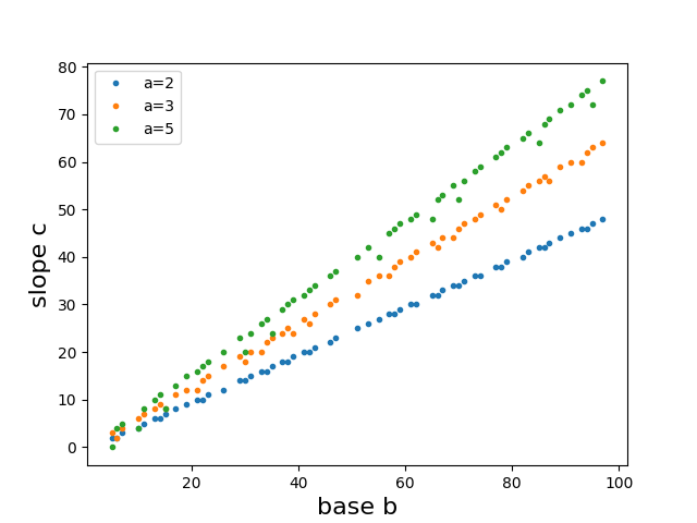
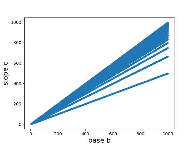
Figure 2: The figure on the left shows the slope $c=c_{a,b}$ of the complexity function of the leading digit sequence ${S_{a,b}}$, as a function of the base $b$ (restricted to squarefree values), for each of the values $a=2,3,5$. The figure on the right shows the set of all slopes $c_{a,b}$, as $a$ runs through integer values $2,3,\dots,b-1$. The values $c_{a,b}$ were computed using formula (2.3) of Theorem 2.2.

Figure 2 suggests that, as $b\to\infty$, the slope $c_{a,b}$ is asymptotically proportional to $b$, with the proportionality constant depending on the value $a$. In the following theorem we show that this is indeed the case and we determine the proportionality constant involved.

Theorem 5.1 (Asymptotic behavior of the complexity as $b\to\infty$).

Let $a$ be a fixed integer $\geq 2$, and suppose $b$ tends to infinity through squarefree values. Then we have

$$c_{a,b} =\left(1-\frac{1}{a}\right)b+O(1),$$ (5.1)

and, for any fixed integer $n\geq 1$,

$$p_{a,b}(n) =\left(1-\frac{1}{a}\right)nb+\frac{b}{a}+O(1).$$ (5.2)

Proof.

By part (i) of Corollary 2.5 we have

$$c_{a,b}=b-\left\lfloor\frac{b-1}{a}\right\rfloor-(a,b),$$

provided $b>a$ and $b$ is squarefree. Using the inequalities $1\leq(a,b)\leq a$ and $t-1\leq\lfloor t\rfloor\leq t$ it follows that

$$c_{a,b} \leq b-\frac{b-1}{a}+1-(a,b)\leq\left(1-\frac{1}{a}\right)b+\frac{1}{a},$$

$$c_{a,b} \geq b-\frac{b-1}{a}-(a,b)\geq\left(1-\frac{1}{a}\right)b-a,$$

which yields the first relation of the theorem, (5.1).

The second relation, (5.2), follows from the identity (see (2.2) and (2.4))

$$p_{a,b}(n)=c_{a,b}n+(b-1-c_{a,b}),$$ (5.3)

upon substituting the estimate (5.1) for $c_{a,b}$. ∎

We now turn to second question above, concerning the average behavior of the complexity function. In the theorem below we give an asymptotic estimate for the average slope of the complexity function $p_{a,b}(n)$, as $a$ runs through the $b-2$ integers $a=2,3,\dots,b-1$. Note that, if $b\geq 5$ is squarefree, then for each of these integers $(a,b)$ is admissible.

Let

$$\overline{c}_{b}=\frac{1}{b-2}\sum_{a=2}^{b-1}c_{a,b}.$$ (5.4)

be the average of the slopes $c_{a,b}$, taken over all integers $a$ in the interval $2\leq a\leq b-1$.

Theorem 5.2 (Average behavior of the complexity).

With the above notation we have, for any fixed $\epsilon>0$,

$$\overline{c}_{b}=b+O_{\epsilon}\left(b^{\epsilon}\right),$$ (5.5)

where the notation $O_{\epsilon}(\dots)$ means that the implied constant in the $O$-term depends on $\epsilon$.

Proof.

By part (i) of Corollary 2.5 we have

$$\sum_{a=2}^{b-1}c_{a,b} =\sum_{a=2}^{b-1}\left(b-\left\lfloor\frac{b-1}{a}\right\rfloor-(b,a)\right)=b(b-2)-\sum_{a=2}^{b-1}\left\lfloor\frac{b-1}{a}\right\rfloor-\sum_{a=2}^{b-1}(b,a).$$ (5.6)

Let $S_{1}$ and $S_{2}$ denote the last two sums. Then

$$S_{1}\leq\sum_{a=2}^{b-1}\frac{b-1}{a}=(b-1)(\log(b-1)+O(1))=O\left(b\log b\right).$$ (5.7)

Moreover,

$$S_{2} \leq\sum_{a=1}^{b}(a,b)\leq\sum_{d|b}d\,\#\{a\leq b-1:(a,b)=d\}$$ (5.8)

$$\leq\sum_{d|b}d\,\#\{a\leq b:d|a\}\leq\sum_{d|b}d\frac{b}{d}$$

$$=b\tau(b)=O_{\epsilon}\left(b^{1+\epsilon}\right),$$

where $\tau(b)$ denotes the number of divisors of $b$, and in the last step we have used the estimate (see, e.g., [HW79, Theorem 315])

$$\tau(b)=O_{\epsilon}\left(b^{\epsilon}\right),$$

which holds for any fixed $\epsilon>0$. Combining (5.6), (5.7), and (5.8), we get

$$\overline{c}_{b}=b+O_{\epsilon}(\log b)+O_{\epsilon}\left(b^{\epsilon}\right)=b+O_{\epsilon}\left(b^{\epsilon}\right),$$ (5.9)

as claimed. ∎

6 The set of complexity functions $p_{a,b}(n)$

A fundamental question in the complexity theory of sequences is which functions can arise as the complexity function $p_{S}(n)$ of some sequence $S$. There exists a large body of results in the literature establishing necessary or sufficient conditions on a complexity function; see Ferenczi [Fer99] for a survey. In particular, a result of Cassaigne [Cas97, Théorème 5.3] implies that any function of the form $cn+d$, where $c$ and $d$ are positive integers, is the complexity function of some sequence $S$ for all $n\geq 1$.

By Theorem 2.2, if $(a,b)$ is admissible, then the complexity function $p_{a,b}(n)$ of the leading digit sequence ${S_{a,b}}$ is necessarily an affine function, i.e., of the form $cn+d$. In light of the result mentioned above, the theorem therefore does not give rise to new classes of complexity functions. However, one can ask which functions $cn+d$ can be obtained as complexity functions of a sequence of the special form ${S_{a,b}}$. In this section we address this question. We begin with the following definition.

Definition 6.1 (Leading Digit Complexity Function and Good Pairs).

• A function $cn+d$ a called a leading digit complexity function if there exists an admissible pair $(a,b)$ such that $cn+d=p_{a,b}(n)$ for all $n$.

• A pair $(c,d)$ of integers is called good if it is the pair of coefficients of a leading digit complexity function $cn+d$.

We define the sets

$$G =\{(c,d):\text{ $cn+d$ is a leading digit complexity function}\},$$ (6.1)

$$G(c) =\{d:(c,d)\in G\}.$$ (6.2)

Thus, $G$ is the set of all “good” pairs $(c,d)$, and $|G(c)|$ is the number of good pairs with first coordinate $c$.

Figure 3 shows the behavior of $|G(c)|/\sqrt{c}$ as a function of $c$ and of $(\sum_{c\leq N}|G(c)|)N^{-3/2}$ as a function of $N$. The data suggests the first of these two functions is bounded above and below by positive constants, but does not converge to a limit, while the second function appears to converge to a limit.

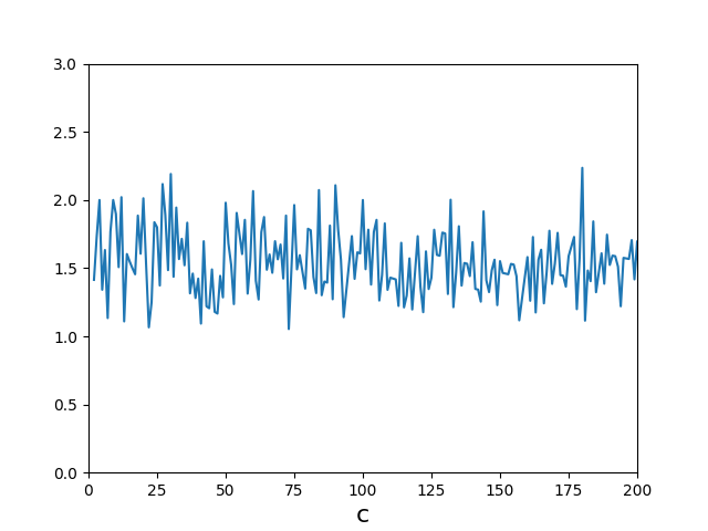
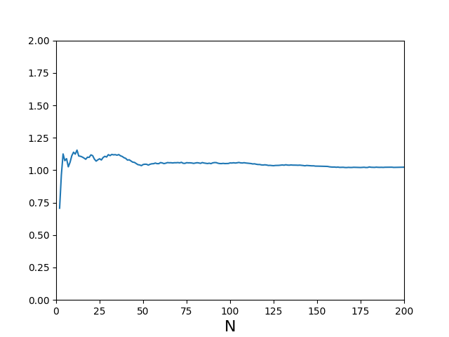
Figure 3: Number of good pairs $(c,d)$: The figure on the left shows the behavior of the function $|G(c)|/\sqrt{c}$ as a function of $c$. The figure on the right shows the behavior of $(\sum_{c\leq N}|G(c)|)N^{-3/2}$ as a function of $N$.

Motivated by such numerical data, we make the following conjecture:

Conjecture 6.2 (Number of Good Pairs).

• There exist positive constants $k_{1}$ and $k_{2}$ such that

  $$k_{1}\sqrt{c}\leq|G(c)|\leq k_{2}\sqrt{c}$$ (6.3)

  for all sufficiently large $c$, but the limit

  $$\lim_{c\to\infty}\frac{|G(c)|}{\sqrt{c}}$$ (6.4)

  does not exist.

• There exists a positive constant $k$ such that

  $$\sum_{c\leq N}|G(c)|\sim kN^{3/2}\quad(N\to\infty).$$ (6.5)

The numerical data presented in Figure 3 suggests that we can take $k_{1}=1$ and $k_{2}=2.5$ in (6.3). and $k=1$ in (6.5)

7 Other complexity measures

In a series of papers in the early 1980s (see [IRU83], [Kak83], [RUS⁺84]), S. Iyengar, A.K. Rajagopal, S.C. Kak and others studied the complexity of the sequence of leading digits of $2^{n}$ using graph-theoretic complexity measures. In this section, we describe this approach, and we determine explicitly the complexity of sequences ${S_{a,b}}$ with respect to a particular graph-theoretic complexity measure, the so-called cyclomatic complexity.

Cyclomatic complexity is a well-known complexity measure for graphs that is widely used as a measure for the complexity of computer programs.

Definition 7.1 (Cyclomatic Complexity of a Graph (McCabe [McC76], Berge [Ber73])).

Let $G$ be a finite directed graph. The cyclomatic complexity of $G$, $C_{G}$, is defined as

$$C_{G}=e-n+p,$$ (7.1)

where $e$ is the number of (directed) edges, $n$ the number of vertices, and $p$ the number of connected components of the graph $G$.

In order to apply this concept to the complexity of a sequence, one has to associate a graph to the sequence. Iyengar et al. [IRU83] suggest several ways to do so. The simplest, and most natural, approach is to consider the transition graph, $G_{S}$, of the sequence $S$, defined as the directed graph whose vertices are the symbols in $S$, and which contains an edge from $a$ to $b$ if and only if $a$ and $b$ occur in consecutive positions in the sequence $S$. We thus make the following definition.

Definition 7.2 (Cyclomatic Complexity of a Sequence $S$).

Let $S$ be an infinite sequence over a finite set of symbols, and let $G$ be its transition graph. The cyclomatic complexity, $C_{S}$, of the sequence $S$ is defined as the cyclomatic complexity of the transition graph $G$.

Under a mild additional assumption on $S$ (which amounts to a weak type of recurrence), we have the following connection between the cyclomatic complexity, $C_{S}$, of a sequence and its block complexity, $p_{S}(n)$.

Lemma 7.3 (Cyclomatic Complexity and Block Complexity).

Let $S$ be an infinite sequence over a finite set of symbols and assume that each symbol occurring in $S$ occurs infinitely often. Then we have

$$C_{S}=p_{S}(2)-p_{S}(1)+1.$$ (7.2)

Proof.

Let $G$ be the transition graph of $S$, and let $n$, $e$, and $p$ denote, respectively, the number of vertices, directed edges, and connected components of $G$.

The number of vertices in $G$ is the number of symbols in the sequence, which in turn is equal to the number of distinct blocks of length $1$ in the sequence, i.e., the quantity $p_{S}(1)$. Thus, we have

$$n=p_{S}(1).$$ (7.3)

Next, observe that there is a one-to-one correspondence between edges in $G$ and pairs $(d_{1},d_{2})$ of consecutive terms in the sequence ${S_{a,b}}$. Indeed, by the definition of the transition graph of a sequence, there is an edge from $d_{1}$ to $d_{2}$ if and only if $d_{1}$ and $d_{2}$ occur as consecutive terms in the sequence. Thus, the number of edges in $G$ is equal to the number of distinct pairs $(d_{1},d_{2})$ of consecutive terms in the sequence. But the latter number is the number of distinct blocks of length $2$ in the sequence, so we have

$$e=p_{S}(2).$$ (7.4)

Finally, we will show that the graph $G$ has only one connected component, i.e., that

$$p=1.$$ (7.5)

Indeed, by our assumption that each term $d$ that occurs in $S$ occurs there infinitely often, it follows that, given any two such terms, $d_{1}$ and $d_{2}$, the sequence must contain a string of consecutive terms beginning with $d_{1}$ and ending with $d_{2}$. By the definition of the transition graph $G$, this means that there is a path from $d_{1}$ to $d_{2}$. Since $d_{1}$ and $d_{2}$ were arbitrary terms (i.e., arbitrary vertices in $G$), it follows that the graph can have only one connected component, proving (7.5).

Substituting (7.3), (7.4), and (7.5) into (7.1), we obtain the desired relation (7.2). ∎

We now focus on the case of leading digit sequences of the form ${S_{a,b}}$, and we denote the cyclomatic complexity of such a sequence by $C_{a,b}$, i.e., we set $C_{a,b}=C_{S}$, where $S={S_{a,b}}$. Combining Lemma 7.3 with Theorem 2.2, we can determine $C_{a,b}$ explicitly for any for any admissible pair $(a,b)$:

Corollary 7.4 (Cyclomatic Complexity of ${S_{a,b}}$).

Let $(a,b)$ be an admissible pair, and let ${S_{a,b}}$ be the sequence of leading digits of $a^{n}$ in base $b$. Then the cyclomatic complexity of ${S_{a,b}}$ is given by

$$C_{a,b}=b-\left\lfloor\frac{b-1}{r}\right\rfloor-\left\lfloor\frac{(b,r)-1}{s}\right\rfloor,$$ (7.6)

where $r$ and $s$ are defined as in Theorem 2.2, i.e., as the unique integers satisfying

$$a=\frac{r}{s}\,b^{k},\quad k\in\mathbb{Z},\quad r,s\in\mathbb{N},\quad(r,s)=1,\quad 1<\frac{r}{s}<b.$$ (7.7)

Proof.

Let ${S_{a,b}}$ be as in the statement. It is easy to see (cf. the argument following (3.10)) that each digit $d\in\{1,2,\dots,b-1\}$ occurs infinitely often in ${S_{a,b}}$. Thus ${S_{a,b}}$ satisfies the hypothesis of Lemma 7.3, and hence has cyclomatic complexity given by $C_{a,b}=p_{a,b}(2)-p_{a,b}(1)+1$. Substituting the formulas (2.2) and (2.3) from Theorem 2.2, it follows that

$$C_{a,b}=c_{a,b}+1=b-\left\lfloor\frac{b-1}{r}\right\rfloor-\left\lfloor\frac{(b,r)-1}{s}\right\rfloor,$$

which is the desired formula (7.6). ∎

8 Concluding remarks

In this section we discuss some related concepts and open questions suggested by our results.

Rauzy graphs.

In Section 7 we defined the cyclomatic complexity of a sequence $S$ as the (graph-theoretic) cyclomatic complexity of the transition graph $G_{S}$ associated with this sequence. This transition graph is a particular case of a family of graphs associated with the sequence $S$, known as Rauzy graphs, and defined as follows: Given a sequence $S$, the Rauzy graph of level $n$, $\Gamma_{n}(S)$, is the directed graph whose vertices are the distinct “blocks” of length $n$ occurring in $S$, and in which two blocks of length $n$ are connected by a directed edge if and only if the second block “continues” the first block in the sense that it overlaps with the first block in its first $n-1$ positions; see Arnoux and Rauzy [AR91] and also Section 2.1 of [AB98].

The Rauzy graph $\Gamma_{1}(S)$ is the transition graph $G_{S}$ we have used to define the cyclomatic complexity of a sequence $S$. We remark that for sequences ${S_{a,b}}$ the cyclomatic complexity of the Rauzy graph $\Gamma_{n}({S_{a,b}})$ is independent of $n$: Indeed, the graph $\Gamma_{n}({S_{a,b}})$ has $p_{a,b}(n)$ vertices, $p_{a,b}(n+1)$ edges, and one connected component, so its cyclomatic complexity is $p_{a,b}(n+1)-p_{a,b}(n)+1=c_{a,b}+1$, where $c_{a,b}$ is the “slope” of $p_{a,b}(n)$, given by (2.3).

Another graph-theoretic complexity measure for sequences.

In their paper [IRU83], Iyengar et al. proposed an interesting graph-theoretic complexity measure for the leading digit sequence of $\{2^{n}\}$ that is different from the one we considered in the previous section. It is based on the remarkable fact, established in [IRU83], that the sequence of leading digits of $2^{n}$ can be completely decomposed into the five blocks $a=1248$, $b=1249$, $c=125$, $d=136$, and $e=137$. Rewriting the sequence as a sequence in the symbols $a,b,c,d,e$, one can then consider the associated transition graph between these symbols. This graph is different from the simple transition graph, and also from the general Rauzy graphs $\Gamma_{n}(S)$ considered above. Yet, as Iyengar et al. have shown, when $S$ is the leading digit sequence of $\{2^{n}\}$, all of these graphs have the same cyclomatic complexity, namely $5$.

Iyengar et al. focused mainly on the leading digit sequence of $\{2^{n}\}$. It would be interesting to see if their approach can be extended to the more general leading digit sequences ${S_{a,b}}$ we have considered in the present paper.

Complexity functions of other “natural” arithmetic sequences.

A key motivation for the present work was to completely determine the complexity function for a natural class of sequences of arithmetic interest, namely the sequences ${S_{a,b}}$ of leading digits of $a^{n}$ in base $b$. Another class of arithmetic sequences whose complexity has been analyzed in a similarly systematic manner are sequences obtained as expansions with respect to an irrational base $\beta>1$; see, e.g., Frougny et al. [FMP04] and Klouda and Pelantová [KP09].

As a natural extension of our results on the complexity of the sequences ${S_{a,b}}$, one can try to determine the complexity of more general leading digit sequences, such as the leading digits of $\{2^{n^{2}}\}$, $\{n!\}$, and $\{n^{n}\}$. Recent work [CHL19] on the local distribution of sequences of this type suggests that these sequences have relatively low complexity, possibly of polynomial rate of growth. On the other hand, in [CHL19] it was also shown that for “almost all” doubly exponential sequences $\{a^{\theta^{n}}\}$ the associated leading digit sequences behave locally like independent Benford-distributed random variables and thus have maximal complexity, i.e., satisfy $p(n)=9^{n}$ (in the case of base $10$). Interestingly, recent numerical investigations [CFH⁺] suggest that the same holds for the much slower growing sequence of Mersenne numbers $\{2^{p_{n}}-1\}$, where $p_{n}$ denotes the $n$-th prime number. Proving results of this type, however, seems to be well out of reach.