Improving Portfolios Global Performance with Robust Covariance Matrix Estimation:
Application to the Maximum Variety Portfolio

Abstract

This paper presents how the most recent improvements made on covariance matrix estimation and model order selection can be applied to the portfolio optimisation problem. The particular case of the Maximum Variety Portfolio is treated but the same improvements apply also in the other optimisation problems such as the Minimum Variance Portfolio. We assume that the most important information (or the latent factors) are embedded in correlated Elliptical Symmetric noise extending classical Gaussian assumptions. We propose here to focus on a recent method of model order selection allowing to efficiently estimate the subspace of main factors describing the market. This non-standard model order selection problem is solved through Random Matrix Theory and robust covariance matrix estimation. The proposed procedure will be explained through synthetic data and be applied and compared with standard techniques on real market data showing promising improvements.

I Introduction

Portfolio allocation is often associated with the mean-variance framework fathered by Markowitz in the 50’s [1]. This framework designs the allocation process as an optimisation problem where the portfolio weights are such that the expected return of the portfolio is maximised for a given level of portfolio risk. In practice this needs to estimate both expected returns and covariance matrix leading to estimation errors, particularly important for expected returns. This partly explains why many studies concentrate on allocation process relying solely on the covariance estimation such as the Global Minimum Variance Portfolio or the Equally Risk Contribution Portfolio [2], [3]. Another way to reduce the overall risk of a portfolio is to diversify the risks of its assets and to look for the assets weights that maximise a diversification indicator such as the variety (or diversification) ratio [4, 5], only involving the covariance matrix of the assets returns as well.
The frequently used covariance estimator is the Sample Covariance Matrix (SCM), optimal under the Normal assumption. Financial time series of returns might exhibit outliers related to abnormal returns leading to estimation errors larger than expected. The field of robust estimation [6], [7] intends to deal with this problem especially when $N$, the number of samples, is larger than $m$, the size of the observations vector. When $N<m$, the covariance matrix estimate is not invertible and regularization approaches are required. Some authors have proposed hybrid robust shrinkage covariance matrix estimates [8], [9], [10], building estimators upon Tyler’s robust M-estimator [6] and Ledoit-Wolf’s shrinkage approach [11].

Recent works [8], [12], [9], [13] based on Random Matrix Theory (RMT) have therefore considered robust estimation in the $m,N$ regime. In [13], the Global Minimum Variance Portfolio is studied and the authors show that applying an adapted estimation methodology based on the Shrinkage-Tyler M-estimator leads to achieving superior performance over may other competing methods. Another way to mitigate covariance matrix estimation errors is to filter the noisy part of the data. In financial applications, several empirical evidence militate in favour of the existence of multiple sources of risks challenging the CAPM single market factor assumption [14]. Whereas statistical methods like the principal component analysis may fail in distinguishing informative factors from the noisy ones, RMT helps in finding a solution for filtering noise [15, 16, 17, 18], even though the single market factor still prevails in the described cleaning method that is not completely satisfactory.
The application here proposes to mix several approaches: the assets returns are modelled as a multi-factor model embedded in correlated elliptical and symmetric noise and the final covariance estimate will be computed on the ”signal only” part of the observations, separable from the ”noise part” thanks to the results found in [19, 20, 21, 22].
The article is constructed as follows: section II presents the classical model and assumptions under consideration. Section III introduces the selected method of portfolio allocation for this paper: the Maximum Variety portfolio. Section IV explains how to solve the problem jointly with RMT and robust estimation theory which allow to design a consistent estimate of the number $K$ of informative factors. Section V shows some results obtained on experimental financial data highlighting the efficiency of the proposed method with regards to the conventional ones. Conclusion in section VI closes this paper.

&

Figure 1: Eigenvalue distributions. Left: SCM of observations. Middle: Tyler covariance matrix of observations. Right: Tyler covariance matrix of observations after whitening process. K-distributed case with shape parameter $\nu=0.5$, $\rho=0.8$, $m=100$, $N=1000$ ($c=0.1$), $K=3$, $\log(\bar{\lambda})=\log(1.7325)$.

Notations: Matrices are in bold and capital, vectors in bold. $Tr(\mathbf{X})$ is the trace of the matrix $\mathbf{X}$. $\left\|\mathbf{X}\right\|$ stands for the spectral norm. For any matrix $\mathbf{A}$, $\mathbf{A}^{T}$ is the transpose of $\mathbf{A}$. For any $m-$vector $\mathbf{x}$, $\mathcal{L}:\,\mathbf{x}\mapsto\mathcal{L}(\mathbf{x})$ is the $m\times m$ matrix defined as the Toeplitz operator: $\left([\mathcal{L}(\mathbf{x})]_{i,j}\right)_{i\leq j}=x_{i-j}$ and $\left([\mathcal{L}(\mathbf{x})]_{i,j}\right)_{i>j}=x_{i-j}^{\ast}$. For any matrix $\mathbf{A}$ of size $m\times m$, $\mathcal{T}(\mathbf{A})$ represents the matrix $\mathcal{L}(\check{\mathbf{a}})$ where $\check{\mathbf{a}}$ is a vector for which each component $\check{\mathbf{a}}_{i,\,0<i<m-1}$ contains the sum of the $i-$th diagonal of $\mathbf{A}$ divided by $m$.

II Model and assumptions

Suppose that our investment universe is composed of $m$ assets characterized at each time $t$ by their returns. Let’s denote by $\mathbf{R}=[\mathbf{r}_{1},\cdots,\mathbf{r}_{N}]$ the $m\times N$-matrix containing $N$ observations (or return $m$-vectors) $\{\mathbf{r}_{t}\}_{t\in[1,N]}$ at date $t$. We assume next that the returns of the $m$ assets can conjointly be expressed as a multi-factor model where an unknown number $K<m$ of factors may be characteristic of this universe (i.e. among the $m$ assets, there exists $K$ principal factors that are driving the universe comprising these particular $m$ assets). We assume the additive noise to be a multivariate Elliptical Symmetric noise [23, 24] generalizing a correlated multivariate non-Gaussian noise. We then have, for all $t\in[1,N]$: $\mathbf{r}_{t}=\mathbf{B}_{t}\,\mathbf{f}_{t}+\sqrt{\tau_{t}}\,\mathbf{C}^{1/2}\,\mathbf{x}_{t}$ where

• $\mathbf{r}_{t}$ is the $m$-vector of returns at time $t$,

• $\mathbf{B}_{t}$ is the $m\times K$-matrix of coefficients that define the sensitivity of the assets to each of the factor at time $t$,

• $\mathbf{f}_{t}$ is the K-vector of factor values at t, supposed to be common to all the assets,

• $\mathbf{x}_{t}$ is a zero-mean unitarily invariant random $m$-vector of norm $||\mathbf{x}_{t}||^{2}=1$,

• $\mathbf{C}$ is called the $m\times m$ scatter matrix (equal to the covariance matrix up to a constant) and is supposed to be Toeplitz structured and time invariant over the period of observation,

• $\tau_{t}$ is a real positive random variable at $t$ representing the variance of the noise. This quantity is different along the time $t$ and can efficiently pilot the non-Gaussian nature of the noise.

The efficient estimation of the number of factors $K$ is really a challenging problem for many financial applications:

• identifiability of the main $K$ factors to build new portfolios. This problem is for example closely related to linear unmixing problem in Hyperspectral Imaging [25],

• identifiability of the main $K$ factors to separate signal and noise subspaces in order to build projectors, to filter noisy part of the data through jointly robust and efficient covariance matrix estimation. This is for example useful for portfolio allocation or in risk management [26, 27, 28, 29].

The identified theoretical problem to solve is clearly the model order selection estimation as well as efficient method of covariance matrix estimation under correlated non-Gaussian noise hypothesis.

III Maximum Variety Portfolio

Portfolio allocation is a widely studied problem. Depending on the investment objective, the portfolio allocation differs. Apart from the well-known methods resides the differentiating Maximum Variety process that aims at maximising the Variety Ratio of the final portfolio. One way to quantify the degree of diversification of a portfolio invested in $m$ assets with proportions $\mathbf{w}=[w_{1},\ldots,w_{m}]^{T}$ is to compute the Variety Ratio of the portfolio:

$$VR(\mathbf{w},\boldsymbol{\Sigma})=\frac{\mathbf{w}^{T}\,\mathbf{s}}{\left(\mathbf{w}^{T}\,\boldsymbol{\Sigma}\,\mathbf{w}\right)^{1/2}}\,,\vspace{-0.1cm}$$ (1)

where $\mathbf{w}$ is the $m$-vector of weights, $w_{i}$ representing the allocation in asset $i$, $\boldsymbol{\Sigma}$ is the $m\times m$ covariance matrix of the $m$ assets returns and where $\mathbf{s}$ is the $m$-vector of the square roots of the diagonal element of $\boldsymbol{\Sigma}$, ie $s_{i}=\sqrt{\boldsymbol{\Sigma}_{ii}}$, representing the standard deviation of the returns of the $m$ assets. One way to allocate among the assets would be to maximise the above diversification ratio with respect to the weight vector $\mathbf{w}$ to obtain the solution $\mathbf{w}^{*}_{vr}$, also called the Maximum Diversified Portfolio in [4]:

$$\mathbf{w}^{*}_{vr}=\underset{\mathbf{w}}{\mathrm{argmin}}\,VR(\mathbf{w},\boldsymbol{\Sigma})\,,\vspace{-0.1cm}$$ (2)

under some conditions and constraints on the individual values of $\mathbf{w}$. In the following, we will impose only $0\leq w_{i}\leq 1$ $\forall i\in[1,m]$ and $\displaystyle\sum_{i=1}^{m}w_{i}=1$. As the objective function in (2) depends on the unknown covariance matrix $\boldsymbol{\Sigma}$, this latter has to be estimated in order to get the portfolio composition. This problem is one of the challenging problems in portfolio allocation and several methods can apply. The optimisation problem is shown to be very sensitive to outliers and to the chosen method of covariance matrix estimation. One of the main technique consists first in building a de-noised covariance matrix by thresholding the lowest eigenvalues and then in solving the objective function. The open questions always remain the choice of the covariance matrix estimate as well as the choice of the threshold value. To overcome these drawbacks and to answer these two questions, we propose a robust and quite simple technique based both on the class of the robust $M$-estimators and the RMT.

IV Proposed Methodology

Under general non-Gaussian noise hypothesis proposed in Section II, Tyler $M$-estimator [6, 30] is shown to be the most robust covariance matrix estimate. Given $N$ observations of the $m$-vector $\mathbf{r}_{t}$, the Tyler-$M$ estimate $\widehat{\mathbf{C}}_{tyl}$ is defined as the solution of the following ”fixed-point” equation:

$$\mathbf{C}=\displaystyle\frac{m}{N}\sum_{t=1}^{N}\frac{\mathbf{r}_{t}\,\mathbf{r}^{T}_{t}}{\mathbf{r}^{T}_{t}\,\mathbf{C}^{-1}\,\mathbf{r}_{t}},\vspace{-0.1cm}$$ (3)

with $Tr(\widehat{\mathbf{C}}_{tyl})=m$. The scatter matrix, solution of (3) has some remarquable properties [31, 32] like being robust and ”variance”-free and really reflects the true structure of the underlying process without power pollution. When the sources are present in the observations $\left\{\mathbf{r}_{t}\right\}$, the use of this estimator may lead to whiten the observations and to destroy the main information concentrated in the $K$ factors. When the noise is assumed white distributed, several methods, based on the RMT have been proposed [33] to extract information of interest from the received signals. One can cite for instance the number of embedded sources estimation [34], the problem of radar detection [35], signal subspace estimation [36]. However, when the additive noise is correlated, some RMT methods require the estimation of a specific threshold which has no explicit expression and can be very difficult to obtain [19, 37] while the others assume that the covariance matrix is known and use it, through some source-free secondary data, to whiten the signal. According to the following consistency theorem found and proved in [20, 21, 22], recent works have proposed to solve the problem through a biased Toeplitz estimate of $\widehat{\mathbf{C}}_{tyl}$, let’s say $\widetilde{\mathbf{C}}_{tyl}=\mathcal{T}\left(\widehat{\mathbf{C}}_{tyl}\right)$:

Consistency theorem.

Under the RMT regime assumption, ie that $N,m\rightarrow\infty$, and the ratio $c=m/N\rightarrow c>0$, we have the following spectral convergence:

$$\left\|\mathcal{T}\left(\widehat{\mathbf{C}}_{tyl}\right)-\mathbf{C}\right\|\stackrel{{\scriptstyle a.s.}}{{\longrightarrow}}0.$$ (4)

This powerful theorem says that it is possible to estimate the covariance matrix of the correlated noise even if the observations contain the sources or information to be retrieved. According to this result, the first step is then to whiten the observations using $\widetilde{\mathbf{C}}_{tyl}$. The whitened observations are defined as $\mathbf{r}_{w,t}=\widetilde{\mathbf{C}}_{tyl}^{-1/2}\,\mathbf{r}_{t}$. Given the set of $N$ whitened observations $\left\{\mathbf{r}_{w,t}\right\}$ and given the Tyler’s covariance matrix $\hat{\boldsymbol{\Sigma}}_{w}$ of these whitened returns, recent work [22] has shown that this whitening process allows us to consider that the eigenvalues distribution of $\boldsymbol{\Sigma}_{w}$ has to fit the predicted bounded distribution of Marčenko-Pastur [38] except for a finite number of eigenvalues if any source is still present and powerful enough to be detected outside the upper bound of the Marčenko-Pastur distribution given by $\bar{\lambda}=\left(1+\sqrt{c}\right)^{2}$. Figure I compares the eigenvalues distribution of the SCM $\hat{\mathbf{C}}_{scm}=\mathbf{R}\,\mathbf{R}^{T}/N$, $\hat{\mathbf{C}}_{tyl}$ and $\hat{\boldsymbol{\Sigma}}_{w}$ for $K=3$ sources of information embedded in non-Gaussian correlated K-distributed noise. If no whitening operation is made before applying the Marčenko-Pastur boundary properties of the eigenvalues, then there is no chance to detect any of the sources. After whitening process, the only detected sources above the Marčenko-Pastur threshold correspond to the $K$ sources. As a matter of fact, there is no need anymore to adapt the value of the threshold value regarding the distribution of $\tau_{t}$ and the estimated value of $\mbox{IE}[\tau]$ [22]. The robust Tyler $M$-estimator is ”$\tau$-free”, i.e. it does not depend anymore of the distribution of $\tau_{t}$. Once the $K$ largest eigenvalues larger than $\bar{\lambda}$ are detected, we set the $m-K$ lowest ones to $\left(Tr\left(\hat{\boldsymbol{\Sigma}}_{w}\right)-\sum_{k=K+1}^{m}\lambda_{k}\right)/(m-K)$, and then build back the de-noised covariance matrix to be used in (2) (or in any other objective function).

V Application

This section is devoted to show the improvement of such a process when applied to the Maximum Variety Portfolio process. This allocation process (denoted as ”Variety Max” in the following) is the one designed and used by Fideas Capital for allocating their portfolios. The investment universe consists of $m=40$ baskets of European equity stocks representing twenty-one industry subsectors (e.g. transportation, materials, media…), thirteen countries (e.g. Sweden, France, Netherlands,…) and six factor-based indices (e.g. momentum, quality, growth, …). Using baskets instead of single stocks allows to reduce the idiosyncratic risks and the number of assets to be considered. We observe the prices of these assets on a daily basis from June 2000, the 19th to January 2018 the 29th. The daily prices are close prices, i.e. the price being fixed before the financial marketplaces close at the end of each weekday. The portfolios weights are computed as follows: every four weeks, we estimate the covariance matrix of the assets using the past one year of returns and we run the optimisation procedure in order to get the vector of weights that maximises the variety ratio (1) given this past period. The computed weights, say at time $t$, are then kept fixed for the next four weeks period. We compare the results obtained with the proposed methodology with the ones obtained using the SCM and we report several numbers in order to compare the benefits of such a method. Performance are also compared to the STOXX${}^{\mbox{\scriptsize{\textregistered}}}$ Europe $600$ Index [39] performance that is composed of $600$ large, mid and small equity stocks across $17$ countries of the European regions.

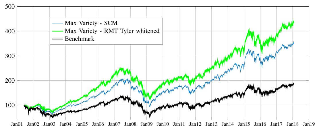
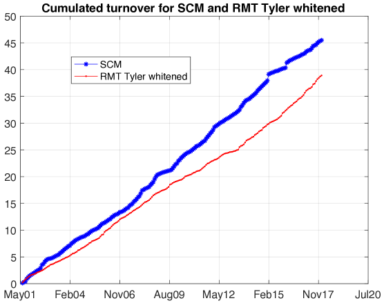
Figure 2: Left: portfolios wealth starting at $100$ at the first period. Right: cumulative sum of absolute weight changes (turnover) between the consecutive periods.

On the left of Figure 2, we report the evolution of portfolios wealths, starting at $100$ at the beginning of the first period. The Variety Max ”SCM” and ”RMT Tyler whitened” portfolios are respectively in blue and green and the price of the benchmark is the black line. The proposed RMT Tyler whitened technique clearly outperforms conventional ones. On the right of this figure, the cumulative turnover is shown for the both portfolios. We assume that the turnover (or the change in weights) between two consecutive periods $t$ and $t+1$ is measured by $\sum_{i=1}^{m}|w_{i,t+1}-w_{i,t}|$. Again, the proposed technique leads to lower the cumulated turnover which is important in finance. Limiting the turnover is often added as an additional non linear constraint to the optimization process (2). Figure 3 shows two different results. The two graphs on the left represent the evolution of the weights, on the overall period. Each colour represents an asset and the weights are stacked at each time (with the sum equals to one). The evolution of the weights for the Variety Max ”RMT Tyler whitened” portfolio is smoother than for the SCM. This is confirmed by a lower turnover too, so that the allocation process is more stable when using the proposed methodology. On the right of the same figure, we report the values of the selected eigenvalues (on the left axis) and its number as well (on the right axis). Most of the time, five eigenvalues are detected. This results show a different picture than the general one where only one source (the ”market”) is outside the Marčenko-Pastur bound. As noticed before, we get the same improvements as with other allocation process such as the Global Minimum Variance Portfolio.

TABLE I: Some performance numbers.

Variety Max	Ann.	Ann.	Ratio	Max
Portfolios	Return	Volatility	(Ret / Vol)	DD
RMT Tyler Whithened	9,71%	12,9%	0,75	50,41%
SCM	8,51%	13,80%	0,62	55,02%
Benchmark	4,92%	15,19%	0,32	58,36%

We finally report on table I some statistics on the overall portfolio performance: we compare, for the whole period, the annualised return, the annualised volatility, the ratio between the return and the volatility and the maximum drawdown of the portfolios and the benchmark. All the qualitative indicators related to the proposed technique show a significant improvement.

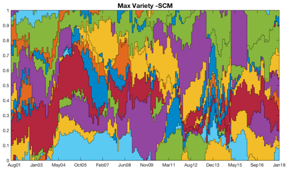
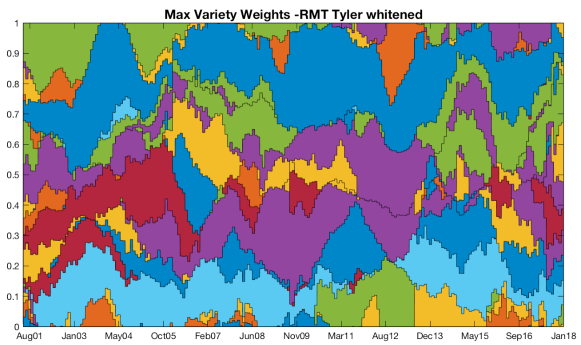
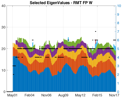
Figure 3: Left and middle: dynamic weights as a stacked area chart. Each colour represents an asset. The Variety Max ”RMT Tyler whitened” weights change smoother than the ones obtained with SCM, confirmed also by a smaller cumulative turnover. Right: values of the selected eigenvalues (left axis) and their number (right axis).

.

VI conclusion

In this paper we have shown that when processed correctly the Maximum Variety Portfolio allocation process leads to improved performance with respect to a classical approach. The improvement comes especially from the robust and denoised version of the covariance matrix estimate. Indeed, we have modelled the assets returns as a multi-factor model embedded in a correlated elliptical and symmetric noise, allowing to account for non-Gaussian and non correlated noise. Given this model setup, then we show how to separate the signal from the noise subspace using a ”toeplitzified” robust and consistent Tyler-M estimator and the Random Matrix theory applied on the whitened covariance matrix estimate. This paper has taken the Maximum Variety Portfolio process as an example but the same results apply on other allocation framework involving covariance matrix estimation (and/or model order selection), such as the Global Minimum Variance Portfolio. Moreover this can also be exploited to define the main directions of information and to construct pure factor driven models. These methods have also shown their importance in the radar and hyperspectral fields and are very promising techniques for many applications.

Acknowledgments

We would like to thank DGA and Fideas Capital for supporting this research and providing the data. We thank particularly Thibault Soler, and also Pierre Filippi and Alexis Merville for their constant interaction with the research team at Fideas Capital.

References

- [1] H. M. Markowitz, “Portfolio selection,” Journal of Finance, vol. 7, no. 1, pp. 77–91, 1952.
- [2] R. Clarke, H. D. Silva, and S. Thorley, “Minimum variance, maximum diversification, and risk parity: an analytic perspective,” Journal of Portfolio Management, June 2012.
- [3] S. Maillard, T. Roncalli, and J. Teiletche, “The properties of equally weighted risk contributions portfolios,” Journal of Portfolio Management, vol. 36, pp. 60–70, 2010.
- [4] Y. Choueifaty and Y. Coignard, “Toward maximum diversification,” Journal of Portfolio Management, vol. 35, no. 1, pp. 40–51, 2008.
- [5] Y. Choueifaty, T. Froidure, and J. Reynier, “Properties of the most diversified portfolio,” Journal of investment strategies, vol. 2, no. 2, pp. 49–70, 2013.
- [6] D. E. Tyler, “A distribution-free -estimator of multivariate scatter,” The annals of Statistics, vol. 15, no. 1, pp. 234–251, 1987.
- [7] R. A. Maronna, “Robust -estimators of multivariate location and scatter,” Annals of Statistics, vol. 4, no. 1, pp. 51–67, January 1976.
- [8] Y. Chen, A. Wiesel, and A. O. Hero, “Robust shrinkage estimation of high-dimensional covariance matrices,” IEEE Transactions on Signal Processing, vol. 59, no. 9, September 2011.
- [9] F. Pascal, Y. Chitour, and Y. Quek, “Generalized robust shrinkage estimator and its application to STAP detection problem,” IEEE Transactions on Signal Processing, vol. 62, no. 21, November 2014.
- [10] Y. Abramovich and N. K. Spencer, “Diagonally loaded normalised sample matrix inversion (LNSMI) for outlier-resistant adaptive filtering,” in IEEE Int. Conf. Acoust., Speech, Signal Process. (ICASSP), vol. 3, April 2007.
- [11] O. Ledoit and M. Wolf, “A well-conditioned estimator for large-dimensional covariance matrices,” Journal of Multivariate Analysis, vol. 88, pp. 365–411, 2004.
- [12] R. Couillet, F. Pascal, and J. W. Silverstein, “Robust estimates of covariance matrices in the large dimensional regime,” IEEE Transactions on Information Theory, vol. 60, no. 11, September 2014.
- [13] L. Yang, R. Couillet, and M. R. McKay, “A robust statistics approach to minimum variance portfolio optimization,” IEEE Transactions on Signal Processing, vol. 63, no. 24, pp. 6684–6697, Aug 2015.
- [14] W. F. Sharpe, “Capital asset prices: A theory of market equilibrium under conditions of risk,” Journal of Finance, vol. 19, no. 3, pp. 425–442, 1964.
- [15] L. Laloux, P. Cizeau, J.-P. Bouchaud, and M. Potters, “Noise dressing of financial correlation matrices,” Physycal Review Letters, vol. 83, no. 1468, 1999.
- [16] L. Laloux, P. Cizeau, M. Potters, and J.-P. Bouchaud, “Random Matrix Theory and financial correlations,” International Journal of Theoretical and Applied Finance, vol. 3, no. 03, pp. 391–397, 2000.
- [17] M. Potters, J. P. Bouchaud, and L. Laloux, “Financial applications of Random Matrix Theory: old laces and new pieces,” Acta Physica Polonica B, vol. 36, no. 9, 2005.
- [18] V. Plerou, P. Gopikrishnan, B. Rosenow, L. A. N. Amaral, and H. E. Stanley, “Collective behavior of stock price movements: A Random Matrix Theory approach,” Physica A, vol. 299, pp. 175–180, 2001.
- [19] J. Vinogradova, R. Couillet, and W. Hachem, “Statistical inference in large antenna arrays under unknown noise pattern,” IEEE Transactions on Signal Processing, vol. 61, no. 22, pp. 5633–5645, Nov 2013.
- [20] E. Terreaux, J. P. Ovarlez, and F. Pascal, “Robust model order selection in large dimensional Elliptically Symmetric noise,” arXiv preprint, https://arxiv.org/abs/1710.06735, 2017.
- [21] ——, “New model order selection in large dimension regime for Complex Elliptically Symmetric noise,” in 25th European Signal Processing Conference (EUSIPCO), Aug 2017, pp. 1090–1094.
- [22] ——, “A Toeplitz-Tyler estimation of the model order in large dimensional regime,” in IEEE International Conference on Acoustics, Speech and Signal Processing (ICASSP), Apr 2018.
- [23] D. Kelker, “Distribution theory of spherical distributions and a location-scale parameter generalization,” Sankhyā: The Indian Journal of Statistics, Series A, vol. 32, no. 4, pp. 419–430, 1970.
- [24] E. Ollila, D. E. Tyler, V. Koivunen, and H. V. Poor, “Complex Elliptically Symmetric distributions: Survey, new results and applications,” IEEE Transactions on Signal Processing, vol. 60, no. 11, pp. 5597–5625, Nov 2012.
- [25] J. M. Bioucas-Dias, A. Plaza, N. Dobigeon, M. Parente, Q. Du, P. Gader, and J. Chanussot, “Hyperspectral unmixing overview: Geometrical, statistical, and sparse regression-based approaches,” IEEE Journal of Selected Topics in Applied Earth Observations and Remote Sensing, vol. 5, no. 2, pp. 354–379, 2012.
- [26] D. Melas, R. Suryanarayanan, and S. Cavaglia, “Efficient replication of factor returns,” July 2009, MSCI Barra Research Paper No. 2009-23.
- [27] E. Jay, P. Duvaut, S. Darolles, and A. Chrétien, “Multi-factor models: examining the potential of signal processing techniques,” IEEE Signal Processing Magazine, vol. 28, no. 5, September 2011.
- [28] S. Darolles, P. Duvaut, and E. Jay, Multi-factor models and signal processing techniques: Application to quantitative finance. John Wiley & Sons, 2013.
- [29] S. Darolles, C. Gouriéroux, and E. Jay, “Robust portfolio allocation with risk contribution restrictions,” in Forum GI - Paris, March 2013.
- [30] F. Pascal, Y. Chitour, J. P. Ovarlez, P. Forster, and P. Larzabal, “Covariance structure maximum-likelihood estimates in compound Gaussian noise: Existence and algorithm analysis,” IEEE Transactions on Signal Processing, vol. 56, no. 1, pp. 34–48, Jan 2008.
- [31] F. Pascal, P. Forster, J. P. Ovarlez, and P. Larzabal, “Performance analysis of covariance matrix estimates in impulsive noise,” IEEE Transactions on Signal Processing, vol. 56, no. 6, pp. 2206–2217, June 2008.
- [32] M. Mahot, F. Pascal, P. Forster, and J. P. Ovarlez, “Asymptotic properties of robust complex covariance matrix estimates,” IEEE Transactions on Signal Processing, vol. 61, no. 13, pp. 3348–3356, July 2013.
- [33] R. Couillet and M. Debbah, Random matrix methods for wireless communications. Cambridge University Press, 2011.
- [34] S. Kritchman and B. Nadler, “Non-parametric detection of the number of signals: Hypothesis testing and random matrix theory,” IEEE Transactions on Signal Processing, vol. 57, no. 10, pp. 3930–3941, Oct 2009.
- [35] R. Couillet, M. S. Greco, J. P. Ovarlez, and F. Pascal, “RMT for whitening space correlation and applications to radar detection,” in IEEE CAMSAP, Dec 2015, pp. 149–152.
- [36] W. Hachem, P. Loubaton, X. Mestre, J. Najim, and P. Vallet, “A subspace estimator for fixed rank perturbations of large random matrices,” Journal of Multivariate Analysis, vol. 114, pp. 427–447, 2013.
- [37] R. Couillet, “Robust spiked random matrices and a robust G-MUSIC estimator,” Journal of Mult. Analysis, vol. 140, pp. 139–161, 2015.
- [38] V. A. Marchenko and L. A. Pastur, “Distribution of eigenvalues for some sets of random matrices,” Matematicheskii Sbornik, 1967.
- [39] Stoxx, “Stoxx europe 600 index,” https://www.stoxx.com/index-details?symbol=SXXP.