Robust Wald-type tests in GLM with random design based on minimum density power divergence estimators
Abstract
We consider the problem of robust inference under the generalized linear model (GLM) with stochastic covariates. We derive the properties of the minimum density power divergence estimator of the parameters in GLM with random design and use this estimator to propose robust Wald-type tests for testing any general composite null hypothesis about the GLM. The asymptotic and robustness properties of the proposed tests are also examined for the GLM with random design. Application of the proposed robust inference procedures to the popular Poisson regression model for analyzing count data is discussed in detail both theoretically and numerically through simulation studies and real data examples.
Keywords and phrases: GLM; Minimum density power divergence estimator; Wald-type tests; Robustness.
1 Introduction
Parametric statistical modelling is an important tool in statistical analysis of real data. Whenever the parametric assumption is satisfied, the parametric method will be much more efficient than the corresponding non-parametric methods. However, classical parametric methods, including those based on the maximum likelihood principle, can be very significantly influenced by the presence of outlying observations in the data, even in a very small proportion. The data analyst would, therefore, like to construct and use such procedures which exhibit a high degree of robustness (in the sense of outlier stability) with little loss in asymptotic efficiency. In the current age of big data, the outlier problem is as relevant as ever. In this paper we will deal with the robustness issue in case of generalized linear models where the covariates are stochastic (rather than fixed).
Regression analysis is a basic statistical data analysis technique across different disciplines of applied sciences, which helps us to model a response variable in terms of several associated covariates. One major application of regression is also in predicting future observations from the values of the model covariates as well as in investigating if a covariate has a statistically significant role in explaining the variability in the response. The standard linear regression model is the most common one applicable to a continuous response having a linear relationship with each covariate. We consider a much wider class of regression models, namely generalized linear models (GLMs), first introduced by Nelder and Wedderburn (1972) and later expanded by McCullagh and Nelder (1989); they represent a method of extending standard linear regression to incorporate a variety of responses including distributions of counts, binary or positive values as well as several types of possible relationship between the response and covariates (under suitable restrictions). Here, the observations are assumed to be independent and identically distributed (IID) realizations of the random variables in such a way that the conditional distribution of given belongs to the general exponential family of distributions having density function, with respect to a convenient -finite measure, given by
| (1) |
where the canonical parameter is an unknown measure of location depending on the predictor and is a known or unknown nuisance scale or dispersion parameter typically required to produce standard errors following Gaussian, gamma or inverse Gaussian distributions. The functions , and are known. In particular, is set to for binomial, Poisson, and negative binomial distributions (known ), and it does not enter into the calculations for standard errors. The mean of the conditional distribution of given , namely , is dependent only on and is assumed, according to GLMs, to be modeled linearly with respect to through a known link function, , i.e., where is a monotone and differentiable function and is an unknown parameter. In this setting, since , we shall also denote the density in (1) by . The statistical problem is then to first estimate the regression coefficients and the variance parameter (if unknown) through appropriate estimation methods like maximum likelihood estimation and use these estimates for subsequent hypotheses testing and prediction for the underlying research applications.
To clarify the objective of the present paper, we note that the matrix is referred to as the design matrix in the context of regression. As per the above formulations, all rows of this design matrix are IID copies of the -dimensional (covariate) random variable . Such situations are referred to as the random design models which we focus on the present paper. Another alternative option, mostly used for planned design of experiments, is the fixed design models where each row of the design matrix is assumed to be non-stochastic and pre-fixed. One can verify that for most common applications, if we assume fixed design set-up while the values of each row actually came from some underlying distributions, the estimators of would be identical to the random design case but their asymptotic properties (including the variance and hence the standard errors) may be quite different depending on the stochastic structure of the true random design matrix which, in turn, affects the hypotheses testing results and any predictive confidence intervals. This can be illustrated through a simple example of maximum likelihood estimator (MLE) of under the simple linear regression model, a special case of GLM with and the identity link (). In this particular example, the MLE is with for both of fixed and random designs, but the asymptotic variance are given, respectively, by for fixed design and for the random design. Now, suppose the random design is true having , with and ; then ideally the asymptotic variance of MLE of should be , a constant independent of the observed data. However, if one wrongly assume that the design matrix is fixed based on the observed data, the corresponding asymptotic variance matrix will turn out to be , which can clearly be substantially different from the true based on the observed data for finite sample sizes (e.g., may be heavy tailed), and consequently all the inferential results (testing and confidence intervals) could be adversely affected. This motivated the study of GLMs having random design matrices separately from the fixed design cases.
However, the usual inference procedures based on the maximum likelihood and the maximum quasi-likelihood estimators are extremely non-robust against the data contaminations or model misspecification under both the fixed or random design set up; these have been studied extensively in the literature for different GLMs and their non-robustness have been demonstrated by several authors (Hampel et al. 1986; Stefanski et al., 1986; Künsch et al., 1989; Morgenthaler, 1992, and many others). Modern complex datasets are prone to having outlying observations either due to some confounded effects or error in any stage of data processing which, in turn, yields incorrect statistical results and research insights if a non-robust method is used to analyze them. Consequently, robust procedures for GLMs have been considered to robustify the MLE. Stefanski et al. (1986) studied optimally bounded score functions for the GLM. They generalized the results obtained by Krasker and Welsch (1982) for classical linear models. The robust estimator of Stefanski et al. (1986) is, however, difficult to compute. Künsch et al. (1989) introduced another estimator, called the conditionally unbiased bounded-influence estimator. The development of robust models for the GLM continued with the work of Morgenthaler (1992). More recently, Cantoni and Ronchetti (2001) proposed a robust approach based on robust quasi-deviance functions for estimation and variable selection. Another class of estimators are the M-estimators proposed by Bianco and Yohai (1996) and further studied by Croux and Haesbroeck (2003) for logistic regression, a special case of GLMs. Bianco et al. (2013) proposed general M-estimators for GLM for data sets with missing values in the responses. Valdora and Yohai (2014) proposed a family of robust estimators for GLM based on M-estimators after applying a variance stabilizing transformation to the response. More recent works on robust inference in GLMs also include Aeberhard et al. (2014) and Marazzi et al. (2019). Along this line of research, Ghosh and Basu (2016) presented a robust estimator assuming a fixed design, based on the density power divergence approach. In this paper, we will first extend it to the random design GLMs and subsequently discuss its properties in developing robust hypotheses testing procedures. Throughout this paper, our focus will be on robustness against data contamination (e.g., outliers) among the sample observations and discuss the properties of the proposed estimators and tests in respect of safeguarding against such data contamination.
To define our estimator for the random design GLMs as discussed above, we note that the observations indeed form a random sample from and the density function of is denoted as . For the cases of non-random design with fixed , Ghosh and Basu (2016) considered a particular class of -estimators depending on a tuning parameter , which solved the estimating equation
where
| (2) |
with and if is unknown, and , otherwise. In Ghosh and Basu (2016) it was established that
for unknown , where
Therefore, defining
| (3) |
we get
and the estimating equations are given by
| (4) | ||||
| (5) |
Notice that for known , the unique estimating equation is (4). It is clear that
when the conditional distribution of given the covariates belongs to the assumed GLM family and hence the estimators considered in Ghosh and Basu (2016) are conditionally Fisher-consistent at the model for random design as well. In addition, since
| (6) |
these estimators are also unconditionally Fisher consistent under random design GLMs as well. Let us denote as the estimator of , obtained by solving equations (4) and (5), which we refer to as the minimum density power divergence estimator (MDPDE) of . Under suitable differentiability properties of the functions , , and , the equations (4) and (5) are indeed the estimating equations for obtaining the MDPDEs of the parameter ; see Basu et al. (1998), Ghosh and Basu (2013) and Ghosh and Basu (2016) for a general description of the density power divergence as well as the formulation of the divergence in the generalized linear models scenario. Ghosh and Basu (2016) derived the asymptotic distribution of assuming that , , are non-random (fixed design).
The primary purpose of this paper is to present the asymptotic distribution as well as the robustness properties of the minimum density power divergence estimator when , , are generated by a random design. These are seen to be quite different from those developed under the fixed-design set-up in Ghosh and Basu (2016) and may be hampered in the same way as illustrated earlier for the MLEs if the design matrix is wrongly assumed to be fixed. Subsequently, based on the estimator , a family of robust Wald-type tests is introduced. The properties of the test statistics depend directly on the newly derived properties of the estimator; we study the asymptotic and robustness properties along with appropriate numerical illustrations.
The structure of the paper is as follows. In Section 2 we present the asymptotic distribution of the MDPDE of for the random design case. Section 3 introduces Wald-type tests for testing general linear hypothesis on parameters under study and establishes their asymptotic distribution. The robustness properties of the Wald-type tests are studied in Section 4. The Poisson regression model under the random design is studied in Section 5, and finally, Section 6 presents a detailed simulation study illustrating the benefits of our proposal.
2 Properties of the MDPDEs under Random Design
Together with the notation of Section 1, let us assume that represents the vector of (random) explanatory variables and the marginal distribution of is denoted by . In the following we first consider the asymptotic properties of the MDPDE and thereafter, study the corresponding robustness properties.
2.1 Asymptotic Properties
In order to derive the asymptotic distribution of , we are going to follow the same scheme as given in Theorem 10.7 of Maronna et al. (2006) for M-estimators. Through this, the asymptotic distribution of is given by
where with
Here, is the sample space of . After some algebra, the expressions turn out to be
and
where , , is given by (3) and
Notice that for the case where is known, we get and .
2.2 Robustness Properties: Influence Function
Let us now study the robustness of the MDPDEs of through the classical influence function of Hampel et al. (1986). Let us rewrite the MDPDE in terms of a statistical functional at the true joint distribution of as the solution of (6), whenever it exists. Consider the contaminated distribution , where is the contamination proportion and is the degenerate distribution at the contamination point . Then, the influence function of is defined as
| (7) |
which measures the bias in the estimator due to an infinitesimal contamination in the data generating distribution. Thus, a bounded influence function indicates local stability in the estimators in terms of bounding the bias under contamination, which is referred to as (local) B-robustness. Although there are several other important robustness measures as briefly pointed out later in Section 8, throughout the present paper we will indicate such local B-robustness whenever we talk about robustness of our MDPDE and the corresponding tests in terms of having a bounded influence function.
Note that, the MDPDE functional is clearly an M-estimator functional and we can get its influence function directly from existing M-estimator theory. In particular, the influence function of the MDPDE functional at the model distribution is given by
| (10) |
where is as defined in Section 2.1 and is the point of contamination.
Further, suppose and refer to the MDPDE functionals corresponding to the parameters and , respectively, so that . Note that the influence functions of the two estimators and are not independent in general linear models. However, whenever the matrix is diagonal (as in the normal linear model) or is known (as in the logistic and Poisson regression models), the influence function of the MDPDE of can be written simply as
| (11) |
From the above form it is easily observed that this influence function is bounded in the contamination point for all and unbounded at for most standard GLMs. For example, under the normal linear regression model, the influence function of the MDPDE of depends on the contamination point through the quantity and hence it is bounded for all implying the robustness of the corresponding MDPDEs. In this paper we will present the general theory of the random design model, and illustrate the methodology in detail for the Poisson regression problem.
3 Wald-type Test Statistics for General Composite Hypothesis
The asymptotic distribution of , given in Section 2.1, will be useful in order to define a family of Wald-type test statistics for testing the null hypothesis
| (12) |
with . Thus the null hypothesis imposes restrictions on the parameter . We shall assume that is a continuous full (column) rank matrix with rows and columns.
If is known or we are only interested in testing some hypothesis on , say, , we shall consider and then if is unknown, and if is known. The most commonly used hypothesis under this set-up is the general linear hypothesis on given by for some matrix and -vector . Here we have and or for unknown or known respectively. On the other hand, if we are interested in testing , we shall consider In this case .
Definition 1
Let be the MDPDE for . The family of Wald-type test statistics for testing the null hypothesis given in (12) is given by
| (13) |
Theorem 2
Proof. We know that and because . Therefore
Then the asymptotic distribution of is a chi-square distribution with degrees of freedom.
Based on the previous theorem the null hypothesis given in (12) will be rejected at if we have
| (14) |
Now we consider such that , i.e., does not belong to the null hypothesis. We denote
and, in the following, we provide an approximation to the power function for the Wald-type tests given in (14).
Theorem 3
Let be the true value of the parameter such that and . The power function of the tests given in (14), in , is given by
| (15) |
where almost surely converges to the standard normal distribution and is given by
Proof. We have
Now we are going to get the asymptotic distribution of the random variable . Since , it is clear that and have the same asymptotic distribution. The first order Taylor expansion of around , evaluated at , gives
Therefore, it holds
and the result follows.
Remark 4
Based on the previous theorem, we can obtain the sample size necessary to get a specific power . From (15), we must solve the equation
and we get that with
where
Corollary 5
Under the assumptions of Theorem 3, we have as Thus, our proposed Wald-type tests are consistent at any fixed alternative.
We may also find an approximation of the power of the Wald-type tests given in (13) at an alternative close to the null hypothesis. Let be a given alternative and let be the element in boundary of closest to in the Euclidean distance sense. One possibility to introduce contiguous alternative hypotheses in this set up is to consider a fixed vector and to permit to move towards with increasing as
| (16) |
A second approach could be to relax the condition defining Let and consider the sequence of parameters moving towards according to
| (17) |
Note that a Taylor series expansion of around yields
| (18) |
By substituting in (18) and taking into account that , we get
so that the equivalence of the two approaches in the limit is obtained for .
In the following we shall denote by the non-central chi-square random variable with degrees of freedom and non-centrality parameter .
Theorem 6
We have the following results under both versions of the contiguous alternative hypothesis:
Proof. A Taylor series expansion of around yields
From (18), we have
As and
we have
We can observe by the relationship , if that
We apply the following result from Anderson (2003) concerning quadratic forms. “If , is a symmetric projection of rank and , then is a chi-square distribution with degrees of freedom and noncentrality parameter ”. In our case, the quadratic form is
with
and
where is the identity matrix. Hence, the application of the result is immediate and the noncentrality parameter is
4 Robustness of the Proposed Wald-type Test Statistics
4.1 Influence Function of the Wald-type Test Statistics
In order to study the robustness of the proposed Wald-type tests of Section 3, we will start with the influence function of the Wald-type test statistics in (13) for testing the general composite hypothesis (12). Consider the MDPDE functional at the true joint distribution of as defined in Section 2.2 and define the statistical functional corresponding to the Wald-type test statistics at as (ignoring the multiplier )
| (19) |
Again, considering the contaminated distribution, , the influence function of the Wald-type test functional is given by
Suppose be the true parameter value under null hypothesis given in (12) that satisfies and the corresponding null joint distribution be . Note that, under , by Fisher consistency of the MDPDE and hence . Hence, the first order influence function cannot portray the robustness of the proposed Wald-type tests (like other Wald-type tests in Rousseeuw and Ronchetti, 1979; Toma and Broniatowski, 2011; Ghosh et al., 2016, etc.) and we need to derive its second order influence function.
By another differentiation, we get the second order influence function of at as given by
Note that the influence function of the test statistic is directly related to the influence function of the corresponding estimator. In particular, at the null distribution , we get the nonzero second order influence function indicating the robustness properties of the proposed Wald-type test statistics. These are summarized in the following theorem.
Theorem 7
The influence functions of the proposed Wald-type test statistics at the null distribution is given by
Clearly, the second order influence function is bounded whenever the function is bounded, i.e., for all , implying the robustness of the proposed Wald-type tests with . However, at , and hence the second order influence function is unbounded implying the non-robust nature of the classical MLE based Wald-test.
4.2 Level and Power Robustness
Let us now study the stability of the level and the power of the proposed Wald-type test statistics under data contamination. For this, we will derive the level and power influence functions respectively under the null hypothesis and the contiguous alternative hypotheses in (16). Considering contamination over these hypothesis as in Hampel et al. (1986) and Ghosh et al. (2016), we define the LIF and PIF respectively through the asymptotic distribution under
where denote the joint model distribution of with parameter , given by . For the proposed Wald-type test statistics , its LIF and PIF are defined by
and
Theorem 8
Under the assumptions of Theorem 5, we have the following:
-
1.
Under , the proposed Wald-type test statistics asymptotically follows a non-central chi-square distribution with degrees of freedom and non-centrality parameter
(20) where
-
2.
The asymptotic power function under can be approximated as
(21) where
Proof. Let us denote . Then, the asymptotic distribution of the MDPDE under yields
| (22) |
Now, using a suitable Taylor series approximation and the above asymptotic distribution, we get
Again, another Taylor series approximation yields
| (23) |
and hence
| (24) |
using . Therefore, combining all the above results, we get
where
But, by (22),
which implies that a non-central random variable with degrees of freedom and non-centrality parameter as defined in (20).
The second part of the theorem follows by the infinite series expansion of a the above non-central distribution in terms of the central chi-square variables as
Note that, substituting in Theorem 8, we get an alternative expression for the asymptotic power function of our proposed Wald-type test statistics under the contiguous alternatives as
Further, substituting in Theorem 8, we can derive the asymptotic distribution of the Wald-type test statistics under which is non-central chi-square with degrees of freedom and non-centrality parameter
Therefore, the asymptotic level under contiguous contamination turns out to be
Note that, as , , the nominal level of the test.
Using the above expressions for asymptotic power and level under contiguous contamination, one can easily derive the PIF and LIF of the proposed Wald-type test statistics as described in the following theorem.
Theorem 9
Assume the conditions of Theorem 8 hold. Then, the power and level influence functions of our proposed Wald-type tests based on is given by
| (25) |
with and
and
Also, the level influence function of any higher order is also identically zero.
Proof. The proof follows by differentiating the expression of from Theorem 8 with respect to using the chain rule and is similar to that of Theorem 8 of Ghosh et al. (2016).
Note that the above theorem implies the stability of the asymptotic level of our proposed Wald-type tests with respect to the infinitesimal contamination for any . On the other hand the power influence function is bounded implying the stability of the asymptotic contiguous power only when the influence function of the MDPDE is bounded, i.e., for . The PIF of the classical Wald-type test based on MLE (at ) is unbounded indicating its well-known non-robust nature.
5 Application: Poisson Regression Model under Random Design
Poisson regression is a very popular member of the class of GLMs where the underlying distribution, given by the density , is Poisson with mean , so that
Hence, in terms of the general model density given in Equation (1), we have and , , and the link function is the natural logarithm function. Also, note that . Additionally, we assume that the covariates are random having distribution function , which is generally normal for continuous covariates. This regression model is widely used in practice for modeling count data like total number of occurrences of a particular disease in medical sciences, number of failures in reliability or survival analysis, etc.
Note that, as known for the case of Poisson regression the parameter of interest is . The MDPDE of can then be obtained by solving only one (unbiased) estimating equation (4) which has the simplified form for Poisson regression as
| (26) |
where For the particular case of , we have and hence this estimating equation further simplifies to
| (27) |
which is nothing but the likelihood score equation of the maximum likelihood estimator (MLE) of .
Now, the asymptotic distribution of the MDPDE of can be derived directly from the results of Section 2.1. In particular, under the model distribution with true parameter value , we have
where we now have and with At , one can show that and hence , which is exactly the Fisher information matrix under the present set-up generating the asymptotic distribution of the MLE . Based on these asymptotic distributions, one can compute the asymptotic relative efficiencies of our MDPDEs over which are presented in Table 1 for the case of a scalar () normally distributed covariate . Clearly, as expected from the literature of the MDPDE in any other model, the ARE decreases slightly as increases but this loss in efficiency is not substantial at small positive . And, with this small price in asymptotic efficiency, we gain high robustness properties of our MDPDEs with .
| 0 | 0.05 | 0.1 | 0.25 | 0.4 | 0.5 | 0.7 | 1 | ||
|---|---|---|---|---|---|---|---|---|---|
| 0 | 1 | 1.000 | 0.995 | 0.985 | 0.927 | 0.849 | 0.793 | 0.671 | 0.489 |
| 0 | 0.5 | 1.000 | 0.996 | 0.985 | 0.931 | 0.861 | 0.811 | 0.713 | 0.576 |
| 1 | 1 | 1.000 | 0.995 | 0.986 | 0.932 | 0.859 | 0.807 | 0.701 | 0.550 |
| 1 | 0.5 | 1.000 | 0.997 | 0.988 | 0.940 | 0.880 | 0.839 | 0.757 | 0.646 |
| 5 | 1 | 1.000 | 0.996 | 0.986 | 0.927 | 0.848 | 0.791 | 0.676 | 0.516 |
| 5 | 0.5 | 1.000 | 0.996 | 0.987 | 0.937 | 0.872 | 0.826 | 0.736 | 0.615 |
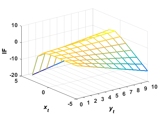
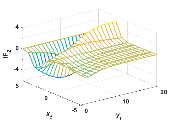
To see such robustness advantages of our MDPDEs , we consider the influence function of the MDPDE functional of from Section 2.2. This influence function can be simplified for the present case of Poisson regression model at the model distribution with parameter value as
Note that the above influence function is bounded at and unbounded at . This implies the robustness of the MDPDEs with and the non-robust nature of the MLE at . In particular, the influence function of the MLE under the Poisson regression model is a straight line (unbounded in both outliers in response, , and leverage points in covariate space, ) and is given by
Figure 1 presents these influence functions for different , when is a scalar () continuous variable having a normal distribution. Note that the influence function of the classical Wald test at is unbounded for for any fixed (outlier in response) as well as for with small or with larger (leverage points). On the contrary, influence functions of the MDPDEs with are bounded in both the cases indicating their robustness against outliers in both and -spaces. Also, the nature of the influence function (and hence robustness of the corresponding estimators) remains invariant with respect any change in the covariate mean (only the magnitude of the influence function changes). Further, the supremum of the IF in absolute value decreases as increases, indicating the increasing robustness of the MDPDEs with increasing .

Now, consider the problem of testing the general linear hypothesis of under the Poisson regression model, i.e., consider the hypothesis
| (28) |
where is a full rank matrix of order , with (), and is an -dimensional vector, both of known values. We assume that . This clearly belongs to the general class of hypothesis considered in (12) with and (since is known here). Then the proposed MDPDE based Wald-type test statistics for testing (28) is given by
| (29) |
By Theorem 2, under , the above Wald-type test statistics asymptotically follow a distribution. The tests are also consistent at any fixed alternative from Corollary 5. We will now derive their asymptotic power under contiguous alternatives , where is the true null parameter value satisfying . From Theorem 6, we get the asymptotic distribution of our Wald-type test statistic to be a non-central chi-square distribution with degrees of freedom and non-centrality parameter . Hence the asymptotic contiguous power can be obtained from the distribution function of this non-central chi-square distribution, which is presented in Table 2 for the case with a normally distributed covariate . One can clearly observe that the asymptotic contiguous power for any fixed decreases slightly with increasing , but the loss in power in not quite significant. Notice the similarity with the nature of ARE of the corresponding MDPDE from Table 1, because the asymptotic contiguous power is directly related to the asymptotic variance (and hence to the asymptotic efficiency) of the estimator used.
| 0 | 0.05 | 0.1 | 0.25 | 0.4 | 0.5 | 0.7 | 1 | |||
|---|---|---|---|---|---|---|---|---|---|---|
| 1 | 0 | 1 | 0.445 | 0.443 | 0.440 | 0.418 | 0.389 | 0.368 | 0.320 | 0.247 |
| 1 | 0 | 0.5 | 0.236 | 0.235 | 0.233 | 0.222 | 0.209 | 0.200 | 0.181 | 0.156 |
| 1 | 1 | 1 | 0.998 | 0.998 | 0.997 | 0.996 | 0.993 | 0.990 | 0.979 | 0.943 |
| 1 | 1 | 0.5 | 0.669 | 0.667 | 0.663 | 0.642 | 0.613 | 0.593 | 0.550 | 0.486 |
| 1 | 5 | 1 | 1.000 | 1.000 | 1.000 | 1.000 | 1.000 | 1.000 | 1.000 | 1.000 |
| 1 | 5 | 0.5 | 1.000 | 1.000 | 1.000 | 1.000 | 1.000 | 1.000 | 1.000 | 1.000 |
| 2 | 0 | 1 | 0.954 | 0.953 | 0.951 | 0.939 | 0.919 | 0.900 | 0.847 | 0.721 |
| 2 | 0 | 0.5 | 0.696 | 0.695 | 0.690 | 0.665 | 0.632 | 0.606 | 0.551 | 0.467 |
| 2 | 1 | 1 | 1.000 | 1.000 | 1.000 | 1.000 | 1.000 | 1.000 | 1.000 | 1.000 |
| 2 | 1 | 0.5 | 0.998 | 0.998 | 0.997 | 0.996 | 0.994 | 0.992 | 0.986 | 0.971 |
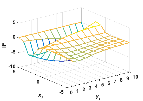
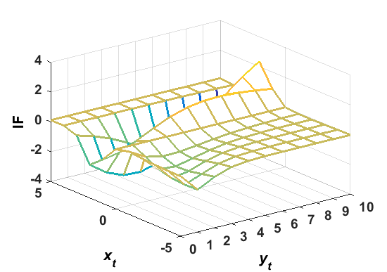
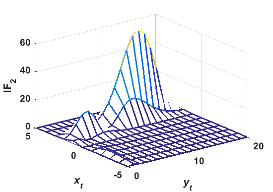
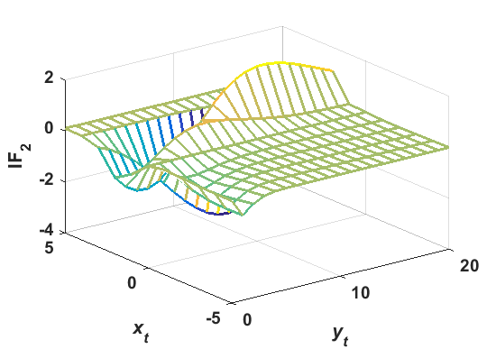
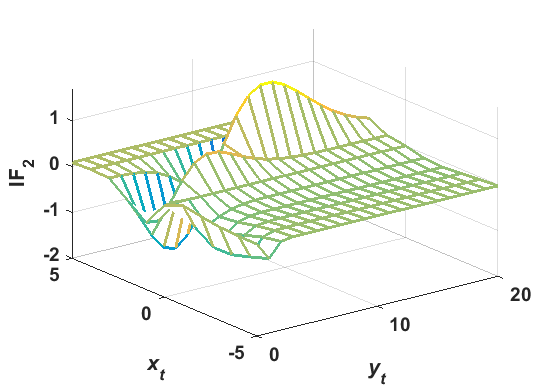
As in the case of the MDPDE, we indeed gain high robustness of the proposed Wald-type test statistics with at a small cost in asymptotic contiguous power. To see this, we consider the influence function analysis for the Poisson regression model following the general theory developed in Section 4. In particular, the first order influence function of the Wald-type test statistics is always zero and corresponding second order influence function for testing (28) under the Poisson regression model at the null distribution with true parameter value simplifies to
with Similarly, while considering the level and power robustness of the proposed Wald-type test statistics for testing (28) under Poisson regression model, the LIF is always zero from Theorem 9 and the PIF at the null distribution simplifies to
| (30) |
where now we have and is as defined in Theorem 9. Note that, both the second order influence function of the Wald-type test statistics and its power influence function are bounded for implying robustness of our proposal. On the other hand, both are unbounded at demonstrating the well-known non-robust nature of the classical Wald test. Figures 2 and 3, respectively, present these influence functions for the Poisson regression case with and a normally distributed covariate. Note that these influence functions are, respectively, a quadratic and a linear function of the corresponding influence function of the MDPDE (illustrated in Figure 1) used in constructing the Wald-type test statistics and demonstrate (appropriately transformed) bounded behavior. In particular, their redescending nature with respect to increasing is clearly seen from the figures which implies that the robustness of our proposed Wald-type test statistics increases with increasing .


6 Simulation Study
In this section, we will present some numerical illustrations for the finite sample performance of our proposed Wald-type tests under the Poisson regression model of the previous section through appropriate simulation results. We start with empirical demonstration of their robustness properties. We consider three explanatory variables in this study, so , where is a vector with all elements equal to one. The other three components of are independently generated from the standard normal distribution. The response variable is simulated from the Poisson distribution with mean parameter . The true value of the parameter is taken as . We consider the null hypothesis as . Let us define and
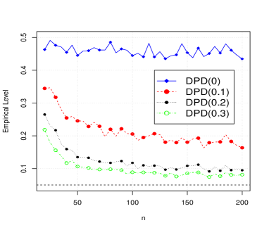
Then the null hypothesis can be written as . According to the set up of the simulation the null hypothesis is true. So, at first, our interest is to check whether or not the observed levels of different Wald-type tests match with the nominal level at . The total number of replications is taken as 2000 in this study. Here the observed level is measured as the proportion of test statistics exceeding the corresponding chi-square critical value in 2000 replications. The results are given in Figure 4(a) where the sample size varies from 20 to 200. We have used several Wald-type test statistics, corresponding to different MDPDEs. The values of the DPD tuning parameter are taken to be and , and the Wald-type test corresponding to is denoted by . As it is previously mentioned, is the classical Wald test for the Poisson regression model which uses the MLE. The horizontal line in the figure represents the nominal level of 0.05. It is noticed that all tests produce almost identical results – they are slightly liberal for small sample sizes and lead to somewhat inflated observed levels. However, this discrepancy decreases rapidly as the sample size increases.
In the next simulation study we evaluate the stability of the level of the tests under contamination. So, we repeated the tests for the same null hypothesis by adding 5% outliers in the data. For the outlying observations the values of the response variable were altered to . Figure 4(b) shows that the level of the classical Wald test completely breaks down, whereas Wald-type tests with and present stable levels. The performance of the Wald-type test with , though much more stable than the classical Wald test, is relatively poor.
To investigate the power of the Wald-type tests we took the same null hypothesis, but changed the true data generating parameter to , where and is a unit vector of length 4. The rest of the set up as well as values of and remained unchanged from the first experiment. The empirical power functions are calculated in the same manner as the levels of the tests and plotted in Figure 4(c). Here the classical Wald test is the most powerful under pure data. However, the performances of other Wald-type tests are also practically as good as the classical Wald test. Therefore, from Figures 4(a) and (c) we notice that there is hardly any difference among these tests in pure data in terms of the level and power.
Finally, we calculated the power functions of the above hypothesis under contaminated data. The true data generating parameter is taken as , where and 5% of the data are contaminated with . The observed powers of the Wald-type tests are given in Figure 4(d). All Wald-type test statistics show stable powers under contamination, and those powers are almost unchanged as observed in Figure 4(c). On the other hand, the classical Wald test exhibits a drastic loss in power. Notice that the observed level of the classical Wald test is already very high (around 0.45) at contaminated data, so it is expected to produce a large power just because of the inflated level. But due to their outlier stability, the power of the classical Wald test does not increase with the sample size at the same rate as the other robust tests. In fact, it shows a relatively significant drop over most of the range considered in our study. On the whole, the proposed Wald-type test statistics corresponding to moderately large appear to be quite competitive to the classical Wald test for pure data, but they are far better in terms of robustness properties under contaminated data.
| (a) | (b) |
 |
 |
| (c) | (d) |
 |
 |
| Level or | |||||
|---|---|---|---|---|---|
| Power | 0 | 0.1 | 0.2 | 0.3 | |
| Level | 0 | 0.056 | 0.049 | 0.044 | 0.043 |
| Power | 0 | 0.509 | 0.501 | 0.488 | 0.468 |
| Level | 0.05 | 0.989 | 0.077 | 0.064 | 0.070 |
| Power | 0.05 | 0.994 | 0.538 | 0.522 | 0.496 |
| 0 | 0.1 | 0.2 | 0.3 | |
|---|---|---|---|---|
| 100 | 0.084 | 0.063 | 0.064 | 0.071 |
| 200 | 0.165 | 0.120 | 0.127 | 0.136 |
| 500 | 0.380 | 0.353 | 0.341 | 0.323 |
| 1000 | 0.704 | 0.808 | 0.786 | 0.752 |
| 1500 | 0.906 | 0.967 | 0.959 | 0.959 |
| 2000 | 0.979 | 0.994 | 0.991 | 0.988 |
| 3000 | 1.000 | 1.000 | 1.000 | 1.000 |
In the next set of simulation studies, we consider a more general set up to explore the performance of the proposed Wald-type tests. Here we have taken ; the explanatory variables are generated independently from the standard normal distribution. To make the hypothesis general, we have arbitrarily chosen elements of vector , and dimensional matrix . Each element of and is generated from an independent and identically distributed uniform distribution from to 1. After that and are kept unchanged throughout the simulation. Suppose . In the first simulation, is generated from the Poisson distribution with mean parameter ; we are interested in verifying the levels of the Wald-type tests for testing the null hypothesis . We have taken a sample of size and replicate it a 1000 times. The first row of Table 3 shows that the empirical levels of all four tests are closely bunched around the nominal level of . Next, we explore the powers of these tests when the true value of the parameter is in slight deviation from . We generated from , where with . The results in the second row of Table 3 shows that the classical Wald test is the most powerful; however, other Wald-type tests also produce very competitive powers. In Table 4, we expand the exploration of the study of power for pure data (as in the second row of Table 3) over different sample sizes; the true parameter is taken very close to the null hypothesis where with . The result shows that the powers of all tests converge to one as sample size increases indicating the consistency of the proposed tests.
To check the robustness properties of these tests, we contaminated proportion outliers in the variable. Those outlying values are 25 standard deviations away from their respective means. The third row of Table 3 presents the empirical levels of the tests where there are 5% outliers and for the rest of the data set . The classical Wald test shows an extreme inflation of level in this case, whereas other Wald-type tests show a stable level. In the same set up, we checked the powers of the tests under contamination where 95% data are generated from . The powers of the robust Wald-type tests are very similar to the corresponding uncontaminated case. So, it shows that 5% contamination does not significantly affect the powers of these tests. Although, the observed power of the classical Wald test is very high, it is merely because of its inflated level. In fact, we could check that the actual level-corrected power is very poor in this situation.
While we have primarily used the influence function for the description of the robustness of our proposed tests, there are several other possible measures of robustness of statistical procedures. The breakdown point, which quantifies the degree of contamination that the procedure can withstand before it becomes completely uninformative, is one of them. Here we empirically explore the breakdown properties of our tests. In Table 5, the level robustness of the Wald type tests are demonstrated. The contamination scheme is as in the third row of Table 3, but the contamination proportion is slowly allowed to increase to 0.5. Clearly the observed level for the ordinary Wald test is pushed to the maximum possible value at fairly small levels of contamination, but for moderately large values of the observed levels remain substantially smaller than 1 even at .
| 0 | 0.1 | 0.2 | 0.3 | |
|---|---|---|---|---|
| 0 | 0.056 | 0.049 | 0.044 | 0.043 |
| 0.05 | 0.989 | 0.077 | 0.064 | 0.070 |
| 0.10 | 1.00 | 0.132 | 0.095 | 0.118 |
| 0.15 | 1.00 | 0.222 | 0.163 | 0.180 |
| 0.20 | 1.00 | 0.320 | 0.201 | 0.201 |
| 0.25 | 1.00 | 0.445 | 0.288 | 0.287 |
| 0.30 | 1.00 | 0.603 | 0.365 | 0.373 |
| 0.35 | 1.00 | 0.731 | 0.461 | 0.475 |
| 0.40 | 1.00 | 0.863 | 0.548 | 0.566 |
| 0.45 | 1.00 | 0.928 | 0.627 | 0.647 |
| 0.50 | 1.00 | 0.974 | 0.748 | 0.757 |
Finally, we did a study on the effect of leverage points on the Wald-type tests. In the previous simulation studies, the explanatory variables are generated independently from the standard normal distribution. Now, proportion of explanatory variables in the samples (of size ) are generated independently from . The remaining set up of the simulation is same as the set up in the first row of Table 3. Table 6 shows the levels of the Wald-type tests for different values of and . All simulated levels are very close to the nominal level of , so the result demonstrates that at least in this study these tests are robust against leverage points.
| 0 | 0.1 | 0.2 | 0.3 | ||
|---|---|---|---|---|---|
| 0 | 0 | 0.056 | 0.049 | 0.044 | 0.043 |
| 0.05 | 3 | 0.049 | 0.027 | 0.034 | 0.044 |
| 0.05 | 4 | 0.054 | 0.041 | 0.041 | 0.040 |
| 0.10 | 3 | 0.049 | 0.039 | 0.042 | 0.045 |
| 0.10 | 4 | 0.044 | 0.040 | 0.043 | 0.050 |
7 Real Data Examples
7.1 Credit Cards Data
As the first application of our proposed method, we consider a benchmark dataset from Agresti (2018), which consists of a random sample from an Italian study conducted to investigate the relation of holding a travel credit card (such as Diners Club or American Express) with individual’s personal income. The data are given for 31 possible values of annual income (in millions of lira, the previous currency of Italy), where the number of total persons sampled and the number of them having at least one card are recorded at each income level. These data have been traditionally analyzed through either logistic or Poisson regression models.
| MDPDE (standard error) | p-values for significance testing | |||||||||
| 0 | 0.1 | 0.3 | 0.5 | 0.7 | 0 | 0.1 | 0.3 | 0.5 | 0.7 | |
| Pure Data | ||||||||||
| Intercept | 2.737 | 2.274 | 2.039 | 2.019 | 2.016 | 0.00001 | 0.00005 | 0.00032 | 0.00094 | 0.00186 |
| () | (0.56) | (0.56) | (0.57) | (0.61) | (0.65) | |||||
| Income | 0.021 | 0.018 | 0.017 | 0.015 | 0.015 | 0.00004 | 0.00045 | 0.00185 | 0.01170 | 0.02257 |
| () | (0.01) | (0.01) | (0.01) | (0.01) | (0.01) | |||||
| LOG-CASE | 1.215 | 1.051 | 0.940 | 1.028 | 0.999 | 0.00000 | 0.00002 | 0.00013 | 0.00010 | 0.00035 |
| () | (0.24) | (0.24) | (0.25) | (0.26) | (0.28) | |||||
| With One Outlier | ||||||||||
| Intercept | 0.708 | 2.069 | 2.040 | 2.009 | 2.022 | 0.10434 | 0.00014 | 0.00036 | 0.00101 | 0.00197 |
| () | (0.44) | (0.54) | (0.57) | (0.61) | (0.65) | |||||
| Income | 0.009 | 0.018 | 0.017 | 0.016 | 0.015 | 0.10846 | 0.00091 | 0.00301 | 0.00776 | 0.02832 |
| () | (0.01) | (0.01) | (0.01) | (0.01) | (0.01) | |||||
| LOG-CASE | 0.516 | 0.954 | 0.977 | 0.920 | 1.011 | 0.00646 | 0.00005 | 0.00008 | 0.00048 | 0.00034 |
| () | (0.19) | (0.24) | (0.25) | (0.26) | (0.28) | |||||
It has been justified that the number of people having at least one travel card () can be modeled well through a Poisson regression model with significant covariates being their income and logarithm (LOG-CASE) of the total number of people sampled at the same income level (and intercept). We have also used the same model with having a Poisson distribution with its mean being given by the regression structure
We have estimated these regression coefficients by our MDPDE at different values of , which are presented in Table 7 along with their standard errors (SEs) and the p-values for testing the significance of individual regression coefficients (i.e., ) obtained through our proposed Wald-type test. The data do not appear to have any major natural outliers. So, to illustrate the claimed robustness of our proposal, we have changed one response value (at the lowest income level) from 0 to 10 and repeated the estimation and testing exercise for these contaminated data which are also presented in Table 7. Note that the column refers to the MLE and the p-values obtained by the usual Wald test.
We can observe from Table 7 that the MDPDEs are very close to the usual MLE () for the pure data without any contamination but their standard error increases slightly with increasing values of as expected from our theoretical discussions. Further, the proposed MDPDE based Wald-type tests at any also yield p-values close to those from usual Wald tests () indicating the significance of all three regression coefficients at any reasonable level. However, with the introduction of just one outlier in a data set of 31 observations ( contamination), the MLEs of all the regression coefficients change drastically whereas the MDPDEs with are only minimally altered indicating their robust nature. Similarly, this small amount of contamination also drastically changes the p-values obtained from the usual Wald test which now fails to indicate the significance of and even at the 10% level. In contrast, our proposed MDPDE based Wald-type tests provide much stable p-values for all positive values of and successfully indicate the (true) significance of all regression coefficients even under contamination justifying their claimed robustness advantages.
7.2 Epilepsy Data
Our next illustration is another popular clinical trial data which itself contains few outlying observations (Leppik et al., 1985; Thall and Vail, 1990). We model the total number of epilepsy attacks of 59 patients by a Poisson regression model with the available covariates, which are the treatment indicator (versus the control group), the eight-week baseline seizure rate (in multiple of 4) prior to randomization, the age of the patient (in multiple of 10 years) and the interaction of treatment with the baseline seizure rate. These data have been studied by several researchers dealing with robust inference in the Poisson model (e.g., Cantoni and Ronchetti, 2001; Hosseinian, 2009; Ghosh and Basu, 2016). Unlike the credit cards data which does not have any natural outliers, here it is observed that there are some outlying observations in the data which cause the interaction effects to be insignificant and the coefficient of age to be significant in classical maximum likelihood based inference, but any robust methodology yields the opposite inference.
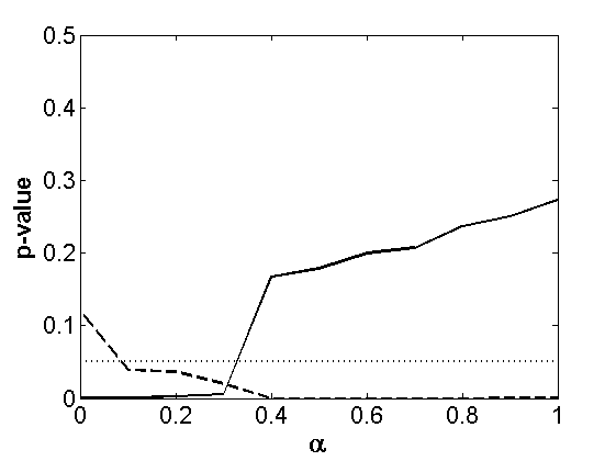
We apply our proposed MDPDE based Wald-type tests for testing the significance of the coefficients of age and the interaction effects to see if the correct inference can be obtained even in the presence of outliers. The resulting p-values are plotted over in Figure 5. Clearly, the classical Wald test (at ) provides incorrect inference at the 5% level in indicating the significance of the age effect and insignificance of the interaction effect between the treatment and the baseline seizure rate. However, our proposed Wald-type tests with positive values of , approximately in the range 0.3 and above, again provide robust (correct) inference under data contamination indicating a significant effect of the interaction between the treatment and the baseline seizure rate on the number of epilepsy attack of a patient along with insignificant effect of patient’s age. This again illustrates the applicability and advantages of our proposal in getting stable and correct insights from any real-life dataset even in the presence of possible outliers in the data.
8 Conclusion and discussions
The class of generalized linear models represents a very important component of the statistical methodology toolbox. In this paper we have dealt with robust tests for testing any general composite null hypothesis in the generalized linear models under the stochastic covariate set up. For this purpose, the family of density power divergences have been utilized; this results in a collection of Wald-type tests which includes the classical Wald test as a special case, but also accommodates other, more robust solutions, some of which attain a very high degree of robustness with little loss in power relative to the classical Wald test for the pure data scenario. The asymptotic properties of these tests and their theoretical robustness have been rigorously established. We have chosen the Poisson regression model for analyzing count data as the medium of demonstration; numerical results illustrating the performances in terms of level and power under different scenarios and graphical results illustrating the nature and behavior of the influence functions clearly establish the usefulness of our proposed tests.
It is important to note that the proposed test directly depends on the MDPDE and so some comments about its computation is needed here. Clearly, the loss function of MDPDEs may have several local minima and hence the corresponding estimating equation may have more than one solution. So, in order to obtain the global minimizer as the MDPDE for general data applications, it is necessary to try different starting values of the optimization algorithm and choose the solution having minimum value of the DPD loss function; these often help to find the absolute minimum with a certain probability depending on the number and structure of the starting parameter values used. This is one advantage of the MDPDE over general M-estimators defined only in terms of estimating equations, since there may not be a easy way to choose from the multiple roots of those estimating equations. However, there is still the requirement of more research and discussion on the computation of the MDPDE as well as in terms of obtaining an efficient algorithms for the same purpose, since the choice of starting values is not clear and may be time consuming. We hope to consider such computational aspects further in our future work.
As we have mentioned briefly in Section 2.2, our present work examines the robustness of the proposed estimators and tests of hypotheses theoretically in terms of boundedness of influence function, which indeed only guarantees their local B-robustness. We have provided empirical illustrations for the influence function and the contamination bias for finite sample illustrations. However, there are several other robustness measures defined from different perspective, including breakdown point, V-robustness etc., which are as crucial in examining the robustness properties. We have provided some limited illustrations of the breakdown property in our numerical illustrations. It would, however, be an interesting future work to verify these measures (including breakdown) theoretically for our MDPDE and the associated Wald-type tests. This would also represent an interesting future work.
Finally, we emphasize again that this work investigated the robustness of the proposed MDPDE and Wald-type tests against data contamination (e.g., outliers). It would be important to investigate the robustness of these procedures in other aspects as well, e.g., against misspecification of the model or the design matrix or any other assumptions including the linearity of the covariates within the GLM. It can be intuitively said that wrongly specifying the design matrix to be fixed while it is random would have the similar effects on the MDPDE as well as on the MLE described in the introduction. On the other hand, since these present MDPDE based methods are developed with particular focus on data contamination, other non-parametric procedures might outperform them in case of a complete misspecification of the underlying model. However, more research is surely needed to examine the extent of model misspecification that our MDPDE can tolerate which we hope to consider in a sequel paper.
Acknowledgments:
We would like to thank two anonymous referees for their helpful comments and suggestions which have improved the paper.
This research has been partially supported by Grant PGC2018-095194-B-100 from Ministerio de Ciencia, Innovacion y Universidades (Spanish government).
The work of AG is also partially supported by the INSPIRE Faculty research grant from Department of Science and Technology, Government of India.
References
- [1] Agresti, A. (2018). An introduction to categorical data analysis. John Wiley & Sons.
- [2] Aeberhard WH, Cantoni E, Heritier S (2014). Robust inference in the negative binomial regression model with an application to falls data. Biometrics, 70, 920-931.
- [3] Anderson, T. W. (2003). An Introduction to Multivariate Statistical Analysis. John Wiley & sons.
- [4] Basu, A., Ghosh, A., Mandal, A., Martin, A., and Pardo, L. (2016). A Wald-type test statistic for testing linear hypothesis in logistic regression models based on minimum density power divergence estimator, Electronic Journal of Statistics, 11 (2), 2741-2772.
- [5] Bianco, A. M., Boent, G., and Rodrigues, I. M. (2013). Robust tests in generalized linear models with missing responses, Computational Statistics and Data Analysis, 65, 80-97.
- [6] Bianco, A. M. and Yohai, V. J. (1996) Robust estimation in the logistic regression model. In Robust statistics, data analysis, and computer intensive methods (Schloss Thurnau, 1994), volume 109 of Lecture Notes in Statist., pp. 17–34. New York: Springer.
- [7] Cantoni, E. and Ronchetti, E. (2001) Robust inference for generalized linear models. Journal of the American Statistical Association, 96, 1022–1030.
- [8] Croux, C. and Haesbroeck, G. (2003) Implementing the Bianco and Yohai estimator for logistic regression. Computational Statistics and Data Analysis, 44, 273–295. Special issue in honour of Stan Azen: a birthday celebration.
- [9] Ghosh, A. and Basu, A. (2016). Robust estimation in generalized linear models: the density power divergence approach, TEST, 25, 269-290.
- [10] Ghosh, A., Mandal, A., Martin, N. and Pardo, L. (2016). Influence Analysis of Robust Wald-type Tests. Journal of Multivariate Analysis, 147, 102–126.
- [11] Hampel, F. R., Ronchetti, E. M., Rousseeuw, P. J., and Stahel, W. A., (1986). Robust statistics: The approach based on influence functions. Wiley Series in Probability and Mathematical Statistics: Probability and Mathematical Statistics. John Wiley & Sons, Inc., New York.
- [12] Krasker, W. S. and Welsch, R. E. (1982) Efficient bounded-influence regression estimation. Journal of the American Statistical Association, 77, 595–604.
- [13] Künsch, H. R., Stefanski, L. A. and Carroll, R. J. (1989) Conditionally unbiased bounded-influence estimation in general regression models, with applications to generalized linear models. Journal of the American Statistical Association, 84, 460–466.
- [14] Leppik IE et al (1985) A double-blind crossover evaluation of progabide in partial seizures. Neurology 35:285
- [15] Marazzi A, Valdora M, Yohai V, Amiguet M (2019). A robust conditional maximum likelihood estimator for generalized linear models with a dispersion parameter. TEST, 28(1), 223–241.
- [16] Maronna, R.A.R.D., Martin, R.D. and Yohai, V. (2006) Robust statistics. Chichester: John Wiley & Sons.
- [17] McCullagh, P. and Nelder, J. A. (1983) Generalized linear models. Monographs on Statistics and Applied Probability. London: Chapman & Hall.
- [18] Morgenthaler, S. (1992) Least-absolute-deviations fits for generalized linear models. Biometrika, 79, 747–754
- [19] Nelder, J. A. and Wedderburn, R. W. M. (1972) Generalized linear models. Journal of the Royal Statistical Society, 135, 370–384
- [20] Rousseeuw, P. J. and Ronchetti, E. (1979) The influence curve for tests. Research Report 21, Fachgruppe fur Statistik, ETH Zurich.
- [21] Stefanski, L. A., Carroll, R. J. and Ruppert, D. (1986a) Optimally bounded score functions for generalized linear models with applications to logistic regression. Biometrika, 73, 413–424.
- [22] Thall PF, Vail SC (1990) Some covariance models for longitudinal count data with overdispersion. Biometrics 46(3):657–671
- [23] Toma, A. and Broniatowski, M. (2011). Dual divergence estimators and tests: Robustness results. Journal of Multivariate Analysis 102(1), 20–36.
- [24] Valdora, M. and Yohai, V. J. (2014). Robust estimators for generalized linear models. Journal of Statistical Planning and Inference, 146, 31-48.