FITspec: a new algorithm for the automated fit of synthetic stellar spectra for OB stars

Abstract

In this paper we describe the FITspec code, a data mining tool for the automatic fitting of synthetic stellar spectra. The program uses a database of 27 000 cmfgen models of stellar atmospheres arranged in a six-dimensional (6D) space, where each dimension corresponds to one model parameter. From these models a library of 2 835 000 synthetic spectra were generated covering the ultraviolet, optical, and infrared region of the electromagnetic spectrum. Using FITspec we adjust the effective temperature and the surface gravity. From the 6D array we also get the luminosity, the metallicity, and three parameters for the stellar wind: the terminal velocity ($v_{\infty}$), the $\beta$ exponent of the velocity law, and the clumping filling factor ($F_{\rm cl}$). Finally, the projected rotational velocity ($v\cdot\sin i$) can be obtained from the library of stellar spectra. Validation of the algorithm was performed by analyzing the spectra of a sample of eight O-type stars taken from the iacob spectroscopic survey of Northern Galactic OB stars. The spectral lines used for the adjustment of the analyzed stars are reproduced with good accuracy. In particular, the effective temperatures calculated with the FITspec are in good agreement with those derived from spectral type and other calibrations for the same stars. The stellar luminosities and projected rotational velocities are also in good agreement with previous quantitative spectroscopic analyses in the literature. An important advantage of FITspec over traditional codes is that the time required for spectral analyses is reduced from months to a few hours.

1 Introduction

The self-consistent analysis of spectral regions from the ultraviolet (UV) to the infrared (IR) radiation band has been made possible because of the large amount of publicly available data combined with the existence of sophisticated stellar atmosphere codes such as cmfgen (Hillier & Miller, 1998), tlusty (Hubeny & Lanz, 1995), and fastwind (Santolaya-Rey et al., 1997; Puls et al., 2005). As a result of this, significant advances have been made toward understanding the physical conditions prevailing in the atmospheres and winds of massive stars. For instance, Fullerton et al. (2000) showed that there were inconsistencies in the optical effective temperature scale in the early far-UV spectra when compared with the scale implied by the observed wind ionization. On the other hand, studies conducted by Martins et al. (2002) and Martins & Schaerer (2003) have shown that the neglect of line blanketing in the models leads to a systematic overestimate of the effective temperature when derived from optical H and He lines. An improvement over these previous calibrations was reported by Martins et al. (2005), where a detailed treatment of non-LTE line-blanketing in the expanding atmospheres of massive stars was taken into account. After direct comparison to earlier calibrations of Vacca et al. (1996), they found effective temperature scales of dwarfs, giants, and supergiants that were lower from 2000 to 8000 K, with the reduction of temperature being the largest for the earliest spectral types and for supergiants. The luminosities were also reduced by 0.20 to 0.35 dex for dwarfs, about 0.25 dex for all giants, and by 0.25 to 0.35 dex for supergiants, with these reductions being almost independent of spectral type for the latter two cases. A more recent analysis by Martins et al. (2015), using the cmfgen code with line-blanketing included, found effective temperatures of Galactic O stars that were in good agreement with the fastwind values reported by Simón-Díaz & Herrero (2014) and Simón-Díaz et al. (2017). On the other hand, Crowther et al. (2002), Hillier et al. (2003), and Bouret et al. (2003) have simultaneously performed analyses of $FUSE$, $HST$, and optical spectra of O-type stars and were able to derive consistent effective temperatures using a wide variety of diagnostics.

A further important result was the recognition of the effects of wind inhomogeneities (i.e., clumping) on the spectral analyses of O-type stars. For instance, Crowther et al. (2002) and Hillier et al. (2003) were unable to reproduce the observed $\mathrm{P}\;$V $\lambda\lambda$1118-1128 profiles when using mass-loss rates derived from the analysis of H$\alpha$ lines. The only way the $\mathrm{P}\;$V and H$\alpha$ profile discrepancies could be resolved was by either assuming substantial clumping or using unrealistically low phosphorus abundances. Therefore, as a consequence of clumping, the mass-loss rates have been lowered by factors ranging from $\sim 3$ to 10. Moreover, new observational clues to understand macroturbulent broadening in massive O- and B-type stars have been provided by Simón-Díaz et al. (2017). They found that the whole O-type and B supergiant domain is dominated by massive stars ($M_{\rm ZAMS}\gtrsim 15$ M_⊙) with a remarkable non-rotational line broadening component, which has been suggested to be a spectroscopic signature of the presence of stellar oscillations in those stars.

Conduction of the above investigations with the aid of any of the existing stellar atmosphere codes is by no means a simple task. Running these codes and performing reliable analyses and calibrations demand a lot of experience that unfortunately many researchers may have no time to acquire. On the other hand, for each interpolation, several models need to be ran, which takes a long time. Thus, the program for fitting atmospheric parameters spends most of its time with this. Therefore, it is desirable to optimize the calculation by developing databases of pre-calculated models as well as the tools that are necessary for their use. Such databases will allow astronomers to save time and analyze stellar atmospheres with reasonable accuracy and without the need of running time consuming simulations. Furthermore, these databases will also speed up the study of a large number of observed spectra that are still waiting for analysis.

The basic parameters of such databases of pre-calculated models are: the surface temperature ($T_{\rm eff}$), the stellar mass ($M$), and the surface chemical composition. However, an adequate analysis of massive stars must also take into account the parameters associated with the stellar wind, such as the terminal velocity ($v_{\infty}$), or the mass-loss rate ($\dot{M}$), and the line clumping. If we take into account the variations of all necessary parameters, the number of pre-calculated models that are actually needed will increase exponentially. Therefore, production of such databases is only possible through the use of supercomputers.

At present, there are a few databases of synthetic stellar spectra available and only with a few tens or hundreds of stellar models (see, for example, Fierro et al. (2015), or the pollux database (Palacios et al., 2010)). To improve on this we have developed a database with tens of thousands of stellar models (Zsargó et al., 2017), which we will release for public use in a short time. Since it is impossible to manually compare an observed spectrum with such an amount of models, it is imperative to develop appropriate tools that allow the automation of this process without compromising the quality of the fitting. With this in mind, we have created FITspec, which is a program that searches in our database for the model that better fits the observed spectrum in the optical. This program uses the Balmer lines to measure the surface gravity ($\log g$) and the line ratios $\mathrm{He}\;$II/$\mathrm{He}\;$I to estimate $T_{\rm eff}$. The paper is organized as follows. In §2, we describe the grid and the six-dimensional (6D) parameter space of the model database. In §3, we give a detailed description of the algorithm and in §4, we test the algorithm by analyzing the spectra of a sample of eight O-type stars taken from the iacob spectroscopic database of Northern Galactic OB stars. Finally, in §5 we summarize the main conclusions.

2 Model database in a six-dimensional parameter space

The stellar models are calculated using the more sophisticated and widely used non-LTE stellar atmosphere code cmfgen (Hillier & Miller, 1998). The code calculates the full spectrum and has been used successfully to model OB stars, W-R stars, luminous blue variables, and even supernovae. It determines the temperature, the ionization structure, and the level populations for all elements in the stellar atmosphere and wind. It solves the radiative transfer equations in the co-moving frame in conjunction with the statistical and radiative equilibrium equations under the assumption of spherical symmetry. The hydrostatic structure can be computed below the sonic point, thereby allowing for the simultaneous treatment of spectral lines formed in the atmosphere, the stellar wind, and the transition region between the two. In particular, the code is well suited for the study of massive OB stars with winds.

At present, our database contains 27 000 atmosphere models, arranged in a 6D space. When all parameter combinations are taken into account, we then expect to have 80 000 models. Each dimension in 6D space corresponds to one parameter of the model. In addition to the surface temperature ($T_{\rm eff}$), the luminosity ($L$), and the metallicity ($Z$) of the star, we consider three more parameters for the stellar wind, namely the terminal velocity ($v_{\infty}$), the $\beta$ exponent of the velocity law, and the clumping filling factor ($F_{\rm cl}$). Here by $v_{\infty}$ we mean the velocity of the stellar wind at a large distance from the star. Outside the photosphere, we model the wind velocity as a function of the stellar radius using the $\beta$-type law (Cassinelli & Olson, 1979), i.e.

$$v(r)=v_{\infty}\left(1-\frac{r}{R_{\star}}\right)^{\beta},$$ (1)

where the free parameter $\beta$ controls how the stellar wind is accelerated to reach the terminal velocity. Low values of $\beta$ (i.e., $\beta=0.8$) indicate a fast wind acceleration, while high values (i.e., $\beta=2.3$) indicate lower accelerations. Since the stellar wind is not necessarily homogeneous, we assume that it contains gas in the form of small clumps or condensations. The volume filling factor $F_{\rm cl}$ is then the fraction of the total volumen occupied by the gas clumps, while the space between them is assumed to be a vacuum. In addition, the mass-loss rate that is used for the models is taken from the evolutionary tracks of Ekström et al. (2012).

In Table 1 we list the values of the relevant model parameters. However, not all of them are truly free parameters. For instance, some of them are associated to other parameters (i.e., the mass loss rate, $\dot{M}$, is completely determined when $T_{\rm eff}$, log g, and $Z$ are known, while $R$ and log g  depend on $M$ and $L$). The dependence of other parameters such as $\beta$ and $F_{\rm cl}$ has not been sufficiently explored and so they could be degenerate with other parameters. For each model, we calculate the synthetic spectra in the UV (900-3 500 Å), optical (3 500-7 500 Å), and near IR (7 500-30 000 Å) radiation bands. In order to facilitate comparison with the observations, the synthetic spectra are rotationally broadened using the program rotin3 (Hubeny & Lanz, 1995), with rotational velocities between 10 and 350 km s^-1 separated by intervals of 10 km s^-1. These discrete values result in a library of 27 000 models $\times$ 3 bands $\times$ 35 values of the rotational velocity $=$ 2 835 000 synthetic spectra. The main parameters of any model atmosphere are the luminosity ($L$) and the effective temperature ($T_{\rm eff}$) from which we can determine the location of the star in the H-R diagram. As appropriate constraints to the input parameters, we use the evolutionary tracks of Ekström et al. (2012) calculated with solar metallicity ($Z=0.014$) at the zero age of the main sequence (ZAMS). Each point of a track corresponds to a star with specific values of $T_{\rm eff}$, luminosity ($L$), and stellar mass (M). We have calculated several models along each track at approximate discrete intervals of 2 500 K in $T_{\rm eff}$. With this provision, the stellar radius, $R$, and the surface gravity, log g, were calculated to determine the luminosity, L, and the stellar mass, M, corresponding to the track. The terminal velocities of the O-type stars in our sample are fitted by $v_{\infty}=2.1v_{\rm esc}$, where $v_{\rm esc}$ is the photospheric escape velocity. The chemical elements that are taken into account in our models are H, He, C, N, O, Si, P, S, and Fe. In particular, the values of the first five elements are taken from Ekström et al. (2012), while for consistency we take the solar metallicity reported by Asplund et al. (2009) for Si, P, S, and Fe in all models.

The code cmfgen employs the concept of “super levels” for the atomic models, where levels of similar energy are grouped together and treated as a single level in the statistical equilibrium equations (see Hillier & Miller, 1998, and references therein). The stellar models in this project include 28 explicit ions of the different elements as a function of their $T_{\rm eff}$. Table 2 summarizes the levels and super levels that are included in the models. The atomic data references are given in the appendix of Herald & Bianchi (2004).

3 The FITspec Algorithm

An experienced astronomer can make a qualitative fit by comparing by eye one or more models with the observed spectrum. However, this procedure becomes too cumbersome and time consuming if hundreds of models must be compared. Also, when the number of models is too large, the objectivity can be easily compromised. FITspec is a heuristic tool that mimics the procedure followed by an experienced astronomer to analyze observed stellar spectra. Due to the big size of the database, it is basically impossible to manually compare the observed spectra with the available models and find the best fit. For this purpose we have developed FITspec, which was also designed to perform this task in a much shorter time compared to traditional fitting algorithms. The usual method to estimate $T_{\rm eff}$ in stellar atmospheres is to compare the equivalent widths (EW) of two lines of the same element in consecutive states of ionization. We have adopted four EW ratios of $\mathrm{He}\;$II and $\mathrm{He}\;$I lines to estimate $T_{\rm eff}$, namely

$$\frac{EW(HeII\,\lambda 4541)}{EW(HeI\,\lambda 4471)}\;(a),\;\;\;\frac{EW(HeII\,\lambda 4200)}{EW(HeI\,\lambda 4026)}\;(b),\;\;\;\frac{EW(HeII\,\lambda 4200)}{EW(HeI\,\lambda 4144)}\;(c),\;\;\;\frac{EW(HeII\,\lambda 4541)}{EW(HeI\,\lambda 4387)}\;(d).$$ (2)

For comparison, Walborn & Fitzpatrick (1990) used the ratios 2(a) and (b) to classify O3-B0 main sequence stars, while the ratios 2(c) and (d) were suitable only for the classification of the later types in the same range. In contrast, we have recorded these ratios for all models in our database. To use FITspec, the user must provide the observed EW of $\mathrm{He}\;$II $\lambda\lambda$ 4541, 4200; $\mathrm{He}\;$I $\lambda\lambda$ 4471, 4387, 4144; and $\mathrm{He}\;$I+$\mathrm{He}\;$II $\lambda\lambda$ 4026 as input data. These values can be easily measured by any astronomical software as, for example, iraf. The algorithm then calculates the EW ratios for the observed lines and compares them with those for the models in the database.

Under the assumption that the best fit model is the one that accurately reproduces the ratios for the observed spectrum, we can calculate the differences between the observed ratios and those pertaining to each model in terms of the relative error

$$Error\left(\frac{\mathrm{He}\;{\small\rm{II}}}{\mathrm{He}\;{\small\rm{I}}}\right)=\frac{\left(\frac{\mathrm{He}\;{\small\rm{II}}}{\mathrm{He}\;{\small\rm{I}}}\right)_{\rm obs}-\left(\frac{\mathrm{He}\;{\small\rm{II}}}{\mathrm{He}\;{\small\rm{I}}}\right)_{\rm mod}}{\left(\frac{\mathrm{He}\;{\small\rm{II}}}{\mathrm{He}\;{\small\rm{I}}}\right)_{\rm obs}},$$ (3)

where $\left(\mathrm{He}\;{\small\rm{II}}/\mathrm{He}\;{\small\rm{I}}\right)_{\rm obs}$ is any of the ratios calculated from the observed spectrum and $\left(\mathrm{He}\;{\small\rm{II}}/\mathrm{He}\;{\small\rm{I}}\right)_{\rm mod}$ is the corresponding ratio for a model. The metric defined by Eq. (3) provides a good measure of the difference between model and observation.

FITspec then calculates a weighted average of the errors in the four ratios considered. The weight of each ratio is an input parameter and must be provided by the user. The program was designed to find all models with average errors less than 50%, save the description of these models in an output file, and produce a graphical output to visualize the location of the models in the 6D parameter space (see Fig. 1). The next step consists of estimating the surface gravity, $\log g$. For this purpose the EWs of the $\mathrm{H}\;$I Balmer lines are used. The errors in the EWs of the six Balmer lines ($\lambda\lambda$3835, 3889, 3970, 4102, 4341, 4861) are then calculated, which are finally used to estimate the $\log g$ of the star. As for the spectral type - effective temperature (SpT - $T_{\rm eff}$) calibration, these errors are calculated using the metric

$$Error_{\rm EW}=\frac{EW_{\rm obs}-EW_{\rm mod}}{EW_{\rm obs}}$$ (4)

where $Error_{\rm EW}$ indicates how different a model and the observation are for a specific line. FITspec also calculates the weighted averages of the relative errors in the EWs of the Balmer lines where the weights must be provided by the user. The algorithm first finds out the models that are within an error of 50% and then picks those models that have both $Error(\mathrm{He}\;{\small\rm{II}}/\mathrm{He}\;{\small\rm{I}})$ and $Error_{\rm EW}$ less than 50%. The total error is calculated according to

$$Error_{\rm tot}=\sqrt{\left(Error_{\rm EW}\right)^{2}+\left[Error\left(\frac{\mathrm{He}\;{\small\rm{II}}}{\mathrm{He}\;{\small\rm{I}}}\right)\right]^{2}}.$$ (5)

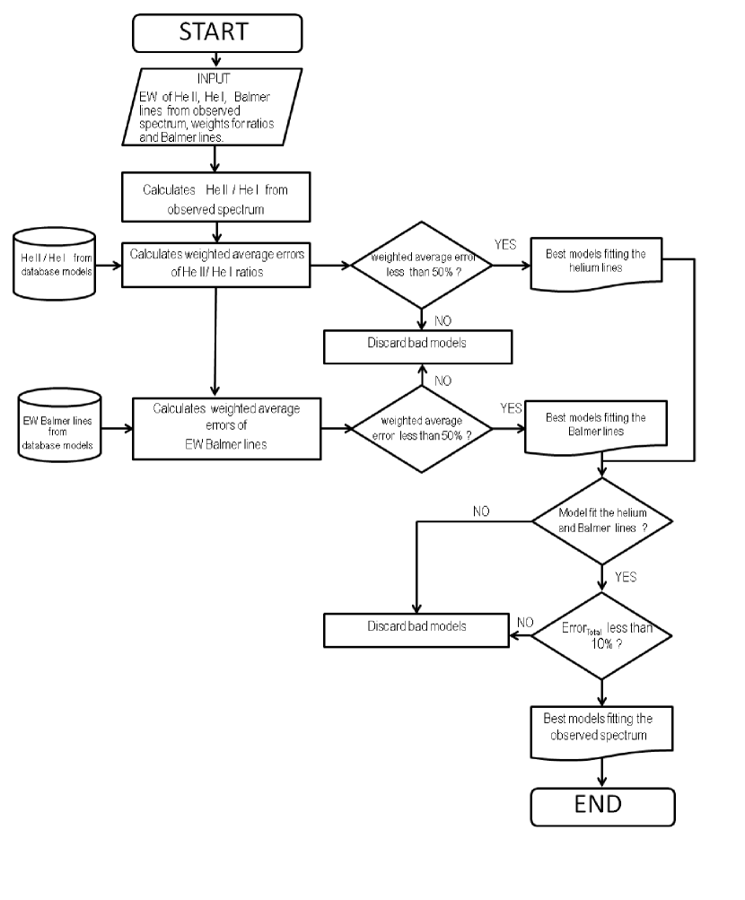
Figure 3: Flowchart showing the sequence of steps followed by the FITspec algorithm.

Finally, the program sorts the errors from lowest to highest values of $Error_{\rm tot}$ and generates a file containing only those models whose total error is less than 10% (see Fig. 2). The sequence of steps followed by FITspec is shown in the flowchart of Fig. 3.

4 Results and discussion

Validation of FITspec is made by testing the algorithm for a sample of eight O-type main-sequence stars. These stars were chosen on the basis of having known available observational data and spectral classification in the iacob database (Simón-Díaz et al., 2011). In addition, they are located in a region of the H-R diagram where our database has the highest density of models. Table 3 lists the stellar parameters as obtained from the best fitted models as found by FITspec for each selected star in our sample. Uncertainties in the effective temperature and luminosity are 1 kK and 0.15 dex, respectively, for all models in the sample. This uncertainties were estimated from the models themeselves. The errors in $T_{\rm eff}$ take into account the models that fit reasonably well the EWs of the He I and He II lines in a global way, while the errors in $L$ include the models that fit reasonably well the EWs of the Balmer lines in a global way. In addition, the first and second columns of Table 4 list the selected stars and their spectral type, respectively, while the next eight columns compare their effective temperatures, surface gravities, and luminosities (also listed in Table 3) with the corresponding values from spectral type calibrations and other spectral analyses reported in the literature. Finally, the last two columns in Table 4 compare the projected rotational velocities as found by FITspec with the corresponding values obtained from several other spectral calibrations, as indicated by the references listed in the footnote of Table 4.

In passing, we note that star HD54662 is a peculiar object. Some authors have treated it as if it were a single star (Markova et al., 2004; Krticka & Kubat, 2010), although there is enough evidence that it is actually a binary star (Fullerton, 1990; Sana et al., 2014; Mossoux et al., 2018). However, in this work HD54662 was taken as a single star because the spectrum extracted from the iacob database shows no evidence of binarity. The corner plots of Figure 1 show the distribution in the 6D space of the models with relative errors less than 50% in the He II/He I ratios for star HD54662 of spectral type O7 V, while Fig. 2 shows the distribution of the models when $Error_{\rm tot}\lesssim 10$% for the same star. When only the temperature criterion is considered, the models span a finite range of values of the parameter space. That is, for prescribed values of the metallicity, filling factor, and $\beta$ exponent of the velocity law, the effective temperature and luminosity of the star can have different values over a finite range. However, when the more stringent criterion $Error_{\rm tot}\lesssim 10$% is applied, the effective temperature and luminosity, vary over very narrow intervals of values with varying metallicity, filling factor, and $\beta$ exponent as we may see from the first column and last row of frames in Fig. 2.

The effective temperatures $T_{\rm eff}$ from spectral type were calculated using the calibrations of Martins et al. (2005) for O-type stars. A comparison of the numbers in columns 3, 4, and 5 of Table 4 show that, in general, there is good agreement between the effective temperatures derived from FITspec and the values calculated from spectral type and other calibrations. The top plot of Fig. 4 compares the effective temperatures obtained from FITspec (triangles) with the spectral type calibrations (asterisks) and the analyses of Martins et al. (2015) (plus signs) and Simón-Díaz et al. (2017) (squares) for our sample of stars. The error bars measure the uncertainties in $T_{\rm eff}$ for each star in these calibrations. The largest error bar corresponds to a temperature interval of 1.9 kK, while the shortest one corresponds to a length of 1 kK. The mean absolute errors between the $T_{\rm eff}$ data derived from FITspec and the corresponding data from spectral type and from all other calibrations in Table 4 are $\approx 1599$ K and $\approx 2338$ K, respectively. If we compare the FITspec data to the more recent calibrations of Nieva (2013), Martins et al. (2015), and Simón-Díaz et al. (2017) the mean absolute error decreases to $\approx 1946$ K. When the uncertainties associated to the FITspec data are neglected, the sample standard deviation is $\approx 1331$ K, which is comparable to the uncertainty of 1000 K in the FITspec data and the mean absolute deviations from the SpT - $T_{\rm eff}$ calibrations.

A further important validation of the FITspec code is the comparison of the predicted surface gravities with the literature values. Columns 6, 7, and 8 of Table 4 provide such a comparison with the SpT - log g calibrations of Martins et al. (2005) and the results from the spectral analyses of Villamariz & Herrero (2002), Nieva (2013), Martins et al. (2015), and Simón-Díaz et al. (2017). There is also a general good agreement between the FITspec data and the SpT - log g calibrations. When the uncertainties in the FITspec gravities are neglected, the mean absolute error between both sets of values is $\approx 0.18$ dex. Similarly, the absolute deviation between the FITspec gravities and the values listed in column 8 is $\approx 0.14$ dex, showing also a good agreement with other calibrations in the literature. The scatter in the FITspec data leads to a sample standard deviation of $\approx 0.20$ dex, which is above the uncertainty of $\pm 0.12$ dex in the predicted gravities and comparable to the mean absolute error between the FITspec and SpT - log g data. The middle plot of Fig. 4 shows the comparison of the log g values. The error bars depict the uncertainty ($\pm 0.15$ dex) in the FITspec values and the calibrations of Martins et al. (2015).

The luminosities $L$ from spectral type are also calculated using the calibrations of Martins et al. (2005). Columns 9 and 10 of Table 4 compare the luminosities derived from these SpT - $L$ calibrations with those found by FITspec. We may see that the values calculated by FITspec are in very good agreement with those from the spectral type calibrations, with absolute deviations varying from 0.02 to 0.37 dex. This comparison is also displayed in the bottom plot of Fig. 4. The uncertainty in the data as represented by the error bars is 0.15 dex for all stars and both calibrations. The mean absolute error between both $log(L/L_{\odot})$ data sets is $\approx 0.16$ dex, which is very close to the actual uncertainty in the data. The largest deviation from the spectral type luminosities occurs for star HD53975, with an absolute difference of 0.37 dex. In addition, the luminosities calculated by FITspec exhibit a dispersion with a sample standard deviation of $\approx 0.25$ dex, which is almost twice the uncertainty in the FITspec luminosities.

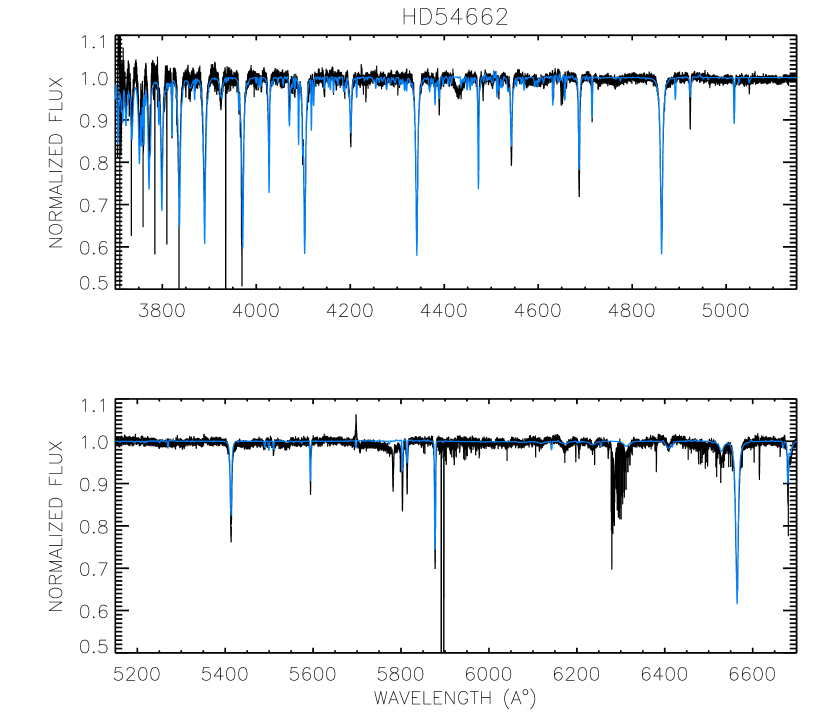
Figure 5: Comparison of the observed spectrum (black line) with that of the best fit model (blue line) for star HD54662.

It is well-known that the rotational broadening of unblended spectral lines changes the line shape but does not affect the EW of the line (Gray, 1992). Therefore, FITspec does not need to apply rotational broadening before the adjustment of the effective temperature and gravity. In fact, this opens the possibility to estimate $v\cdot\sin i$ only with the rotational broadening by adjusting the synthetic spectra to the best fit of the observations, independently of $T_{\rm eff}$ and $\log g$. The last two columns of Table 4 compare the results derived by such adjustments with those from several earlier and more recent analyses. The mean absolute errors between both sets of data is $\approx 19.7$ km s^-1. This reasonable agreement demonstrates the reliability of the results for $v\cdot\sin i$. We may see from Table 4 that if the comparison is made with the more recent calibrations of Oliveira & Hébrard (2006), Nieva (2013), Simón-Díaz & Herrero (2014), Martins et al. (2015), and Simón-Díaz et al. (2017), the mean absolute error increases to $\approx 23.5$ km s^-1. This occurs mainly because of the rather large differences between the FITspec data and the calibrations of Simón-Díaz & Herrero (2014) and Simón-Díaz et al. (2017) for stars HD37022 and HD214680. In this work we have not taken into account the contribution of macroturbulence or any other additional broadening mechanism in the determination of the projected rotational velocities. Any additional broadening mechanism will lower the contribution of rotational broadening for a given observation. In particular, Simón-Díaz et al. (2017) used high-resolution spectra of more than 400 stars with spectral types in the range O4-B9 to provide new empirical clues to explain the occurrence of macroturbulent spectral line broadening in O- and B-type massive stars. They advanced the hypothesis that macroturbulent broadening may be the result of the combined effects of pulsation modes associated with a heat-driven mechanism and possibly-cyclic motions originated by turbulent pressure instabilities, and concluded that the latter mechanism could be the main responsible of the non-rotational line broadening detected in OB stars. While the mechanisms proposed by Simón-Díaz et al. (2017) still lack a definite confirmation, we may argue, based on the comparison between the results of FITspec and the data of Simón-Díaz et al. (2017) for some of the stars in Table 4, that the effects of macroturbulent broadening are in fact those of lowering the projected rotational velocities. Finally, Figs. 5 to 9 compare the observed spectrum (black lines) with that derived from the best fit model (blue lines) for each star of our sample. Most of the salient spectral features are well reproduced by the models, showing the good quality of the fitting obtained by FITspec. Although the results generated by FITspec are reliable, they can be improved by the expert astronomer. In particular, they can be used in analyses where the parameters of a large number of stars are required to be known or as the starting point to make a better adjustment, especially in calibrations related to the chemical composition of the star. In any case, the use of FITspec represents a considerable saving of time compared to other available tools.

The luminosity of a star is directly related to its mass and gravity, which are directly reflected in the Balmer lines. The depth of these lines is in turn reflected into their equivalent width, which is the main criterion employed by FITspec. The use of this criterion has been demonstrated by the goodness of the fit when comparing the effective temperatures and luminosities with those obtained from SpT - $T_{\rm eff}$ and SpT - $L$ calibrations, respectively. In addition, the synthetic spectra of the 6D grid and the FITspec code can be used to adjust observed spectra from a wide variety of telescopes and spectrographs with different resolutions. A method of common use to obtain the best automatic adjustment is to employ a chi-square ($\chi^{2}$) statistics. However, the appropriate use of a $\chi^{2}$ test will degrade the synthetic spectra at the resolution of the observation. Considering that the library of synthetic spectra currently consists of 2 835 000 spectra and that it will certainly continue to grow in number, a suitable comparison using the $\chi^{2}$ statistics involves degrading the synthetic spectra at the same resolution of the observed spectrum. This will also imply the use of additional CPU time. Although this is not a serious problem, it is completely avoided by using the comparison between the EWs and their ratios as the analysis technique. As a final remark, FITspec will be soon available for free download.

5 Conclusions

We have developed and tested the FITspec code, which uses a set of modern automatic tools for searching the best fit models in a database consisting of 27 000 cmfgen model atmospheres. This database will be soon expanded to 80 000 models. The code performs a quantitative spectroscopic analysis of large samples of O- and B-type stars, using objective criteria in a fast and reliable manner compared to traditional calibration tools. It effectively reduces the time needed for the spectral analysis of massive OB stars from months to hours by identifying those models whose $Error_{\rm tot}$ is lower than the allowed tolerance of $\lesssim 10$% and discarding all those models that do not meet this criterion in order to find the effective temperature ($T_{\rm eff}$) and the surface gravity ($\log g$) of a star by fitting the equivalent widths of optical He and $\mathrm{H}\;$I Balmer lines.

The reliability of the algorithm was assessed by analyzing the spectra of eight O-type stars taken from the iacob spectroscopic database of Northern Galactic OB stars and comparing the derived results with those from spectral type - effective temperature (SpT - $T_{\rm eff}$), spectral type - surface gravity (SpT - log g), and spectral type - luminosity (SpT - $L$) calibrations and from previous spectral analysis performed by other authors for the same stars. The values of $T_{\rm eff}$ derived from FITspec are found to match well those calculated from SpT- $T_{\rm eff}$ calibrations and previous analyses from other authors, with mean absolute errors of $\approx 1599$ K and $\approx 2338$ K, respectively. The sample standard deviation of the data generated by FITspec is $\approx 1331$ K, which is well within the range of the mean absolute deviations from the SpT- $T_{\rm eff}$ and other calibrations in the literature. On the other hand, the values of the surface gravity derived by FITspec agree reasonably well with those obtained from SpT -log g calibrations, with a mean absolute error of $\approx 0.18$ dex. A lower absolute deviation of $\approx 0.14$ dex was obtained by comparing with other calibrations. The values of the stellar luminosity derived by the FITspec algorithm were also found to agree with those obtained from the SpT - $L$ calibrations, with a mean absolute error of $\approx 0.16$ dex. This deviation from the SpT - $L$ calibrations is comparable to the uncertainty of 0.15 dex in the FITspec data, which appears to be independent of the spectral type at least for the stars considered in this study.

In order to complement the database of stellar atmosphere models, we have also developed a library of rotationally broadened synthetic spectra, which allows quick estimation of the projected rotational velocity ($v\cdot\sin i$) of a star. The results of the adjustments using this library are also found to agree reasonably well with results from other spectroscopic analyses for the same stars, with a mean absolute error of $\approx 19.7$ km s^-1 when earlier and recent calibrations are taken into account. If the data is compared only with the more recent calibrations, the mean absolute error increases to $\approx 23.5$ km s^-1. The good agreement of the results obtained from FITspec with other spectral analyses demonstrates the reliability of the models.

6 Acknowledgments

We thank the referee for providing a number of valuable comments and suggestions that have improved the content of the manuscript. We acknowledge support from the abacus-Centro de Matemática Aplicada y Cómputo de Alto Rendimiento of Cinvestav-IPN under grant EDOMEX-2011-C01-165873. One of us J.Z. is grateful for support by the CONACyT project CB-2011-01 No. 168632. The calculations of this paper were performed using the abacus computing facilities.

Table 1: Stellar parameters

Parameters in 6D space	Value
$T_{\rm eff}$	from evolutive tracks
$L$	from evolutive tracks
$Z$	solar metallicity and solar metallicity enhanced
	by rotation from evolutive tracks
$v_{\infty}$	2.1$v_{\rm esc}$
$\beta$	0.5, 0.8, 1.1, 1.4, 1.7, 2.1, 2.3
$F_{\rm cl}$	0.05, 0.30, 0.60, 1.00
Other Parameters	Value
$M$	from evolutive tracks
$R$	from $M$ and $L$
log g	from $M$ and $L$
v sin i	from library of synthetic spectra
$\dot{M}$	from evolutive tracks

Table 2: Super levels/levels for the different ionization stages included in the models.

Element	I	II	III	IV	V	VI	VII	VIII
H	20/30	1/1	$\cdots$	$\cdots$	$\cdots$	$\cdots$	$\cdots$	$\cdots$
He	45/69	22/30	1/1	$\cdots$	$\cdots$	$\cdots$	$\cdots$	$\cdots$
C	$\cdots$	40/92	51/84	59/64	1/1	$\cdots$	$\cdots$	$\cdots$
N	$\cdots$	45/85	41/82	44/76	41/49	1/1	$\cdots$	$\cdots$
O	$\cdots$	54/123	88/170	38/78	32/56	25/31	1/1	$\cdots$
Si	$\cdots$	$\cdots$	33/33	22/33	1/1	$\cdots$	$\cdots$	$\cdots$
P	$\cdots$	$\cdots$	$\cdots$	30/90	16/62	1/1	$\cdots$	$\cdots$
S	$\cdots$	$\cdots$	24/44	51/142	31/98	28/58	1/1	$\cdots$
Fe	$\cdots$	$\cdots$	104/1433	74/540	50/220	44/433	29/153	1/1

Table 3: Parameters of the best fit models found by FITspec.

Star	$T_{\rm eff}$	$log(\frac{L}{L_{\odot}})$	$M$	$R$	log g	$Z$	$\dot{M}$	$v_{\infty}$	$F_{\rm cl}$	$\beta$	$v\cdot\sin i$
	(K)		($M_{\odot}$)	($R_{\odot}$)	(cm s-2)		($M_{\odot}$ yr-1)	(km s-1)			(km s-1)
HD34078	33 580$\pm$1000	4.66$\pm$0.15	18.99	43.25	4.120$\pm$0.12	Sun	7.055$\times 10^{-9}$	2 260	0.05	1.1	30
HD36512	31 280$\pm$1000	4.40$\pm$0.15	15.70	37.25	4.168$\pm$0.12	Sun	7.808$\times 10^{-9}$	2 220	0.30	1.7	30
HD36879	32 220$\pm$1000	5.25$\pm$0.15	25.04	91.90	3.572$\pm$0.12	SER	2.063$\times 10^{-7}$	1 770	0.30	0.8	180
HD37022	33 470$\pm$1000	4.91$\pm$0.15	21.66	58.37	3.913$\pm$0.12	SER	7.262$\times 10^{-8}$	2 070	0.60	0.5	100
HD53975	35 030$\pm$1000	4.63$\pm$0.15	19.86	38.76	4.236$\pm$0.12	Sun	6.005$\times 10^{-9}$	2 440	0.05	1.4	160
HD54662	35 500$\pm$1000	4.90$\pm$0.15	22.75	50.65	4.060$\pm$0.12	Sun	1.890$\times 10^{-8}$	2 280	0.05	0.5	80
HD193322	32 460$\pm$1000	4.74$\pm$0.15	19.05	50.67	3.982$\pm$0.12	Sun	2.336$\times 10^{-8}$	2 090	0.30	1.7	50
HD214680	32 980$\pm$1000	4.66$\pm$0.15	18.62	44.97	4.077$\pm$0.12	Sun	1.793$\times 10^{-8}$	2 930	0.30	1.1	40

Table 4: Comparison of parameters found by FITspec with the results of previous calibrations.

Star	SpT	$T_{\rm eff}$	$T_{\rm eff}$	$T_{\rm eff}$	$log\,\textit{g}$	$log\,\textit{g}$	$log\,\textit{g}$	$\log(\frac{L}{L_{\odot}})$	$\log(\frac{L}{L_{\odot}})$	$v\cdot\sin i$	$v\cdot\sin i$
		(K)	(K)	(K)	(cm s-2)	(cm s-2)	(cm s-2)			(km s-1)	(km s-1)
		FITspec	SpT	other	FITspec	SpT	other	FITspec	SpT	FITspec	other
HD34078	O9.5V	33 580$\pm$1000	30 488$\pm$1000	33 000a	4.120$\pm$0.12	3.92	4.0$\pm$0.15a	4.66$\pm$0.15	4.62$\pm$0.15	30	25a
				33 900$\pm$1700b			3.980b				17b
				36 500$\pm$1000c			4.05c				40c
											27f
											13i
HD36512	O9.7V	31 280$\pm$1000	30 000d	32 500a	4.168$\pm$0.12	3.92d	4.0$\pm$0.15a	4.40$\pm$0.15	4.58d	30	20a
				33 900$\pm$1700b			4.210b				15b
				33 400$\pm$ 200e			4.30$\pm$0.05e				20$\pm$2e
							4.13 f				15i
HD36879	O7V	32 220$\pm$1000	35 531$\pm$1000	36 500a	3.572$\pm$0.12	3.92	3.75$\pm$0.15a	5.25$\pm$0.15	5.10$\pm$0.15	180	200a
											200f
											219i
HD37022	O7V	33 470$\pm$1000	35 531$\pm$1000	38 900$\pm$1700b	3.913$\pm$0.12	3.92	4.170b	4.91$\pm$0.15	5.10$\pm$0.15	100	26b
											98f
											26i
HD53975	O7.5V	35 030$\pm$1000	34 419$\pm$1000	35 500$\pm$1900b	4.236$\pm$0.12	3.92	3.590b	4.63$\pm$0.15	5.00$\pm$0.15	160	186b
				36 300h							147f
											163g
											180i
HD54662	O7V	35 500$\pm$1000	35 531$\pm$1000		4.060$\pm$0.12	3.92		4.90$\pm$0.15	5.10$\pm$0.15	80	70f
HD193322	O9V	32 460$\pm$1000	31 524$\pm$1000		3.982$\pm$0.12	3.92		4.74$\pm$0.15	4.72$\pm$0.15	50	94f
											41i
HD214680	O9V	32 980$\pm$1000	31 524$\pm$1000	35 000a	4.077$\pm$0.12	3.92	4.05$\pm$0.15a	4.66$\pm$0.15	4.72$\pm$0.15	40	15a
				35 500$\pm$1900b			3.920b				16b
				37 500$\pm$1000c			4.0c				50c
											32f
											16i

Figure 1: Distribution of the models with errors less than 50% in the six-dimensional (6D) parameter space for star HD54662 of spectral type O7 V. In the first frame of the third row the legend Sun refers to solar metallicity, while SER refers to solar metallicity enhanced by rotation.

Figure 2: Distribution of the best fit models (with errors less than 10%) in the six-dimensional (6D) parameter space for star HD54662. In the first frame of the third row the legend Sun refers to solar metallicity, while SER refers to solar metallicity enhanced by rotation.

Figure 4: (Top panel) Effective temperatures found by FITspec (triangles) compared to the corresponding values obtained from the spectral type (asterisks) and the adjustments of of Martins et al. (2015) (plus signs) and Simón-Díaz et al. (2017) (squares). The largest error bar corresponds to a temperature interval of 1.9 kK, while the shortest one corresponds to a length of 1 kK. (Middle panel) Surface gravity found by FITspec (triangles) compared to the corresponding values obtained from spectral type (asterisks) and the adjustments of Martins et al. (2015) (plus signs) and Simón-Díaz et al. (2017) (squares). The length of the error bars are 0.12 dex for the FITspec data and 0.15 dex for the calibrations of Martins et al. (2015). (Bottom panel) Logarithm of the luminosity found by FITspec (triangles) compared to the corresponding values obtained from the spectral type (asterisks). All error bars correspond to 0.15 dex.

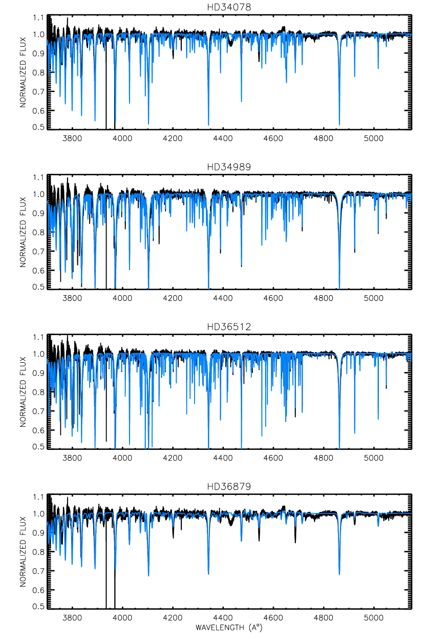
Figure 6: Comparison of the observed spectrum (black line) with that of the best fit model (blue line) for selected sample of stars.

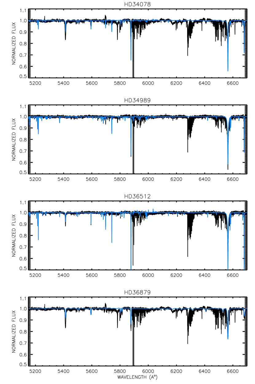
Figure 7: Comparison of the observed spectrum (black line) with that of the best fit model (blue line) for selected sample of stars.

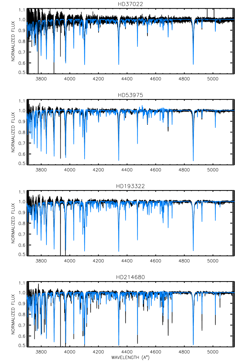
Figure 8: Comparison of the observed spectrum (black line) with that of the best fit model (blue line) for selected sample of stars.

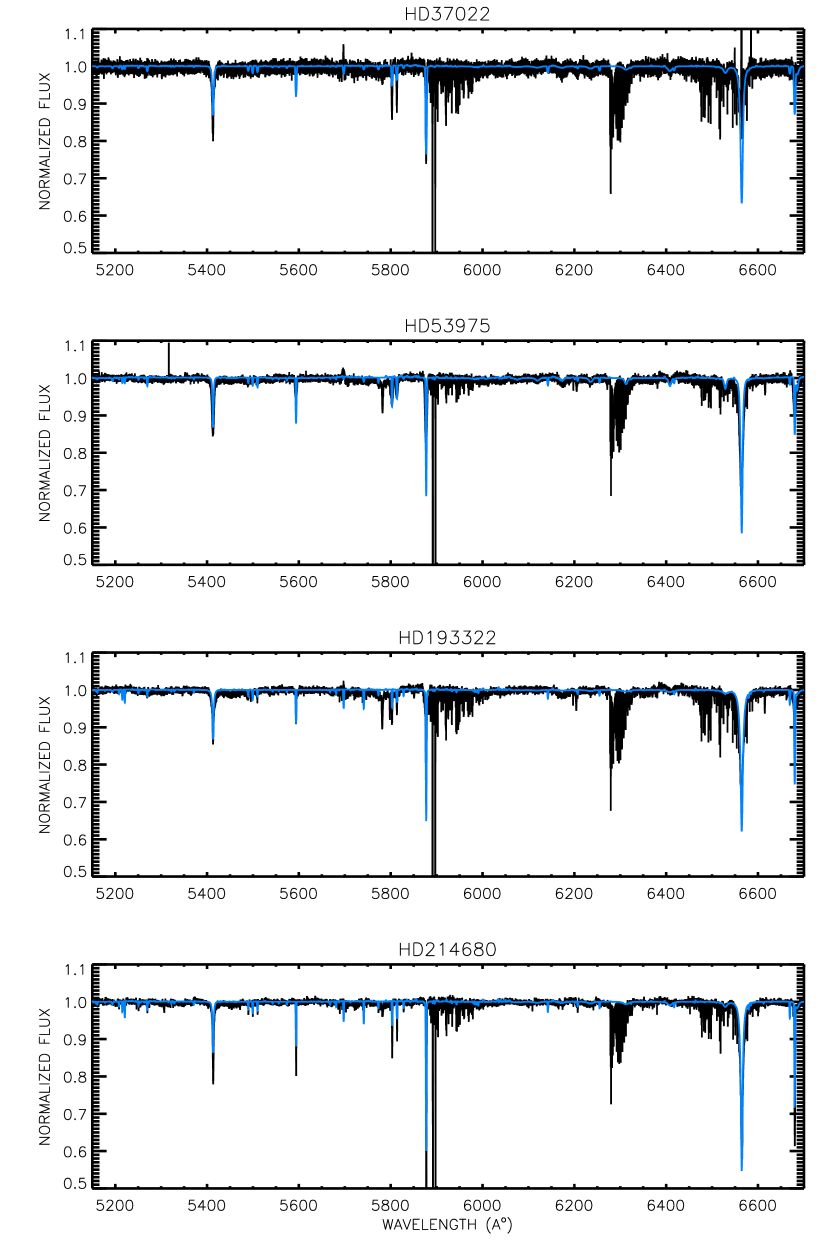
Figure 9: Comparison of the observed spectrum (black line) with that of the best fit model (blue line) for selected sample of stars.

References

- Asplund et al. (2009) Asplund, M., Grevesse, N., Sauval, A. J., & Scott, P. 2009, ARA&A, 47, 481
- Bouret et al. (2003) Bouret, J.-C., Lanz, T., Hillier, D. J., Heap, S. R., Hubeny, I., Lennon, D. J., Smith, L. J., & Evans, C. J. 2003, ApJ, 595, 1182
- Cassinelli & Olson (1979) Cassinelli, J. P. and Olson, G. L. 1979, ApJ, 229, 304
- Conti & Ebbets (1977) Conti, P. S. & Ebbets, D. 1977, ApJ, 213, 438
- Crowther et al. (2002) Crowther, P. A., Hillier, D. J., Evans, C. J., & Fullerton, A. W. 2002, ApJ, 579, 774
- Ekström et al. (2012) Ekström, S., Georgy, C., Eggenberger, P., Meynet, G., Mowlavi, N., Wyttenbach, A., Granada, A., Decressin, T., Hirschi, R., Frischknecht, U., Charbonnel, & Maeder, A. 2012, A&A, 537, A146
- Fierro et al. (2015) Fierro, C. R., Borissova, J., Zsargó, J., Díaz-Azuara, A., Kurtev, R., Georgiev, L., Ramírez-Alegría, S., & Peñaloza, F. 2015, PASP, 127, 428
- Fullerton et al. (2000) Fullerton, A. W., Crowther, P. A., De Marco, O., Hutchings, J. B., Bianchi, L., Brownsberger, K. R., Massa, D. L., Morton, D. C., Rachford, B. L., Snow, T. P., Sonneborn, G., Tumlinson, J., & Willis, A. J. 2000, ApJ, 538, L43
- Fullerton (1990) Fullerton, A. W., 1990, PhD thesis, Toronto Univ. (Ontario).
- Gray (1992) Gray, D. F. 1992. The Observation and Analysis of Stellar Photospheres (Cambridge Astrophysics Series, Vol. 20)
- Herald & Bianchi (2004) Herald, J. E., & Bianchi, L. 2004, ApJ, 609, 378
- Hillier et al. (2003) Hillier, D. J., Lanz, T., Heap, S. R., Hubeny, I., Smith, L. J., Evans, C. J., Lennon, D. J., & Bouret, J. C. 2003, ApJ, 588, 1039
- Hillier & Miller (1998) Hillier, D. J. & Miller, D. L. 1998, ApJ, 496, 407
- Howarth & Prinja (1989) Howarth, I. D. & , Prinja, R. K. 1989, ApJS, 69, 527
- Hubeny & Lanz (1995) Hubeny, I., & Lanz, T. 1995, ApJ, 439, 875
- Krticka & Kubat (2010) Krticka, J., & Kubat, J. 2010, A&A, 519, 50
- Markova et al. (2004) Markova, N., Puls, J. Repolust, T. & Markov, H. 2004, A&A, 413, 693
- Martins & Schaerer (2003) Martins, F. & Schaerer, D. 2003, in Astronomical Society of the Pacific Conference Series, Vol. 288, ed. I. Hubeny, D. Mihalas, & K. Werner (San Francisco: Astronomical Society of the Pacific), 267
- Martins et al. (2002) Martins, F., Schaerer, D., & Hillier, D. J. 2002, A&A, 382, 999
- Martins et al. (2005) Martins, F., Schaerer, D., & Hillier, D. J. 2005, A&A, 436, 1049
- Martins et al. (2015) Martins, F., Hervé, A., & Bouret, J. C. Marcolino, W., Wade, G. A., Neiner, C., Alecian, E., Grunhut, J. and Petit, V., 2015, A&A, 575, A34
- Mossoux et al. (2018) Mossoux, L., Mahy, L., & Rauw, G. 2018, arXiv, 18206535
- Nieva (2013) Nieva, M.-F. 2013, A&A, 550, A26 (14 pp.)
- Oliveira & Hébrard (2006) Oliveira, C. M. & Hébrard, G. 2006, ApJ, 653, 345
- Palacios et al. (2010) Palacios, A., Gebran, M., Josselin, E., Martins, F., Plez, B., Belmas, M., & Lèbre, A. 2010, A&A, 516, A13
- Puls et al. (2005) Puls, J., Urbaneja, M. A., Venero, R., Repolust, T., Springmann, U., Jokuthy, A., & Mokiem M. R. 2005, A&A, 435, 669
- Sana et al. (2014) Sana, H., Le Bouquin, J.-B., Lacour, S., et al. 2014, ApJS, 215, 15
- Santolaya-Rey et al. (1997) Santolaya-Rey, A. E., Puls, J., & Herrero, A. 1997, A&A, 323, 488
- Simón-Díaz et al. (2011) Simón-Díaz, S., Castro, N., Garcia, M., Herrero, A., & Markova, N. 2011, Bulletin de la Société Royale des Sciences de Liège, 80, 514
- Simón-Díaz et al. (2017) Simón-Díaz, S., Godart, M., Castro, N., Herrero, A., Aerts, C., Puls, J., Telting, J. & Grassitelli, L. 2017, A&A, 597, A22 (17 pp.)
- Simón-Díaz & Herrero (2014) Simón-Díaz, S. & Herrero, A. 2014, A&A, 562, A135
- Sybesma & De Loore (1982) Sybesma, C. H. B. & De Loore, C. 1982, A&A, 111, 229
- Vacca et al. (1996) Vacca, W. D., Garmany, C. D., & Shull, J. M. 1996, ApJ, 460, 914
- Villamariz & Herrero (2002) Villamariz, M. R. & Herrero, A. 2002, in Astronomical Society of the Pacific Conference Series, Vol. 274, ed. T. Lejeune & J. Fernandez, 234
- Walborn & Fitzpatrick (1990) Walborn, N. R. and Fitzpatrick, E. L. 1990, PASP, 102, 379
- Zsargó et al. (2017) Zsargó, J., Arrieta, A., Fierro, C., Klapp, J., Hillier, D. J., Arias, L., Mendoza, J., & Georgiev, L. N. 2017, in Astronomical Society of the Pacific Conference Series, Vol. 508. ed. A. Miroshnichenko, S. Zharikov, D. Korčáková, & M. Wolf, 407