Dark Matter Distribution Induced by a Cosmic String Wake in the Nonlinear Regime

Abstract

We study the distribution of dark matter in the nonlinear regime in a model in which the primordial fluctuations include, in addition to the dominant primordial Gaussian fluctuations generated by the standard $\Lambda CDM$ cosmological model, the effects of a cosmic string wake set up at the time of equal matter and radiation, making use of cosmological $N$-body simulations. At early times the string wake leads to a planar overdensity of dark matter. We study how this non-Gaussian pattern of a cosmic string wake evolves in the presence of the Gaussian perturbations, making use of wavelet and ridgelet-like statistics specifically designed to extract string wake signals. At late times the Gaussian fluctuations disrupt the string wake. We find that for a string tension of $G\mu=10^{-7}$, a value just below the current observational limit, the effects of a string wake can be identified in the dark matter distribution, using the current level of the statistical analysis, down to a redshift of $z=10$.

I Introduction

Cosmic strings are linear topological defects which arise in a large class of quantum field theory models describing physics beyond the Standard Model. If Nature is described by such a model, then a network of strings inevitably forms in the early universe and persists to the present time Kibble . Strings are thin lines of trapped energy density and their gravitational effects lead to specific signatures which can be searched for in cosmological observations.

The network of cosmic strings which form in a gauge field theory approaches a scaling solution in which the statistical properties of the distribution of strings is independent of time when all lengths are scaled by the Hubble radius (see e.g. VS ; HK ; RHBCSrev for reviews of cosmic strings and their role in cosmology). The string distribution has two components: firstly a network of infinite strings with mean curvature radius comparable to the Hubble radius $t$ (where $t$ is the physical time), and secondly a distribution of string loops with radii $R<t$. The loops result from the long string intersections which also are responsible for maintaining the long string scaling distribution. Analytical arguments lead to the conclusion that the number $N$ of long string segments that pass through any Hubble volume is of the order $1$. The exact number must be determined in numerical cosmic string evolution simulations (see e.g. CSsimuls for some recent results). Current evidence is that $N\sim 10$.

Cosmic strings are characterized by their mass per unit length $\mu$ which is usually expressed in terms of the dimensionless quantity $G\mu$ (where $G$ is Newton’s gravitational constant ). The value of $\mu$ is determined by the energy scale $\eta$ at which the strings are formed (it is the energy scale of the phase transition leading to the strings)

$$\mu\,\sim\,\eta^{2}\,.$$ (1)

The strength of the signatures of cosmic strings in the sky are proportional to $G\mu$. The current upper bound on the string tension is

$$G\mu\,<\,1.5\times 10^{-7}\,$$ (2)

and is derived from the features of the angular power of cosmic microwave background (CMB) anisotropies Dvorkin ; PlanckCS (see also CMBlimits for some older works). Searching for cosmic strings in the sky hence is a way to probe particle physics beyond the Standard Model “from top down”, as opposed to accelerator searches which are more sensitive to low values of $\eta$ and hence probe particle physics “from bottom up”. The current bound on $G\mu$ already rules out the class of “Grand Unified” particle physics models containing cosmic string solutions with a scale of symmetry breaking which is on the upper end of the preferred range. Improving the upper bound on the cosmic string tension will lead to tighter constraints on particle physics models (see e.g. RHBtopRev for an elaboration on these points).

The long string segments lead to non-Gaussian signals in the sky characterized by specific geometrical signatures in position space maps. One set of string signatures comes from lensing produced by a string. Space perpendicular to a long straight string segment is a cone with deficit angle $\alpha$ given by deficit

$$\alpha\,=\,8\pi G\mu\,.$$ (3)

The deficit angle extends to a distance $t$ from the string Joao . Cosmic strings are relativistic objects and hence the curvature of the string segments (the curvature radius is of the order $t$) will induce relativistic motion of the string in the plane perpendicular to the tangent vector of the string. This will lead to line discontinuities in CMB anisotropy maps KS of magnitude

$$\frac{\delta T}{T}\,=\,4\pi v_{s}\gamma_{s}G\mu\,,$$ (4)

where $v_{s}$ is the transverse speed of the string segment, and $\gamma_{s}$ is the corresponding relativistic gamma factor.

A moving long string segment will also induce a velocity perturbation behind the string towards to plane determined by the tangent vector of the string and the velocity vector. This leads to a region behind the string with twice the background density called a cosmic string wake wake . A wake produced by a string passing through matter at time $t$ will have comoving planar dimensions given by the Hubble radius at time $t$, and a comoving thickness which initially is given by the deficit angle (3) times the Hubble radius and which grows linearly in time as given by the result of an analytical analysis wakegrowth making use of the Zel’dovich approximation Zeld . Hence, the comoving dimensions of a wake produced at time $t$ are

$$c_{1}tz(t)\times tz(t)v_{s}\gamma_{s}\times 4\pi G\mu v_{s}\gamma_{s}z(t)t\,,$$ (5)

where $z(t)$ is the redshift at time $t$, and $c_{1}$ is a constant of order unity which gives the string curvature radius relative to $t$.

According to the cosmic string network scaling solution, strings lead to a set of line discontinuities in CMB temperature maps. The overall distribution of these discontinuities is scale-invariant. However, since cosmic strings are primordial isocurvature fluctuations, they do not give rise to acoustic oscillations in the angular CMB temperature power spectrum, oscillations which are typical of adiabatic perturbations noacoustic . Hence, detailed measurements of the CMB angular power spectrum leads to the constraints on the string tension is given by (2). It is likely that the bound can be strengthened by analyzing CMB temperature maps in position space using statistical methods designed to identify linear discontinuities. Initial studies using the Canny edge detection algorithms Danos , wavelets Hergt ; PlanckCS ; Hiranya , curvelets Hergt and machine learning tools Oscar2 have shown that good angular resolution is key to obtaining improved constaints . Cosmic strings also lead to direct B-mode polarization in the CMB sky Holder1 (see also RHBCSrevNew for a recent review of signatures of cosmic strings in new observational windows) .

Cosmic strings also lead to distinct patterns in 21cm redshift surveys: a cosmic string wake present at a redshift before reionization will lead to a three-dimensional wedge of extra absorption in the 21cm maps because at these redshifts the wake is a region of twice the background density of neutral hydrogen and CMB photons passing through a wake suffer twice the absorption compared to photons which do not pass through the wake Holder2 . Strings also lead to a Wouthuysen-Field brightness trough in the integrated 21cm signal Oscar .

In contrast, there has been little recent work on how well the cosmic string tension can be constrained by the large-scale structure of the Universe at lower redshifts, well into the nonlinear region of gravitational clustering . In this paper we take first steps at studying these signals. We will study how well a single cosmic string wake can be identified in $N$-body dark matter simulations of gravitational clustering.

Specifically, we include the effects of a cosmic string wake in a cosmological $N$-body simulation which evolves the dark matter distribution. We introduce a statistic which is designed to pick out the signal of a cosmic string wake in the “noise” of the primordial Gaussian fluctuations in a $\Lambda CDM$ cosmology. Since the string wake grows only in direction perpendicular to the plane of the wake, whereas the Gaussian fluctuations grow in all three dimensions, the Gaussian fluctuations will eventually disrupt the wake, as studied analytically in us . However, even once the wake has been locally disrupted, its global signal will persist for some time. We study how the redshift when this global signal ceases to be identifiable varies as the string tension changes. In the following, we shall call the Gaussian fluctuations in a $\Lambda CDM$ cosmology simply as “Gaussian noise”.

II Wake Disruption

The challenge of identifying cosmic string wake signals in the nonlinear regime of structure formation was addressed in us . If a cosmic string wake is added to the initial conditions of a cosmological model which is characterized by a scale-invariant spectrum of primordial Gaussian cosmological perturbations, then the wake is clearly identifiable at high redshifts since the Gaussian perturbations are all in the linear regime whereas the wake is already a nonlinear density contrast. However, once the Gaussian perturbations become nonlinear they will start to disrupt the wake.

A first criterion for the stability of a wake is that the local displacement $S_{k}$ of matter on the comoving scale of the wake thickness $k^{-1}(t)$ due to the Gaussian fluctuations be smaller than the physical width of the wake $h(t)$, i.e.

$$S_{k}(t)\,<\,h(t)\,.$$ (6)

If this condition is satisfied, then the wake should persist as a locally coherent entity. This condition was called the local stability condition. A closely related condition is the local delta condition which demands that the mean fluctuation $\Delta$ due to the Gaussian fluctuations on the scale $k$ of the wake thickness be smaller than unity, i.e.

$$\Delta(k,t)\,<\,1\,.$$ (7)

For a string tension of $G\mu=10^{-7}$ it was found that the local delta condition is satisfied down to a redshift of $z\simeq 5$. The limiting redshift increases as the string tension decreases. For $G\mu=10^{-11}$ the limiting redshift is $z\sim 11$, and this limiting redshift increases only slowly as the string tension is reduced further (for a string tension of $G\mu=10^{-14}$ the limiting redshift is $z\sim 20$).

The above result shows that in principle very high redshift surveys of the distribution of matter in the universe such as what can be achieved by high redshift 21cm maps yield a very promising avenue to detect cosmic strings Holder2 . The challenge, however, is to be able to identify the very thin features (in redshift direction) which string wakes will produce.

As was also studied in us , wakes might be identifiable through the global mass distribution which they induce even if they are locally disrupted. We can ask the question whether the Gaussian fluctuations are able to induce a nonlinear overdensity in a box of the expected dimensions of a string wake. The contribution of the Gaussian fluctuations to the variance in a such a box $B(G\mu)$ is

$$\sigma_{w}^{2}\,=\,\frac{g^{2}(z)}{(2\pi)^{3}}\int d^{3}kP(|k|)W_{w}^{2}(k)\,,$$ (8)

where $P(|k|)$ is the power spectrum of the Gaussian noise, $g(z)$ is the cosmological growth factor, and $W_{w}(k)$ is a non-isotropic window function which filters out contributions from modes which have wavelength smaller than the width of the wake in one direction, and smaller than the extent of the wake in the two other dimensions. If $\sigma_{w}<1$, then a string wake can be identified by its global signal (it will produce a nonlinear density contrast in this box). Thus, we can define the global delta condition for the identifiability of a string wake:

$$\sigma_{w}\,<\,1\,.$$ (9)

It was found us that for a roughly scale-invariant power spectrum of primordial fluctuations the result for $\sigma_{w}$ is to first order independent of the thickness of the wake, and that the condition (9) remains satisfied down to redshift $0$. Hence, in the absence of noise and with unlimited resolution a string wake should be identifiable even at the present time for any value of $G\mu$. In practice, however, the limited resolution of a survey (and the limiting resolution of numerical simulations) will limit the redshift range where the string wake can be detected.

The goal of the present study is to determine to what value of $G\mu$ cosmic string wakes can be identified in practice. Ultimately we are interested in comparing the results of numerical simulations of the distribution of matter, obtained if the usual initial conditions for the primordial fluctuations are supplemented with the presence of a cosmic string wake, with observational data. In the current project we will study the distribution of dark matter only. Any observational data set will have a limiting resolution in the same way that any numerical simulation has a resolution limit. These limits will render the effects of string wakes harder and harder to detect the smaller the value of $G\mu$, in spite of the fact that the result (9) is independent of $G\mu$. In this paper we wish to study whether the wake of a string with tension $G\mu=10^{-7}$, a value just below the current upper bound, can be identified with simulations having a resolution which can currently be achieved.

In the next section we describe the simulation code and various performance tests of the code which we have performed. For these test runs we use a value of $G\mu$ which is larger than the current upper bound in order to better visualize the results. In Section 4 we then present the output of runs for values of $G\mu$ down to $G\mu=10^{-7}$, and study down to which redshift the wake signal can be identified with various statistics. In Section 5 we summarize the results and discuss prospects for deriving improved limits.

III Simulations

III.1 The Code

This section describes the main features of the $N$-body simulations that we use to model numerically the wake evolution and its impact on the density field. We detail our wake insertion strategy and validate our results with consistency checks.

The simulations were produced with CUBEP³M, a public high performance cosmological $N$-body code based on a two-level mesh gravity solver augmented with sub-grid particle-particle interactions code . The initial conditions generator reads a transfer function constructed with the CAMB online toolkit and produces $\Lambda$CDM fluctuations at any chosen initial redshift $z_{i}$ with the following cosmological parameter: $\Omega_{\Lambda}=0.7095$, $\Omega_{\rm b}=0.0445$, $\Omega_{\rm CDM}=0.246$, $n_{t}=1$, $n_{s}=0.96$, $\sigma_{8}=0.8628$, $h=0.70$, $T_{\rm cmb}(t_{0})=2.7255$. The initial redshift is chosen such that the initial fluctuations are in the linear regime for all scales that we resolve. Except few cases, the intial redshift was $z_{i}=63$. Particles are then displaced using linear theory Zeld , then evolved with CUBEP³M until redshift $z=0$. Several test simulations were performed with various computational power on four systems: a laptop with 4 processors, a 64 cores computer cluster in the McGill Physics Department called irulan, and a set of 128 cores from the Guillimin Cluster and, finally, a set of 128 cores from the Graham Cluster. The two last clusters are part of the Compute Canada Consortium. The first two set of simulations were launched as a single MPI task jobs, whereas the two last ones were distributed over 8 compute nodes. The cosmological volume and the number of particles were varied, as summarized in Table 1. The most powerful simulation was performed in Graham, in a volume of $L_{\rm box}=64$Mpc/$h$ per side, with $nc$ = 2048 cells per dimension (corresponding to 1024 particles per dimension). The phase space output data was saved for checkpoints chosen in equal spaced logarithmic intervals for the scale factor. In addition to that, a few more checkpoints were added, corresponding in total to the following redshifts: $63,31,15,10,7,5,4,3,2,1,0.5,0$ (some other simulations contain $255$ and $127$ as well).

Machine	$L_{\rm box}$ (in Mpc/$h$)	$nc$
ACER	40	240
irulan	64 and 32	512 and 256
Guillimin	64	1024
Graham	64	1024 and 2048

Table 1: Configuration of the various $N$-body simulations. $L_{\rm box}$ and $nc$ are the side of the cosmological box and number of cells per dimension, respectively.

The $\Lambda CDM$ part of the $N$-body code has been shown to match the predictions to within 5% over a large range of scales. We verify this in Fig. 1, where we compare the matter power spectrum $P(k)$ with the predictions at $z=15$ for a ACER simulation with $L_{\rm box}=40$Mpc/$h$ and $nc=240$. The power spectrum is computed by first assigning the particles onto a density grid $\delta(x)$ using the cloud-in-cell interpolation, then squaring the Fourier transformed field $\delta(k)$ and averaging over the solid angle $\Omega$: $P(k)=\langle|\delta(k)|^{2}\rangle_{\Omega}$. The mass assignment scheme has been removed in this calculation, but the shot noise was not removed, which explains the large rise at $k>10h/{\rm Mpc}$. We observe that the agreement is indeed as expected, with a 10% match for $k<3.0h$/Mpc, corresponding to scales 1.04 Mpc/$h$.

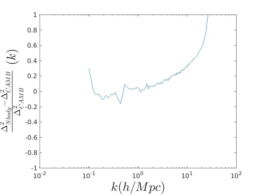
Figure 1: Plot of fractional error of the dimensionless power spectrum compared with the HALOFIT predictions of the online CAMB tool

The reason we cannot achieve $5\%$ precision on $P(k)$ is due to the fact that we do not fully capture the linear scales, because we are considering a small box size. We would normally need $L_{box}>200\ {\rm Mpc}/h$ to get $5\%$ precision on $P(k)$. In our case this is not an issue, since we are still producing representative $\Lambda CDM$ fluctuations from which the wake must be extracted.

III.2 Wake Insertion

One of the goals is to produce particle distributions including the effects of a wake with a cosmic string tension compatible with the current limit of $G\mu=10^{-7}$, which corresponds to a comoving width of $\approx 0.003h^{-1}{\rm Mpc}$ at redshift 20, a redshift in which we have confidence that the wake is not yet locally disrupted us .

For a given simulation without a wake, we evolved two independent simulations corresponding to wake insertions at redshifts $z=31$ and $z=15$ to test the sensibility of the results on the time of wake insertion. The advantage of an early insertion is that the dark matter distribution is in the linear regime. On the other hand a late wake insertion corresponds to a thicker wake at the time of insertion, giving a better resolution of its thickness.

For each configuration, a $\Lambda$CDM-only simulation was evolved to $z=0$, without the wake, writing the particle phase space at a number of redshifts including the wake insertion redshift. We next modified the particle phase space at the wake insertion redshift by displacing the particles and also giving them a velocity kick towards the central plane. The magnitudes of the velocity and displacement are calculated according to the Zel’dovich approximation Zeld .

We consider a wake which was laid down at the time $t_{eq}$ of equal matter and radiation (such wakes are the most numerous and also the thickest). Their comoving planar distance $d$ is given by the comoving horizon at $t_{eq}$, namely

$$d\,=\,z(t_{eq})^{-1/2}t_{0}\,$$ (10)

where $t_{0}$ is the present time. This distance is larger than the size of our simulation box, which justifies inserting the effects of a wake as a planar perturbation. The initial velocity perturbation towards the plane of the wake which the particles receive at $t_{eq}$ is

$$\delta v\,=\,4\pi G\mu v_{s}\gamma_{s}\,,$$ (11)

where $v_{s}$ is the transverse velocity of the string and $\gamma_{s}$ is the corresponding relativistic gamma factor. Since cosmic strings are relativistic objects, we will take $v_{s}\gamma_{s}=1/\sqrt{3}$. In the following equations, however, we leave $v_{s}\gamma_{s}$ general.

The initial velocity perturbation leads to a comoving displacement $\psi(t)$ of particles towards the plane of the wake. This problem was discussed in detail in wakegrowth , with the result that the comoving displacement at times $t>t_{eq}$ is given by

$$\psi(t)\,=\,\frac{3}{5}4\pi G\mu v_{s}\gamma_{s}t_{eq}z(t_{eq})\frac{z(t_{eq})}{z(t)}\,.$$ (12)

The last factor represents the linear theory growth of the fluctuation, the previous factor of $z(t_{eq})$ represents the conversion from physical to comoving velocity. The (comoving) velocity perturbation is

$${\dot{\psi}}(t)\,=\,\frac{2}{5}4\pi G\mu v_{s}\gamma_{s}t_{eq}z(t_{eq})\frac{z(t_{eq})}{z(t)}\frac{1}{t}\,.$$ (13)

In our simulations the displacement and velocity perturbations towards the plane of the wake were given by (12) and (13), respectively, evaluated at the time $t=t_{i}$ of wake insertion. We then reload this modified particle data into CUBEP³M and let the code evolve again to redshift $z=0$. This method ensures that the differences seen in the late time matter fields are caused only by the presence of the wake. The $\Lambda$CDM background is otherwise identical.

To test the wake insertion code, simulations were run with a large cosmic string tension of $G\mu=4.0\times 10^{-6}$. The following three panels each show a two dimensional projection of the resulting dark matter distribution at redshifts $z=31$, $z=10$ and $z=3$. The results are from a Graham simulation with $nc=512$ particles per dimension and a cubic lateral size of $64\ {\rm Mpc}/h$. The initial conditions for the $\Lambda$CDM fluctuations were generated at $z=255$ and a wake was inserted at $z=127$.

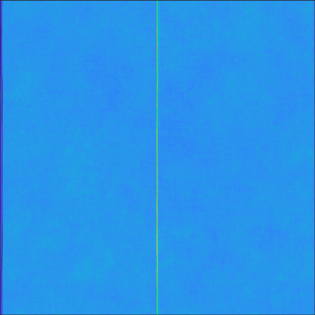
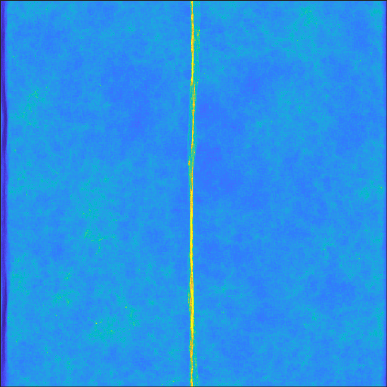
Figure 2: Density contrast of the two dimensional projection of the dark matter distribution for a $G\mu=4.0\times 10^{-6}$ wake at redshift $z=31,10$ and $3$ (from top to bottom, respectively). The color bar on the bottom associates each color with the corresponding density contrast

The first figure shows the completely undistorted initial wake signal. At redshift $z=10$ the wake is no longer perfectly uniform, and at redshift $z=6$ the $\Lambda$CDM fluctuations have caused major inhomogeneities in the wake, and some small deflections. However, for this large string tension the string fluctuations still dominate.

III.3 Known limitations

Our numerical modeling of a string-induced wake has multiple limitations. The first one concerns resolution, and results from the fact that we are not always able to resolve the wake itself, which is increasingly thinner for lower string tensions. Ideally, the thickness of the wake should be at least as large as the simulation cell size, but this is not always feasible to achieve in a cosmological setup, given the computing resources at our disposal. For example, supposing we would like to resolve a wake produced by a cosmic string with tension $G\mu=1.0\times 10^{-7}$ at redshift $z=7$, the grid size needs to be $0.01{\rm Mpc}/h$, which, assuming a large simulation with 8192 cells per dimension, corresponds to a lateral size of $\approx 57\ {\rm Mpc}/h$. We circumvent this computing challenge by noting that the wake has a global impact on the matter field, and that we do not need to resolve the initial wake exactly to detect its presence.

A second, less intuitive, limitation arises from the wake insertion itself: once every particle has been moved towards the wake, a planar region parallel to the wake is left empty at the boundary of the simulation box. In other words, the number of particles in the simulation is fixed, and the dislocation of the particles that is required to create the wake (an overdense region in the central plane of the simulation) produce at the same time an underdense region at the boundary plane. Although there is indeed a compensating underdensity at large distances from the wake (this is required by the “Traschen integral constraints” Traschen on density fluctuations in General Relativity), the fact that the void occurs at the boundary of our simulation box is unphysical. Note, in particular, that in the simulations the location of the underdensity depends on the box size, and it should be pushed to the horizon size at wake formation Joao . In order to preserve the cosmological background in the simulation, we cannot introduce new particles to fill this empty region, and hence we have no way to get rid of this undesired effect.

Our approach is therefore to examine whether or not this void affects the evolution of the wake. We achieve this by measuring the displacement of the particles induced by the presence of the wake (and the corresponding void at the boundary) and comparing the result with the Zel’dovich approximation formula (12). Each particle in the simulation carries an identification number, and so it is possible to compute the position of a particle in a simulation without a wake and compare with the position of the same particle in the simulation that has an inserted wake. Since the only difference between the two simulations is the wake insertion, by subtracting the two positions it is possible to obtain the displacement of this particle induced by the wake.

Figure 3 shows the displacement in the direction perpendicular to the wake induced on the particles by the presence of the wake. A Guillimim simulation with $G\mu=8\times 10^{-7}$, number of cells per dimension $nc=512$ and lateral size $L=64\ {\rm Mpc}/h$ was used and the figure corresponds to $z=10$, with a wake inserted at $z=31$. The axis perpendicular to the wake was divided into bins with the same thickness as the cell size and the displacement associated to a given bin was computed by averaging over the displacements of all the particles inside it. The particles on the left receive a positive dislocation (towards the wake at the center) and the particles on the right side receive a negative displacement towards the wake, as expected.

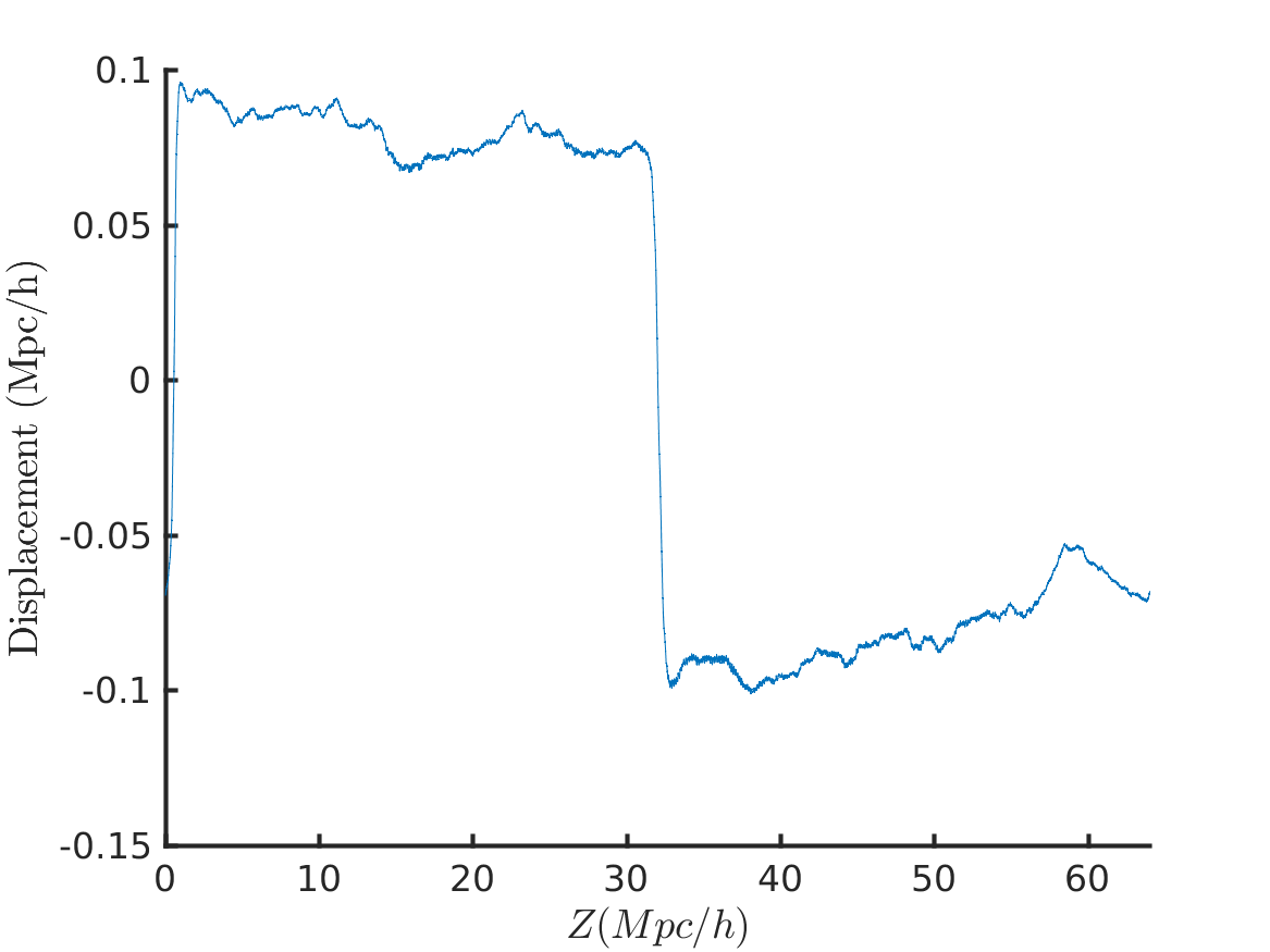
Figure 3: Plot of the induced displacement due to the wake as a function of axis position $Z$ (horizontal axis) for redshift $z=10$ and string tension $G\mu=8\times 10^{-7}$

A number associated to the displacement associated to the above case was computed by considering the mean of the positive part, the absolute value of the mean of the negative part and taking the average of those two quantities. The error associated with this displacement computation was the average of the standard deviation of each part (positive and negative). Figure 4 is a summary of this computation for different redshifts together with the expected result from the Zel’dovich approximation.

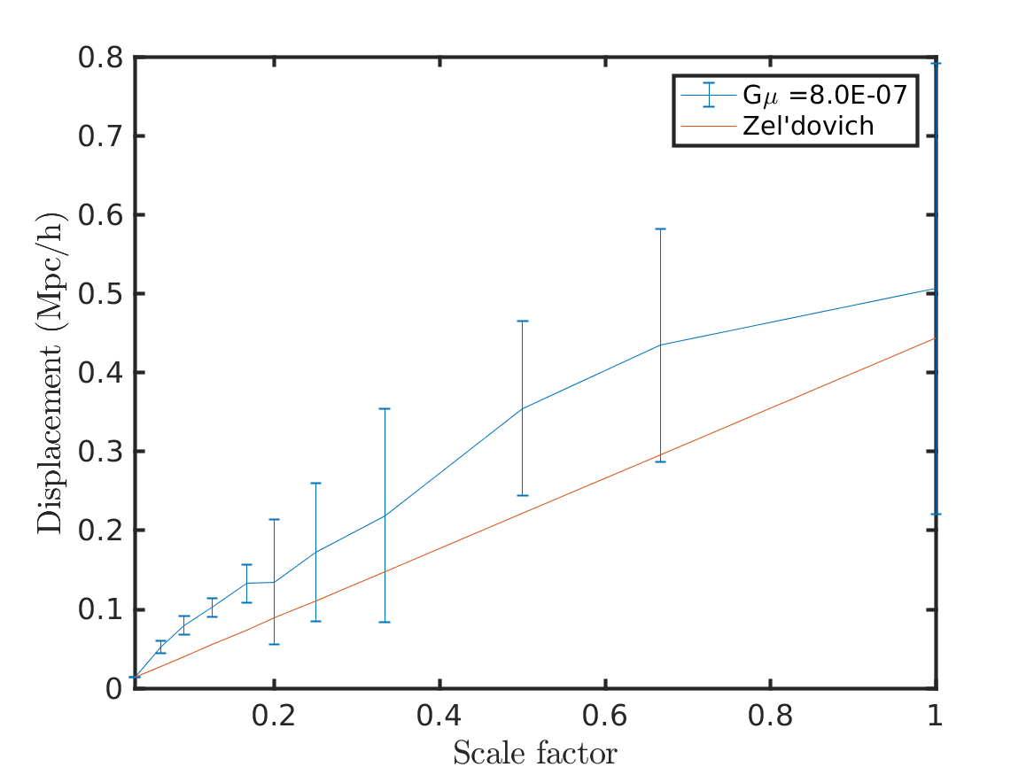
Figure 4: Plot of the displacement induced by the wake (in blue) for different values of the scale factor. The expected displacement evolution from Zel’dovich approximation is shown in red.

It can be seen from the results that the displacement induced by the wake in the simulation grows linearly in the scale factor as it should. However, in the worst case, it is about two times higher than the expected value.

III.4 Simulations

After these checks of the numerical code we will turn to the Guillimin “production” runs. We performed $10$ simulations without wakes. From the $10$ samples, the first three were chosen for wake insertion and evolution, adding to the dataset three samples with $G\mu=10^{-7}$ wakes and three with $G\mu=8\times 10^{-7}$ wakes. The lower value of $G\mu$ was chosen to be just slightly below the current limit on the string tension, the second one is a larger value for which the string effects are manifest and which can be used as a guide for the analysis.

All simulations have a grid of $1024$ cells per dimension and $512$ particles per dimension. The volume of the simulations is $(64)^{3}(h^{-1}{\rm Mpc})^{3}$. The initial conditions were laid down at a redshift of $z=63$, and the wake was inserted at redshift $z=31$. To obtain a better resolution of the wake at the time of wake insertion we also ran simulations where the wake was inserted at redshift $z=15$. A later time of wake insertion, however, then leads to simulations where the effects of the $\Lambda$CDM fluctuations on the wake are neglected for a longer time. We will show that our final results do not depend sensitively on the redshift of wake insertion.

Figure 5 shows output maps of simulations at a range of redshifts. Output map sequences of simulations without a wake, including a wake with $G\mu=8\times 10^{-7}$, and a wake with $G\mu=10^{-7}$ are shown. The wake is placed at the center of the box along the x-axis (the horizontal axis), and is taken to lie in the y-z plane. The y-axis is the vertical axis, and the mass has been projected along the z-direction.

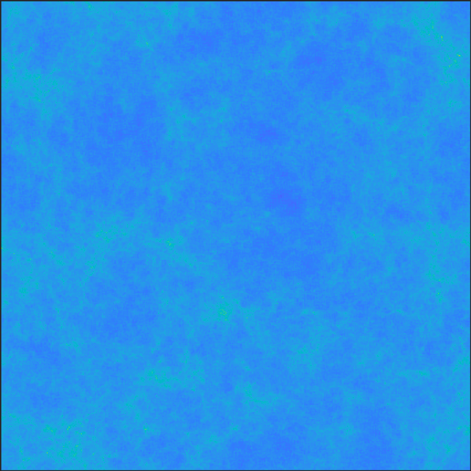
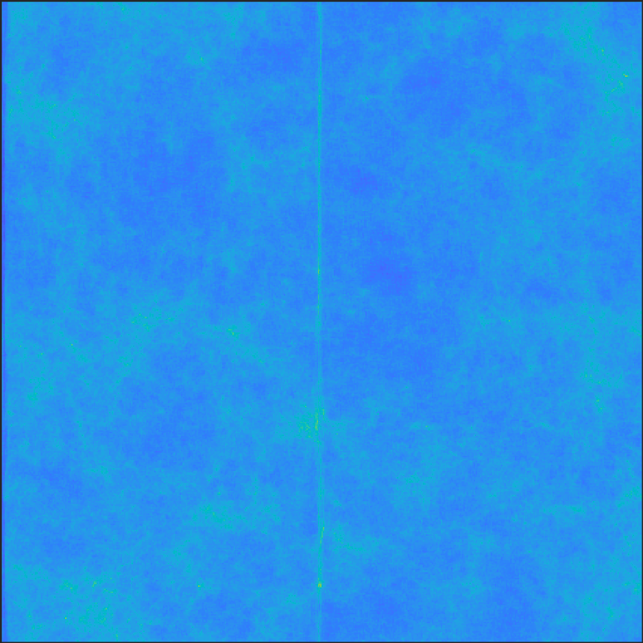
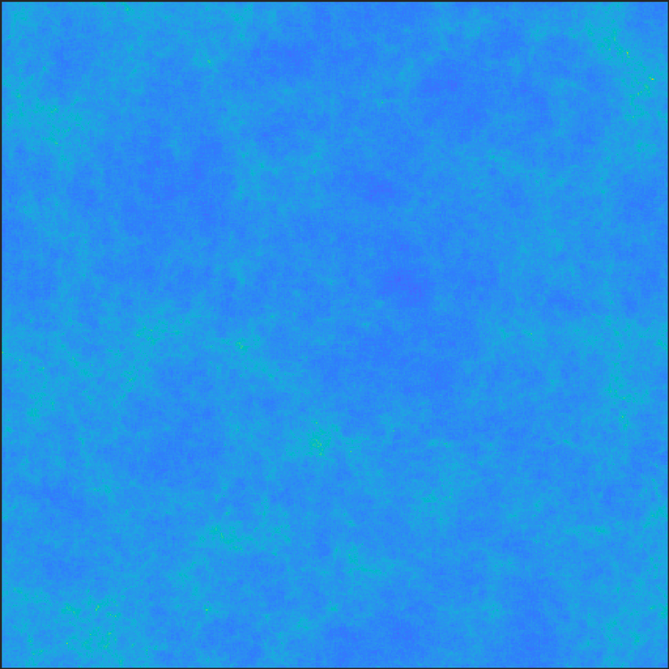
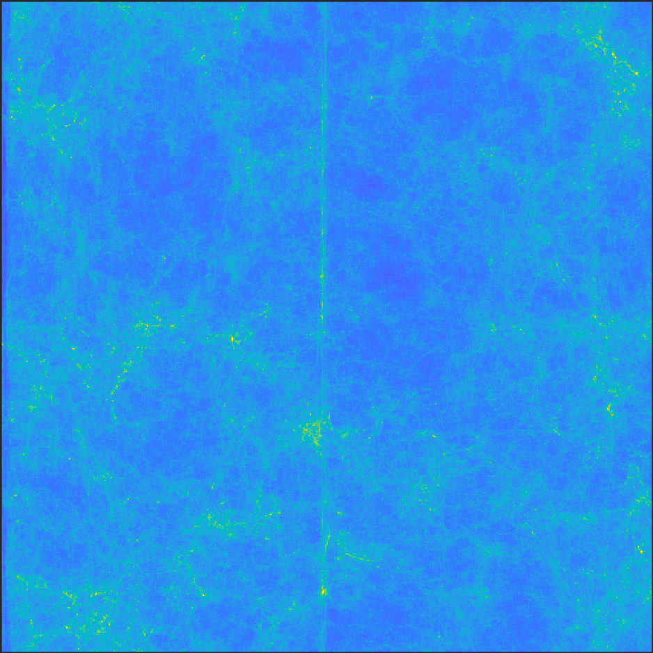
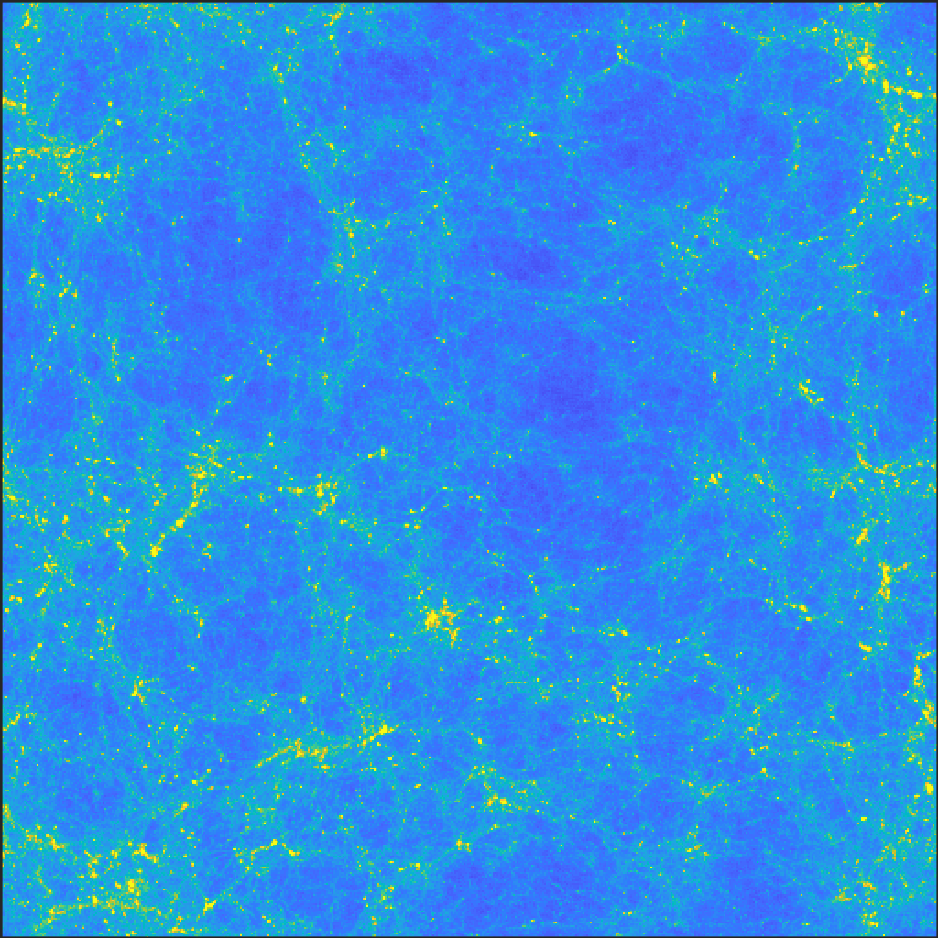
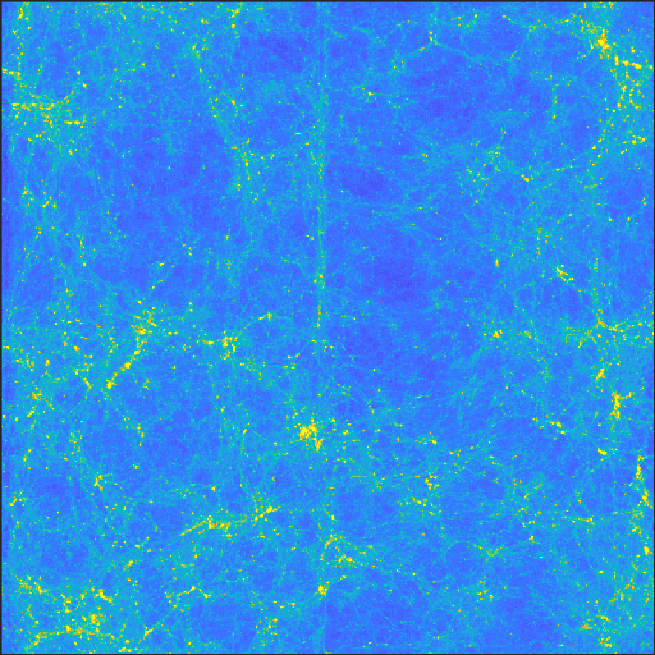
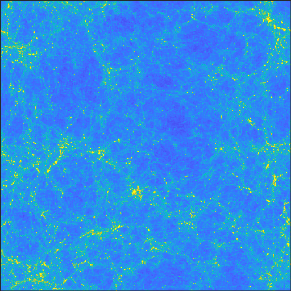
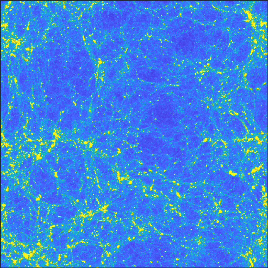
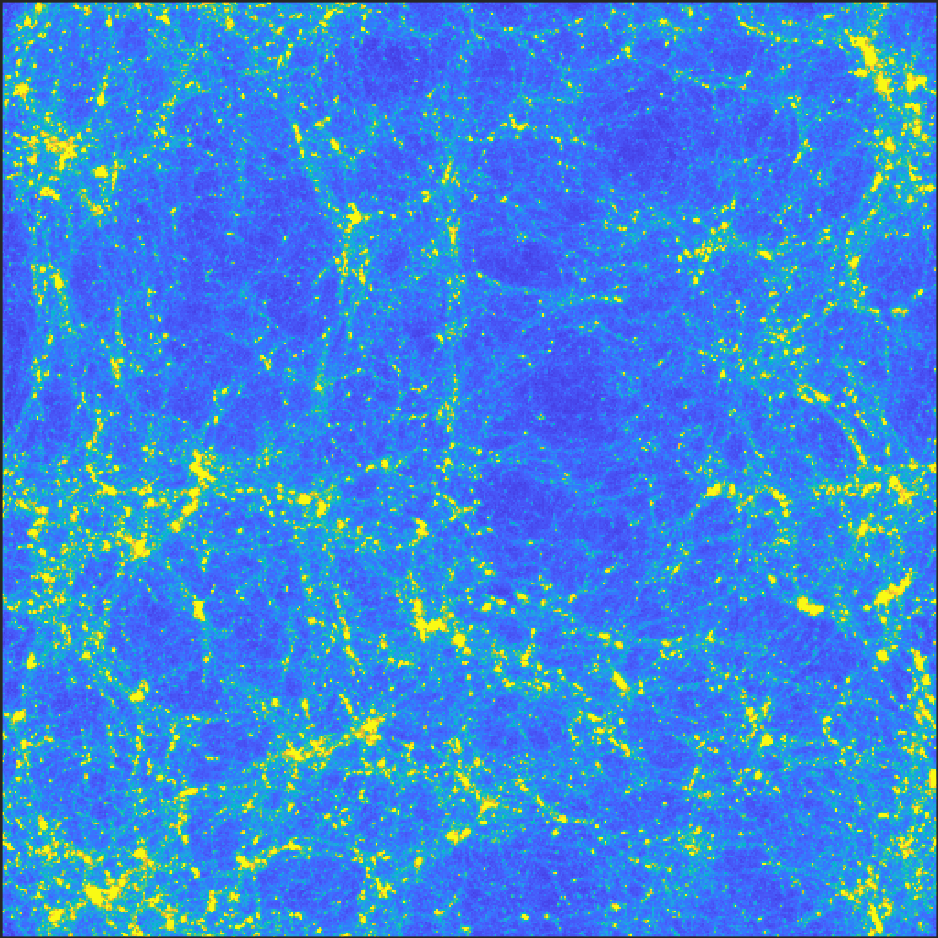
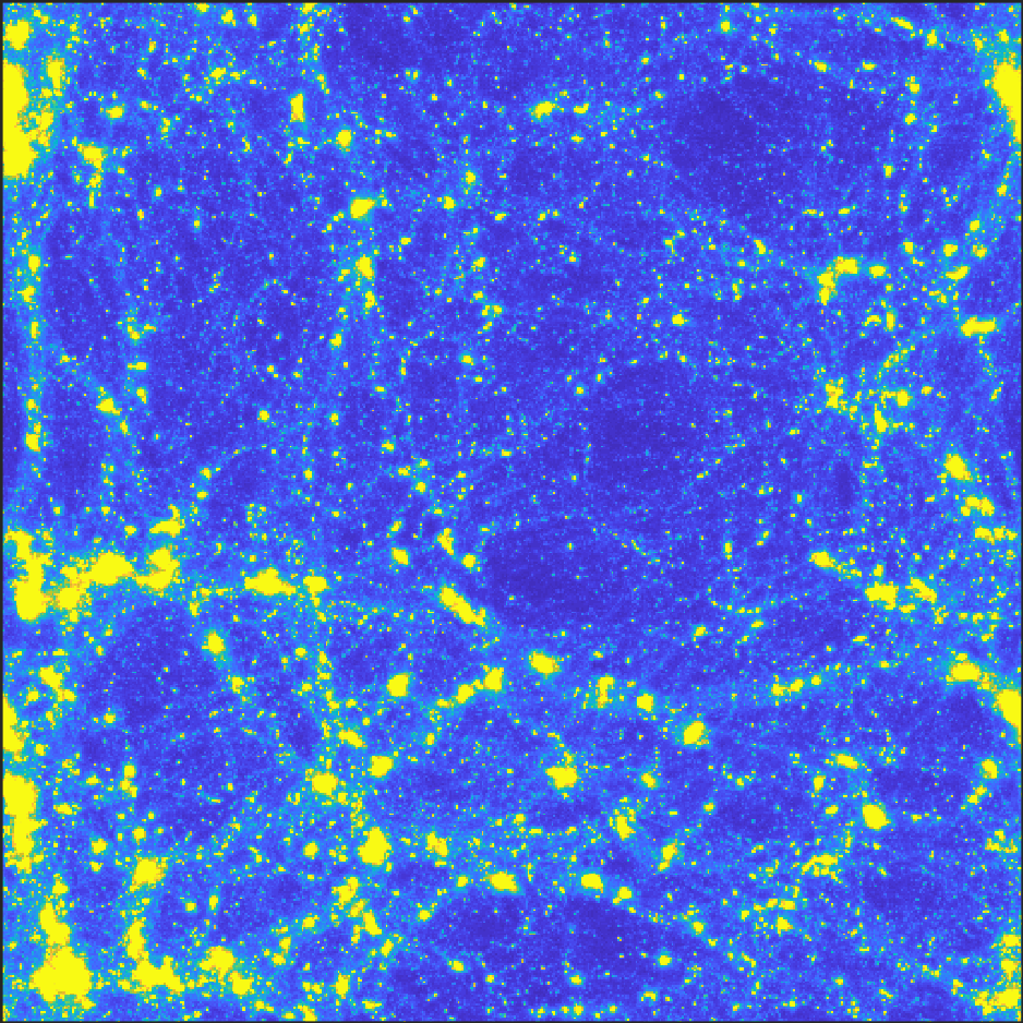
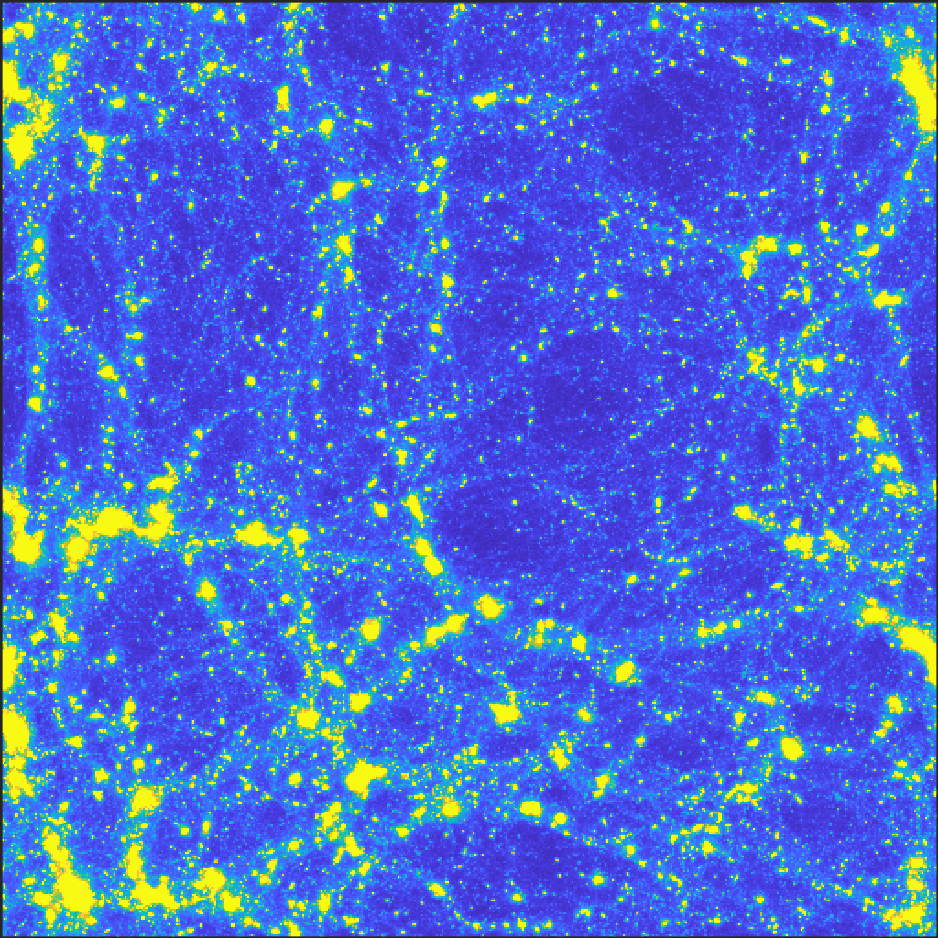
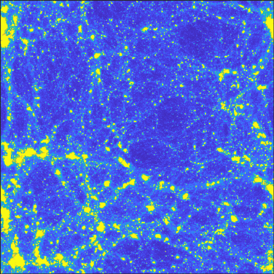
Figure 5: Each panel shows the density contrast of the density field projected in a $(64h^{-1}{\rm Mpc}/h)^{2}$ area. Each row depicts a redshift snapshot, chosen to be $z=10,7,4,2,0$ from top to bottom. The left column corresponds to pure $\Lambda CDM$, the middle contains a $G\mu=8\times 10^{-7}$ wake and the right column contains a $G\mu=1\times 10^{-7}$ wake. The color bar on the bottom associates each color with the corresponding density contrast

Note that the initial thickness of the wake is $5\%$ of the resolution of the simulation. With better resolution the wake would be more clearly visible, in particular at higher redshifts. Given the same computing power, we could increase the local resolution at the cost of reducing the total volume, and we could study the optimal values for the identification of the string signals. This challenge is similar to the challenge on the observational side, where observation resolution and sky coverage need to be balanced.

The leftmost column of Figure 5 shows the resulting mass distribution for redshifts $z=10,7,4,2,0$ in a simulation without a wake, the middle column gives the corresponding output maps for a simulation including a wake with $G\mu=8\times 10^{-7}$, and with the same realization of the Gaussian noise. The wake leads to a planar overdensity of mass which is visible by eye as a linear overdensity along the y-axis. Until redshift $z=4$ the wake is hardly distorted by the Gaussian noise (it appears as an almost straight line in the plots). At redshift $z=2$ the linear overdensity is still clearly visible, although the Gaussian perturbations dominate the features of the map. By redshift $z=0$ the wake has been disrupted, although the remnants of the linear discontinuity are still identifiable. The challenge for a statistical analysis is to extract the wake signal at the lowest redshifts in a quantitative way. The rightmost column of Figure 7 shows the corresponding output maps for a simulation including a wake with $G\mu=10^{-7}$, again with the same realization of the Gaussian noise. In this case, the wake is a factor of $8$ thinner and creates primordial fluctuations which are suppressed by the same factor. The planar overdensity due to the wake is only (and even then only extremely weakly) identifiable at redshift $z=10$. The challenge will be to extract this signal in a manifest way.

IV Statistical Analysis

IV.1 1-d Projections

Our first step in the statistical analysis of the output maps is to consider a further projection of the density, namely a projection onto the direction perpendicular to the wake. Figure 6 shows the resulting distributions for a selection of redshifts (decreasing from top to bottom) for a simulation without a wake (left column), including an added wake with $G\mu=8\times 10^{-7}$ (middle column) and $G\mu=10^{-7}$ (right column), in both cases with the same realization of the Gaussian noise. The vertical axis shows the relative density contrast, the horizontal axis is the coordinate perpendicular to the wake. The wake corresponds to the peak located at distance $d_{z}\simeq 32h^{-1}{\rm Mpc}$ At redshifts $z=15$ and $z=10$ the wake can be clearly identified by eye at this redshift even for $G\mu=10^{-7}$.

As the wake gets disrupted by the Gaussian noise, the wake signal gets harder to identify at lower redshifts. For $G\mu=10^{-7}$ the signal can be seen at redshift $z=10$, but it has disappeared by $z=7$, while for $G\mu=8\times 10^{-7}$ the signal is still present at $z=3$, but no longer at $z=0$.

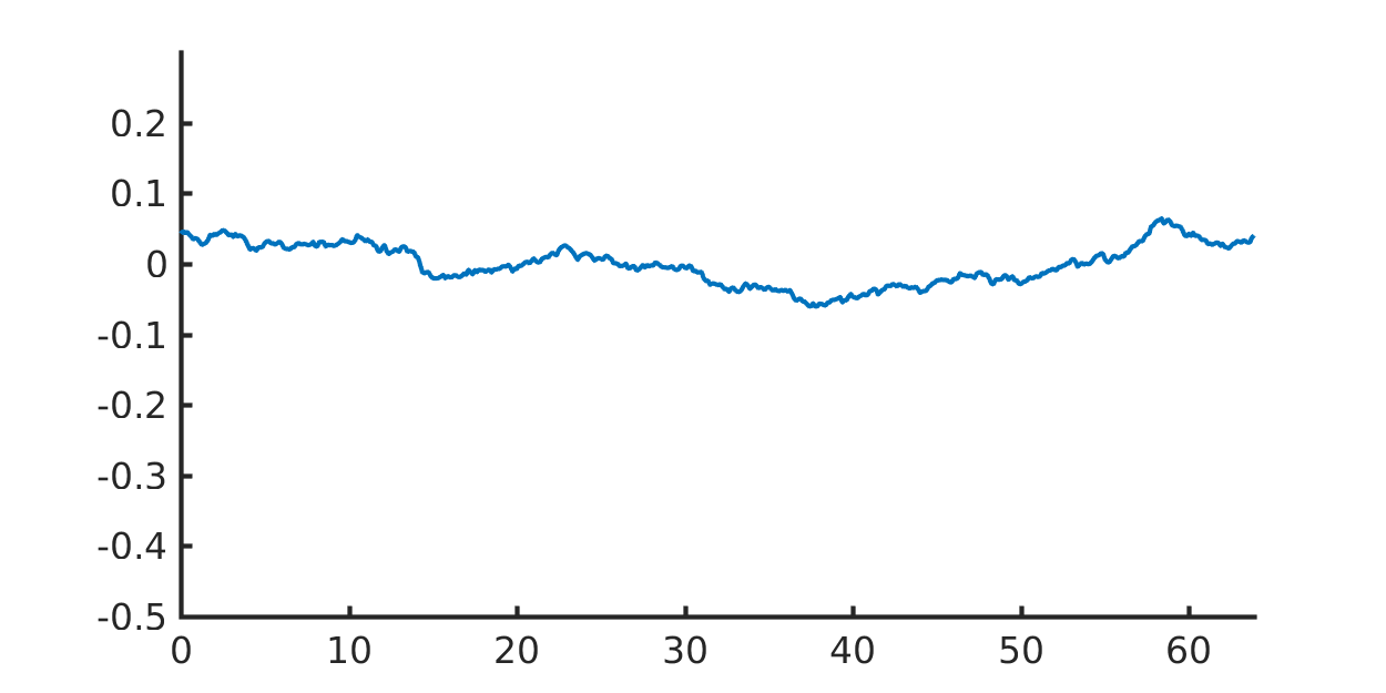
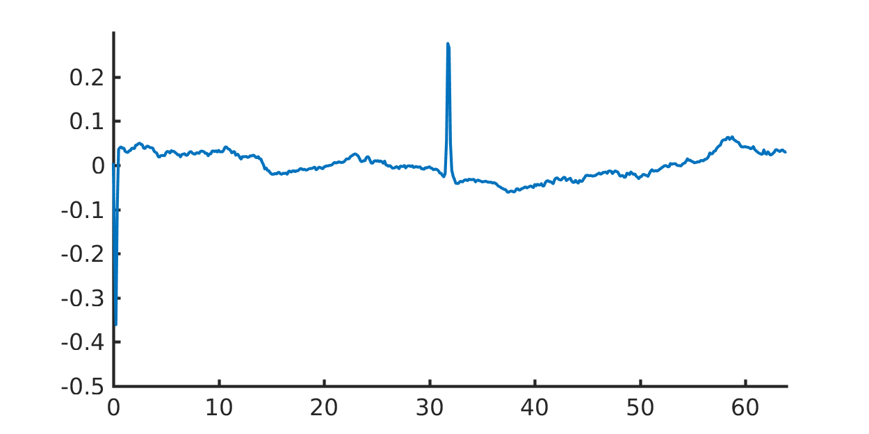
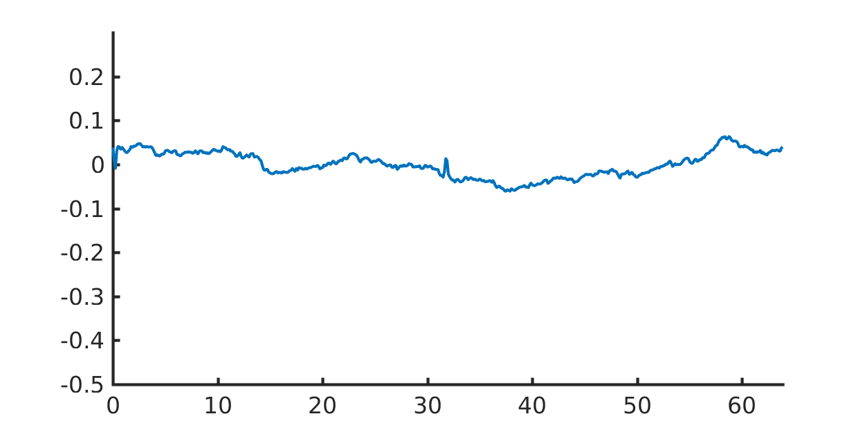
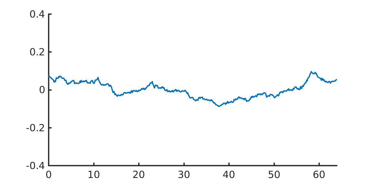
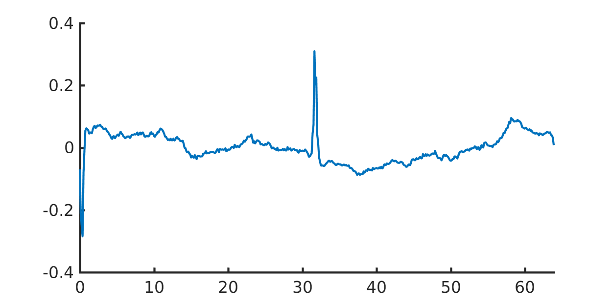
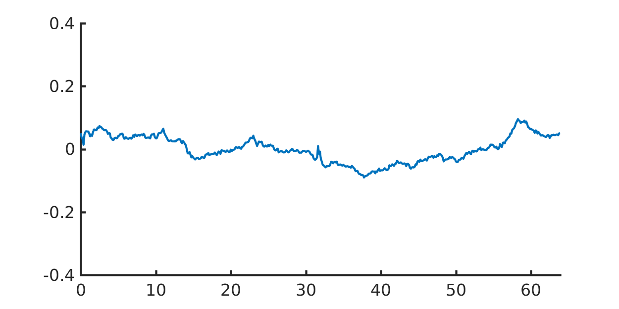
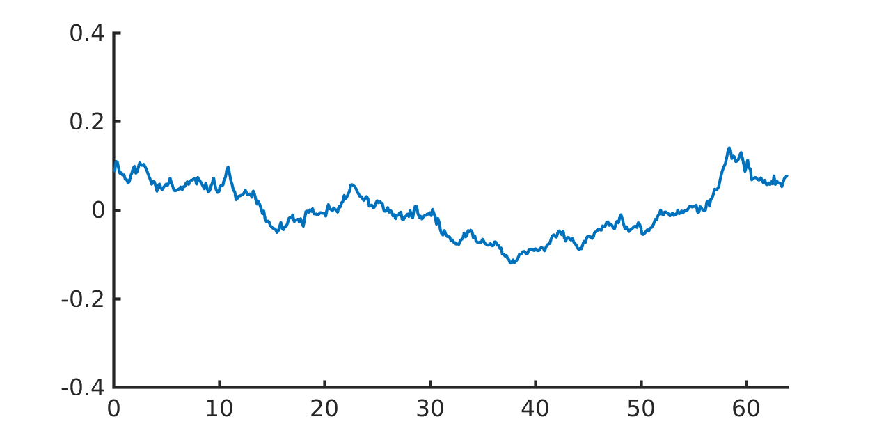
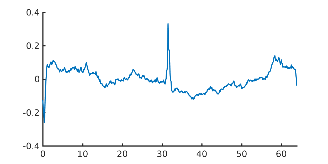
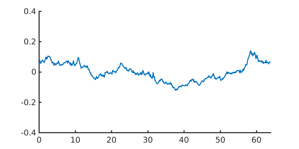
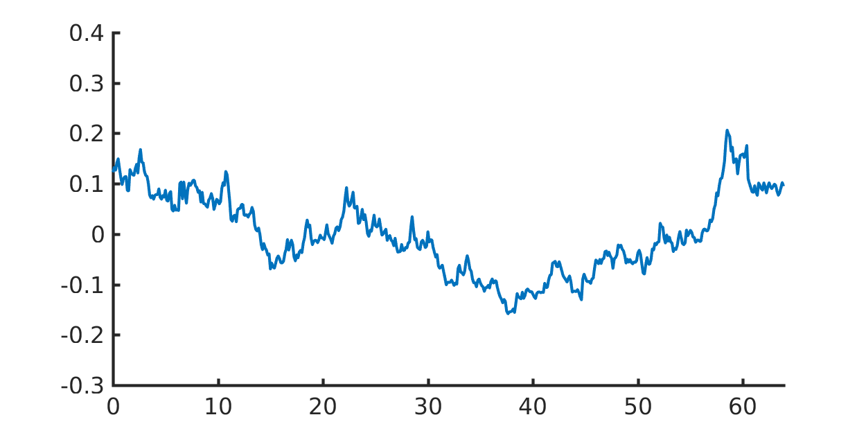
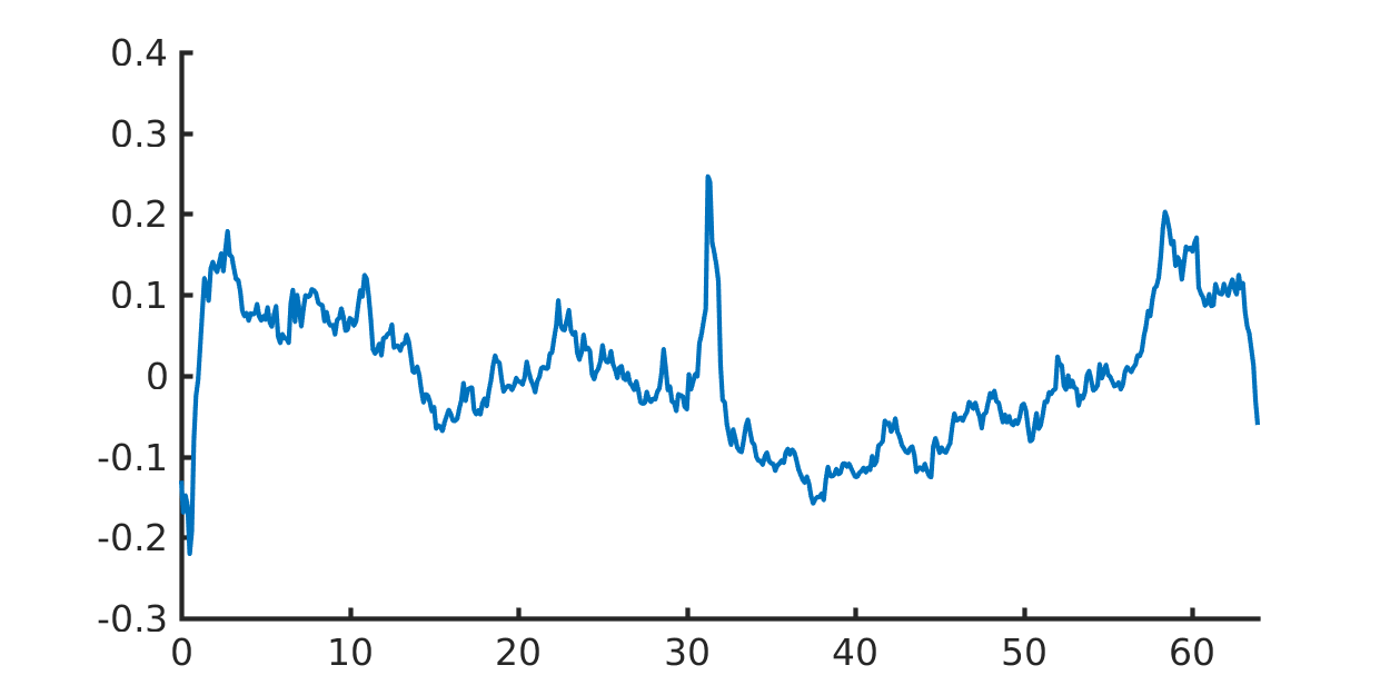
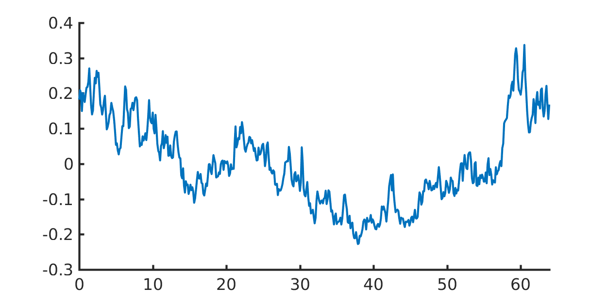
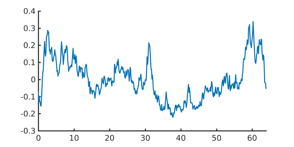
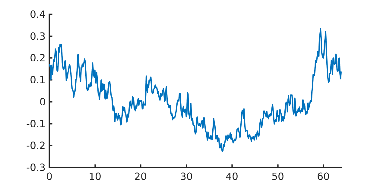
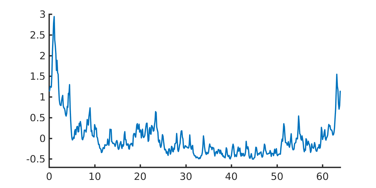
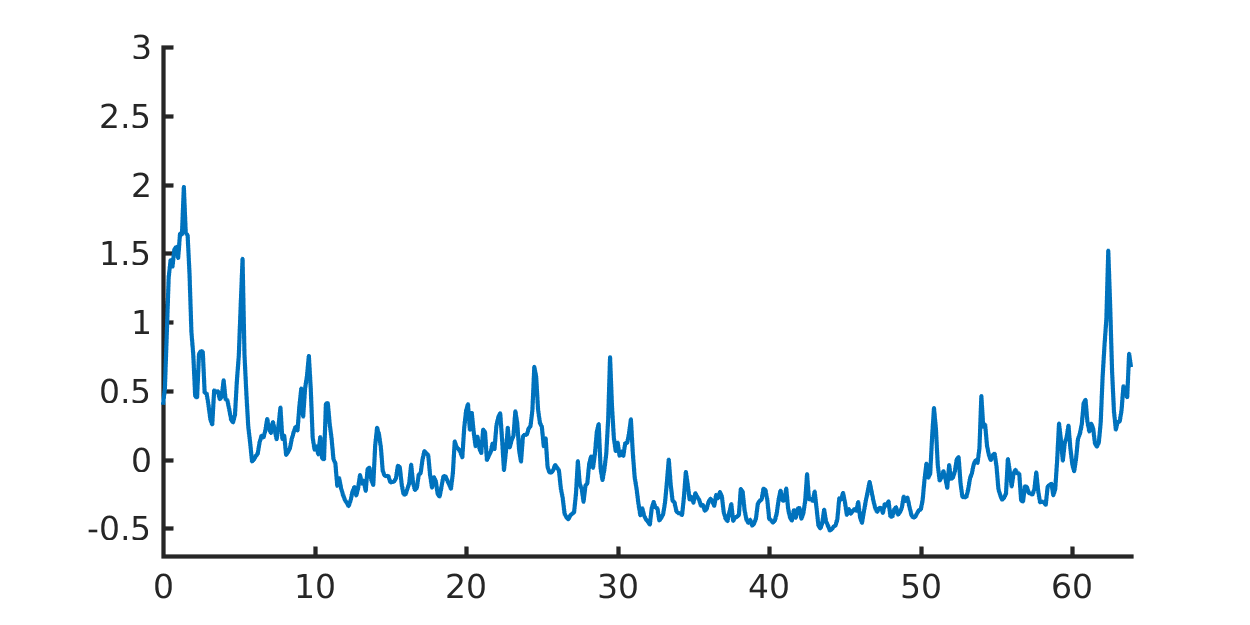
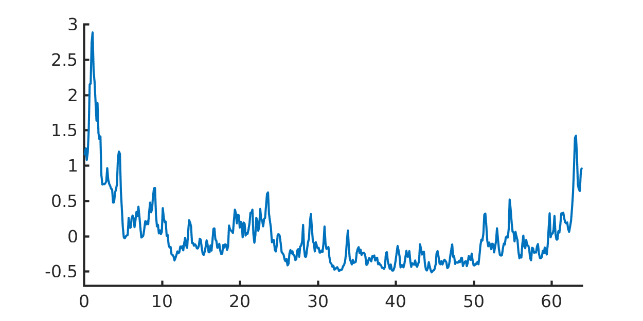
Figure 6: Each panel shows the density contrast of the density field projected in a $(64\ {\rm Mpc}/h)$ axis perpendicular to the wake, when there is one. Each row depict a redshift snapshot, chosen to be $z=15,10,7,5,3,0$ from top to bottom. The left column corresponds to pure $\Lambda CDM$, the middle contains a $G\mu=8\times 10^{-7}$ wake and the right column contains a $G\mu=1\times 10^{-7}$ wake.

Wakes are very thin compared to the scale where the power spectrum of the Gaussian density perturbations peaks. This is particularly true for lower values of the string tension. Hence, a promising method of rendering the wake signal more visible is to perform a wavelet transform of the 1-d projection plots.

We have applied the continuous Morse wavelet transformation Morse to the above 1-d projection plots, and below we show some of the results. The basis used for the continuous wavelet transformation is the Generalized Morse Wavelet Morse which has two parameters: $\beta$, measuring compactness and $\gamma$, characterizing the symmetry of the Morse wavelet. We choose $\gamma=3$ (corresponding to the symmetric case). There are few oscillations if we choose $\beta$ close to $\gamma$, so $\beta=3.01$ is suitable for discontinuities detection. The wavelets are thus characterized by the position $Z$ where they are centered, and by their scale parameter (width) $w$. In the following plots of figure 7), the horizontal axis is $Z$, the vertical axis is the scale parameter. The color is a measure of the modulus of the wavelet coefficients.

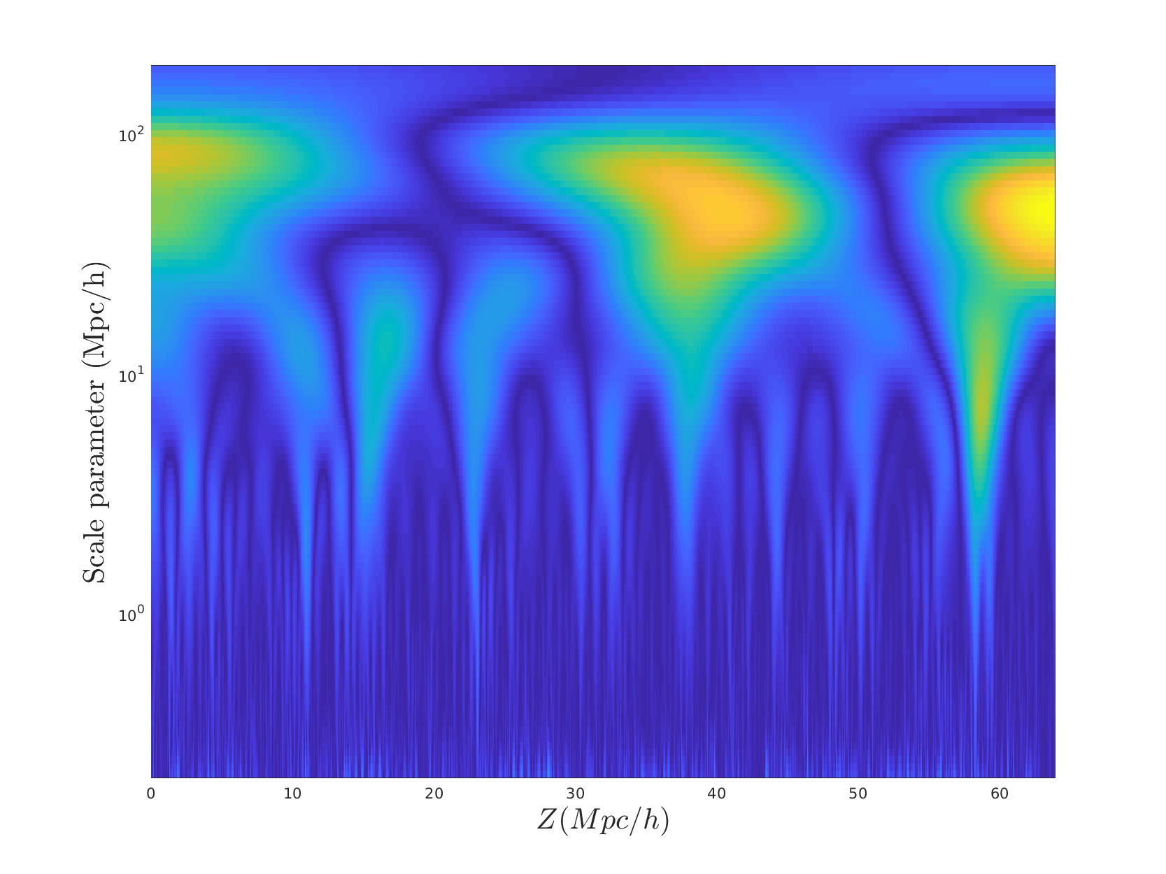
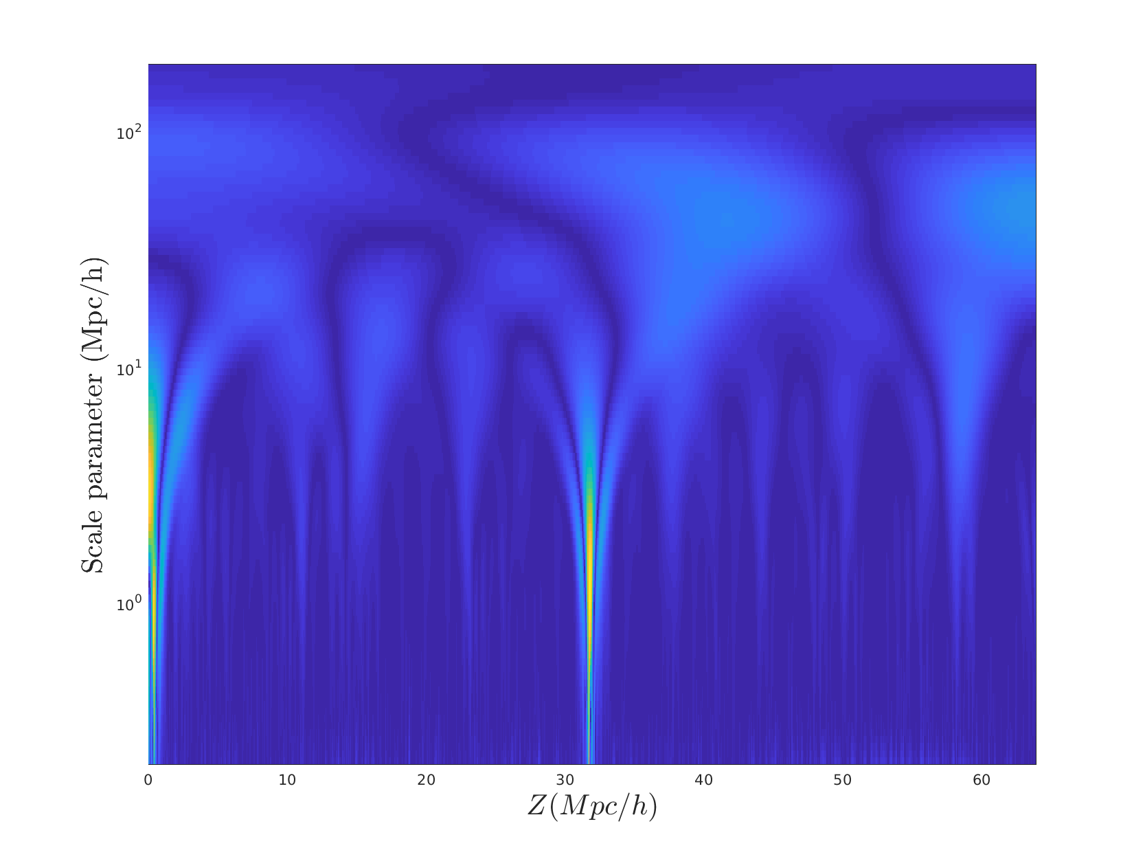
Figure 7: Continuous wavelet transforms of the density contrast of the 1-d projected dark matter density. The horizontal axis is the position parameter of the wavelet decomposition (with $Z=32$ being the position of the wake), and the vertical axis is the width of the wavelet. The top panel is for a simulation without a wake, the middle panel includes a wake with $G\mu=8\times 10^{-7}$, and the bottom panel has a wake with $G\mu=10^{-7}$. Note that the $\Lambda$CDM fluctuations are the same in all three simulations.

A wake is a very thin feature at a particular value of $Z$. Hence, the wave signal will be concentrated at the lowest values of the scale parameter. Figure 9 shows a comparison between the wavelet transformation coefficients in simulations without a wake (top) and including a wake with $G\mu=10^{-7}$ (bottom) and $G\mu=8\times 10^{-7}$ (middle), all at a redshift of $z=10$. The Gaussian noise gives rise to features in the continuous wavelet map which are mostly concentrated at large scale parameters, although there are some features which also appear at small scale parameters. As seen in the bottom panel of Figure 7, the wake adds a narrow feature at the value of $Z$ where the wake is centered which continues to $w\simeq 0.4h^{-1}{\rm Mpc}$. It can be characterized as a narrow spike. The wake-induced spike and the spike-like features in the no-wake simulation can be distinguished in that the features coming from the Gaussian noise weaken as $w$ approaches its minimum value, and are wider than the wake-induced spike. Note that the color scaling is the same in the three panels. We see that the wake signal stands out very strong at $z=10$ for a wake with $G\mu=10^{-7}$, and that it totally dwarfs all other features for $G\mu=8\times 10^{-7}$. The above maps are obtained for a high resolution sampling along the $Z$ direction (we move the center position of the wavelet in steps of $0.5$ of the grid size).

Since the wavelet expansion is an expansion in a complete set of functions, it is possible to reconstruct the original data from the wavelet transform. By setting to zero all wavelet coefficients corresponding to scales higher that a given cutoff, here taken as $0.4h^{-1}{\rm Mpc}$, we can construct filtered 1-d projection graphs in which the long wavelength contributions of the Gaussian noise are eliminated and in which the string wake signal is more clearly visible. If we apply the reconstruction algorithm to the filtered wavelet maps, we can construct a filtered 1-d projection graph in which the long wavelength contributions of the Gaussian noise are eliminated and in which the string wake signal is more clearly visible.

Figure 8 show the reconstructed filtered 1-d projection graphs at redshift $z=10$ in the case of pure Gaussian noise (top panel), and including a string wake with $G\mu=10^{-7}$ (bottom panel) and $G\mu=8\times 10^{-7}$ (middle panel). As in the previous two graphs, the horizontal axis is the coordinate $Z$, and here the vertical axis is the density contrast. The wake signals are greatly enhanced compared to what can be seen in the unfiltered projection graphs. For the value of $G\mu=10^{-7}$, the wake signal is now almost an order of magnitude higher in amplitude than the peak value in the case of pure $\Lambda$CDM fluctuations.

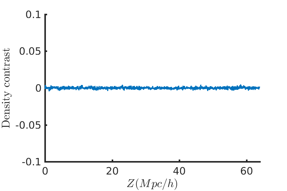
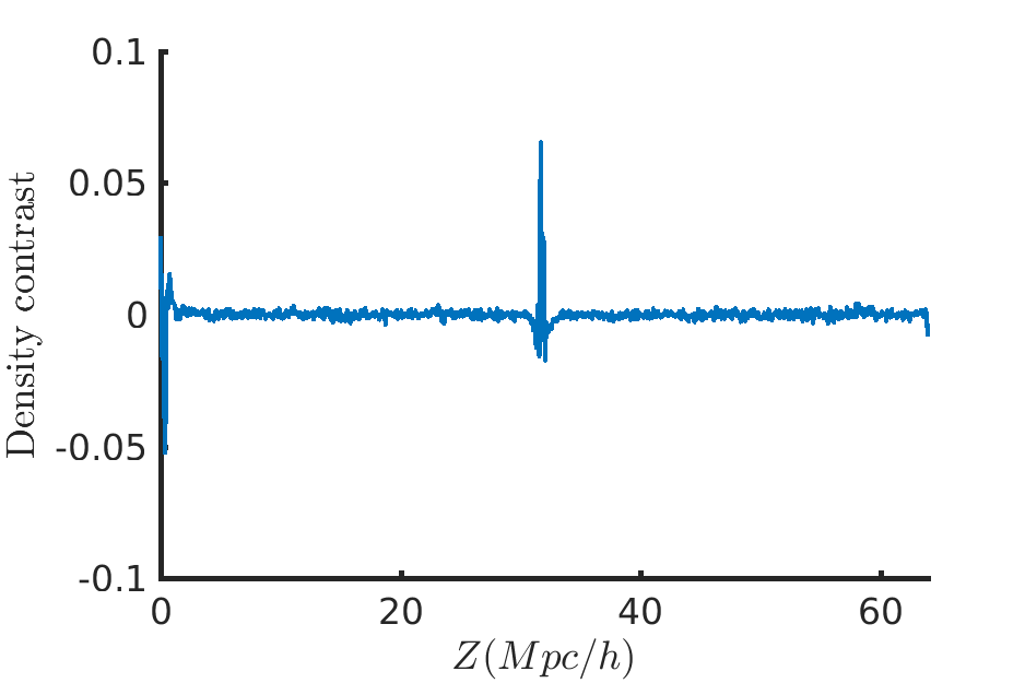
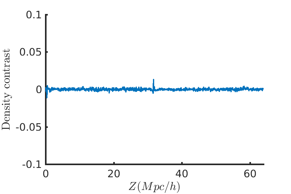
Figure 8: Reconstruction of the 1-d density contrast from the filtered wavelet transforms. The vertical axis is the density contrast, the horizontal axis is the distance of the projection plane from the wake plane. The top panel is the result of a simulation without a wake, the middle panel has a wake with $G\mu=8\times 10^{-7}$, and the bottom panel has a wake with $G\mu=10^{-7}$. The data is for a redshift $z=10$. Note that the wake signal is greatly enhanced compared to the original 1-d projection graphs of Fig. 8.

To show a comparison, we can apply the continuous wavelet transformation to the one-dimensional projection filtered map, obtaining Figure 9. Comparing Figures 9 and 7 we see that the wake signal has been greatly enhanced by filtering.

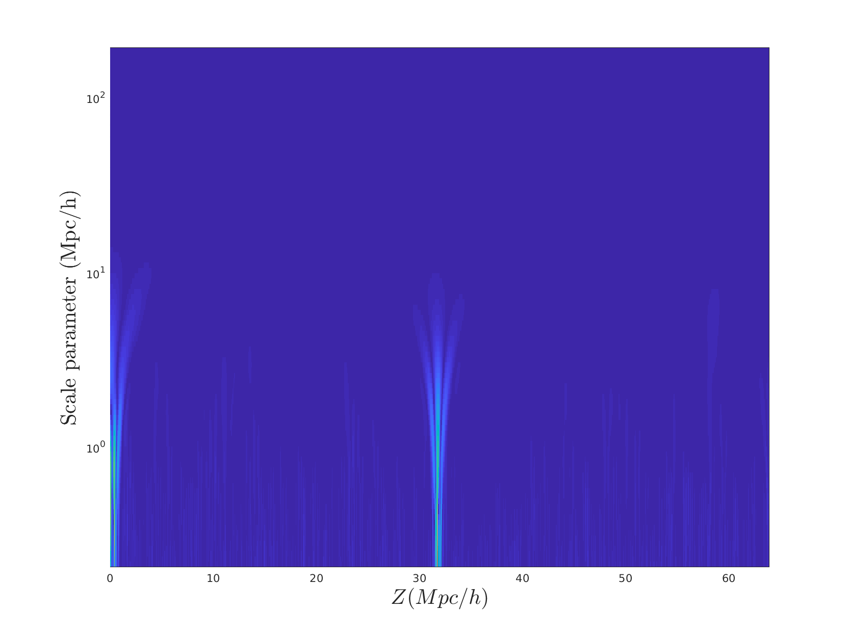
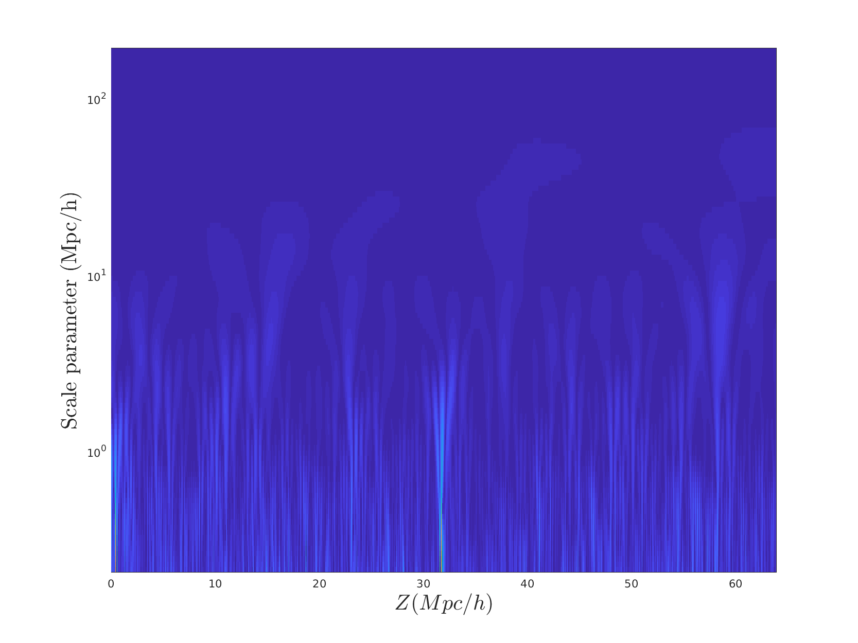
Figure 9: Continuous wavelet transforms after filtering. The axes are like in the figure 7. The top panel is without a wake, the middle panel has a wake with $G\mu=8\times 10^{-7}$, and the bottom panel is for a wake with $G\mu=10^{-7}$.

A statistic which can be used to quantify the significance of the wake signal is the signal to noise ratio ${\cal R}$ which we define to be

$${\cal R}\,=\,\frac{s\ -\bar{n}}{\sigma(n)}\,,$$ (14)

where $s$ is the peak value of the filtered 1-d projection graph with a wake, and $\bar{n}$ is the mean of the peak value of the filtered 1-d projection graph without a wake for the 10 samples and $\sigma(n)$ is the standard deviation of the peak value of the filtered 1-d projection graph without a wake for the same 10 samples.

We find that the average of the signal to noise ratio is

$${\cal\bar{R}}\,=\,17.07\pm 0.83\,,$$ (15)

at redshift $z=10$ in the case of a wake with $G\mu=10^{-7}$ initially laid down at redshift $z=15$ (the error bars are the standard deviation based on three simulations). Hence, we find that a cosmic string wake is identifiable with a $17.07\sigma$ significance. At redshift $z=7$ the difference in the signal to noise is no longer statistically significant.

The results of the signal to noise analysis are given in the following figure (10). The horizontal axis gives the redshift (early times on the left), and the vertical axis is the signal to noise ratio. The bottom curve gives the results for a pure $\Lambda$CDM simulation, the next pair of curves (counting from bottom up) give the results of a simulation where a wake with $G\mu=10^{-7}$ is added, and the top two curves correspond to adding a wake with $G\mu=8\times 10^{-7}$. The two members of the pair correspond to different redshifts of inserting the wake. The difference in the predictions by changing the wake insertion time is not statistically significant.This figure shows the signal to noise ratios of the reconstructed 1-d projection graphs after wavelet transformation and filtering, for the high sampling scale. For $G\mu=10^{-7}$ the wake effect can be clearly seen up to a redshift of $z=10$, and for $G\mu=8\times 10^{-7}$ up to a redshift of $z=5$.

IV.2 Spherical Statistic

In the previous analysis, the statistical analysis was based on an algorithm which presupposed knowing the planar orientation of the wake. For applications to data, we need an analysis tool which does not use this information. In this section we develop such a statistic, which is an adaptation of a 3D ridgelet analysis (Starck ).

The idea is to take the filtered one dimensional projection, similar to Figure 8, for different directions on the sky and compute a relevant quantity. For choosing the angles, a Healpix Gorski:2004by scheme was used with the help of S2LET Leistedt , a free package available at www.s2let.org. The statistic is constructed in the following way: for any direction of the sphere, we consider an associated projection axis passing through the origin of the box. We then consider slices of the simulation box perpendicular to that axis at each point x of it with thickness given by the grid size of the simulation, and we compute the mass density $\delta(x)$ of dark matter particles in that slice as function of x. The range of x is half the simulation box so we avoid slices with small area (compared with the face of the cubic simulation box). A one-dimensional filter wavelet analysis similar to the one described in the previous section is then performed in the mass density $\delta(x)$, giving a filtered version for it, called $f\delta$.

We then compute the maximum value S of $f\delta(x)$ for each direction on the simulation. S is the map on the surface of the sphere which we now consider and $\hat{S}$ is its maximum value. For a simulation including a cosmic string wake with $G\mu=1\times 10^{-7}$ the resulting map at redshift z = 10 is shown in the top left panel of Figure 11, whereas the analysis without the wake is shown in Figure 12. The value of S is indicated in terms of color (see the sidebar for the values).

The wake signal appears at the center of the box and its associated S value is about $40\%$ higher than the maximum of the S value for the map without wake. This can be better visualized in figures 13 and 14, where the center in zoomed in $40$ times. For each map, a peak $\hat{S}$ over standard deviation $\sigma$ of $S$ was computed, and it was found that $\hat{S}/\sigma=8.68$ for a simulation without wake and $\hat{S}/\sigma=14.32$ for the simulation with a $1\times 10^{-7}$ wake.

A wake perpendicular to a particular direction will yield a high signal since the mass in the slice which overlaps with the wake will get a large contribution localized at a particular value of x.

The Healpix scheme does not contain the angles $(\theta,\phi)=(0,0)$ where we know the wake is located, so we never probe the orientation exactly were the wake is. The wake signal has to be reached by increasing the resolution of the analyzed angles. This supports the idea that the information regarding the orientation of the angles should not be included in the analysis.

Figure 10: Signal to noise analysis for the 1-d projections after wavelet transformation, filtering and reconstruction, and for the finer of samplings in wavelet width. The horizontal axis shows the redshift, the vertical axis is the signal to noise ratio. The two pair of curves in the bottom contain an wake with $G\mu=10^{-7}$, and the top two curves are for an wake with $G\mu=8\times 10^{-7}$. The two members of a pair of curves correspond to different redshifts of wake insertion (as is obvious from the starting points of the curves). The points that are not shown correspond to values for the signal to noise equal to zero.

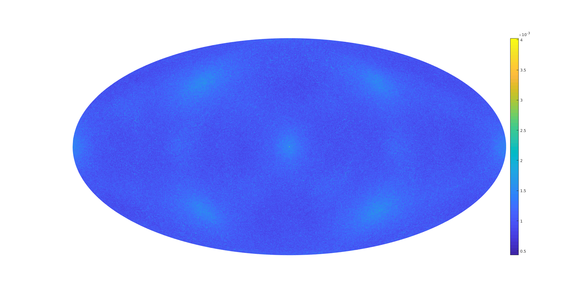
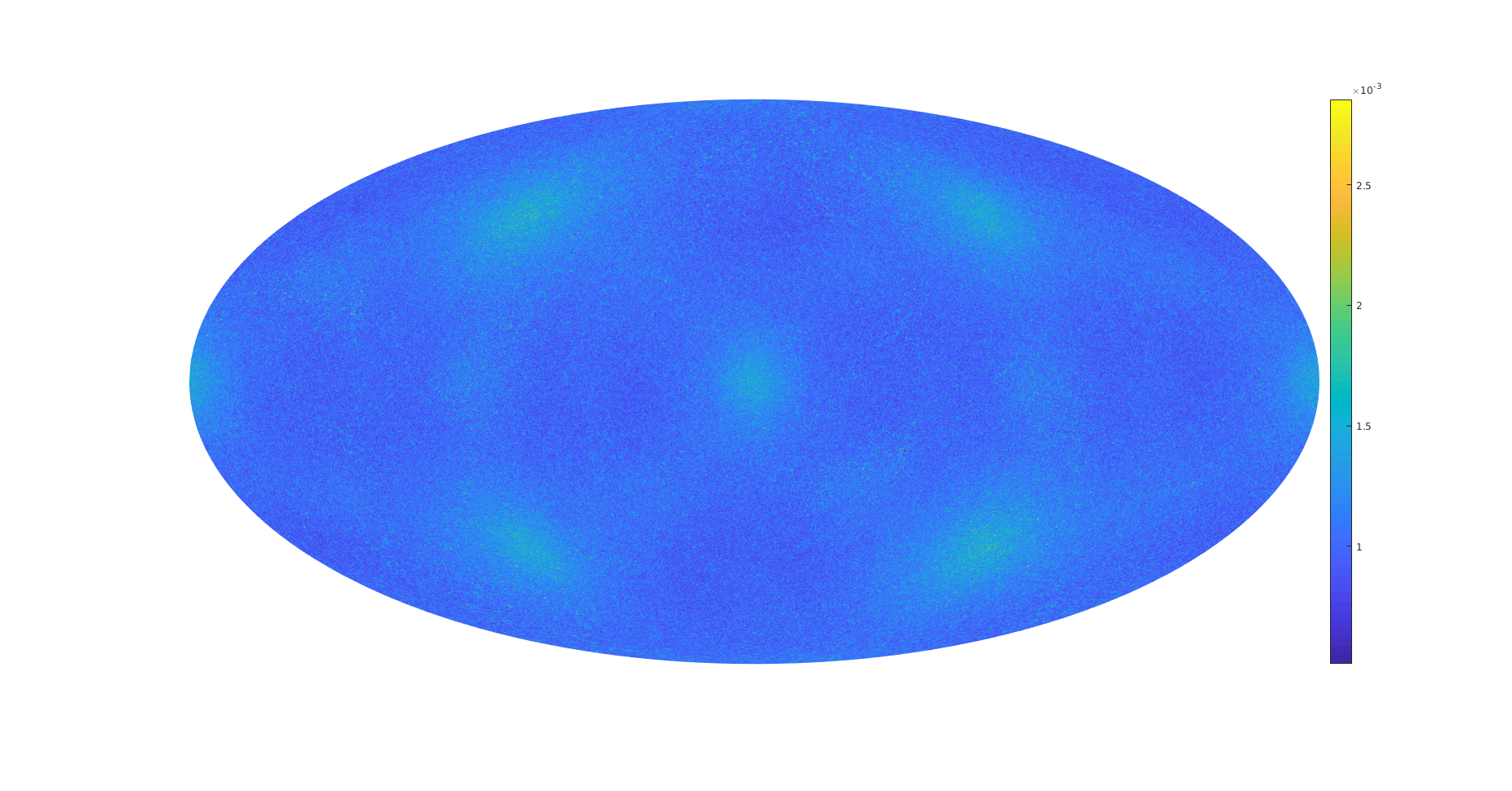
Figure 11: Reconstructed map for a simulation with wake tension $G\mu=1\times 10^{-7}$ at redshift $z=10$.

Figure 12: The same map for a simulation without a wake, at redshift $z=10$.

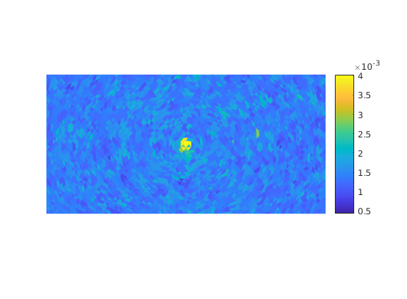
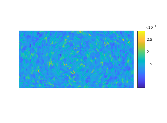
Figure 13: $40\ \times$ zoom of the reconstructed map for a simulation with wake tension $G\mu=1\times 10^{-7}$ at redshift $z=10$.

Figure 14: $40\ \times$ zoom of the the same map for a simulation without a wake, at redshift $z=10$.

At the present level, our analysis shows that cosmic string wakes with a tension of $1\times G\mu=10^{-7}$ can be extracted at redshift $z=10$, as was found in our previous study where knowledge of the orientation of the wake was assumed. In work in progress we are investigating whether string wakes are in fact visible at lower redshifts using this more sophisticated statistic. One could first imagine that an analysis which uses the knowledge of the wake orientation will yield better results than one which does not, but this may not be the case here since the analysis of this section uses more properties which differentiate $\Lambda$CDM fluctuations and wake signals than the previous analysis did.

V Conclusions and Discussion

We have presented the results from N-body simulations of the effects of a planar cosmic string wake on the distribution of dark matter. We have demonstrated that cosmic string signals can be extracted from the background of $\Lambda$CDM fluctuations by considering the three dimensional distribution of dark matter. Given the current resolution of the simulations, a threshold of

$$G\mu\,=\,10^{-7}$$ (16)

can be reached if the dark matter distribution is considered at redshift $z=10$. This value of the string tension is competitive with the current limit which stems from the angular power spectrum of CMB anisotropies. With improved resolution, improved limits may be within reach. This means that the string signal might be identifiable for $G\mu=10^{-7}$ even at redshifts lower than $z=10$, and for smaller values of $G\mu$ at redshift $z=10$.

Key to this work is that we are looking for the specific non-Gaussian signals which cosmic string wakes induce in position space. Position space algorithms are much more powerful at identifying cosmic string signals than by focusing simply on the power spectrum. It is possible that with improved statistical tools, better limits on the string tension can be reached. Work on this question is in progress.

Searching for signals of individual cosmic string wakes in position space has a further advantage compared to studying only the power spectrum: the position space algorithms are to first approximation insensitive to the number $N$ of strings passing through each Hubble volume. This number is known only to within an order of magnitude, although we know from analytical arguments (see e.g. RHBCSrev ) that $N$ should be of the order one. In particular, this means that the constraint (2) on $G\mu$ from the angular power spectrum of CMB anisotropies is sensitive to the value of $N$ which is assumed, whereas our analysis is not.

In this work we have shown that by analyzing the distribution of dark matter, an interesting threshold value of the cosmic string tension can be reached. In future work, we plan to explore how changing the size of the simulation box, the spatial resolution of the simulations, and the sampling width can lead to improved bounds.

So far we have considered simulations with a single cosmic string wake. An extension of our work will involve studying the effects of a full scaling distribution of strings. This work will be conceptually straightforward but computationally intensive. Another extension for the current work would be to consider curvelet-like signal extraction, in which segments of the wake would be detected, possibly giving more information about the wake presence when it is bended due the the $\Lambda CDM$ fluctuations at low redshifts and it is not a plane anymore.

In order to compare our simulation results to observational surveys, we need to extend our work in several ways. To compare our work with optical and infrared galaxy survey results, we need to identify halos from our distribution of dark matter, and run the statistical tools on the resulting distribution of halos. The N-body code we are using already contains a halo-finding routine. Hence, this extension of our work will also be straightforward.

As we have seen, the string signals are much easier to identify at higher redshifts. Hence, 21cm surveys might lead to tighter constraints on the cosmic string tension. At redshifts lower than the redshift of reionization, most of the neutral hydrogen which gives 21cm signals is in the galaxies. Hence, the distribution of 21cm radiation could be modeled by considering the distribution of galaxy halos obtained from our simulations and by inserting into each halo the distribution of neutral hydrogen obtained recently in the study of Hamsa . We plan to tackle this question in the near future.

The effect of cosmic strings on the 21cm signal from the Epoch of Reionization is a more difficult question. Here, the ionizing radiation from cosmic string loops (e.g. via cosmic string loop cusp decay cusp ) will most likely play a dominant role. Finally, at redshifts greater than that of reionization, string wakes lead to a beautiful signal in 21cm maps: thin wedges in redshift direction extended in angular directions to the comoving horizon at $t_{eq}$ where there is pronounced absorption of 21cm radiation due to the neutral hydrogen in the wake Holder2 .

Appendix A Peak Heights

In this appendix we add a figure showing the distribution of peak heights used in the statistic in Section IV.A. The horizontal axis gives the redshift, the vertical axis is the peak height. Shown are the results for ten simulations without a wake (marked “o”) and for three simulations each with a wake with tension $G\mu=10^{-7}$ inserted at redshift $z=31$ (marked “*”), with the same tension and insertion redshift $z=15$ (marked “+”), with tension $G\mu=8\times 10^{-7}$ and insertion redshifts $z=31$ (marked with inverted triangles) and $z=15$ (marked “x”).

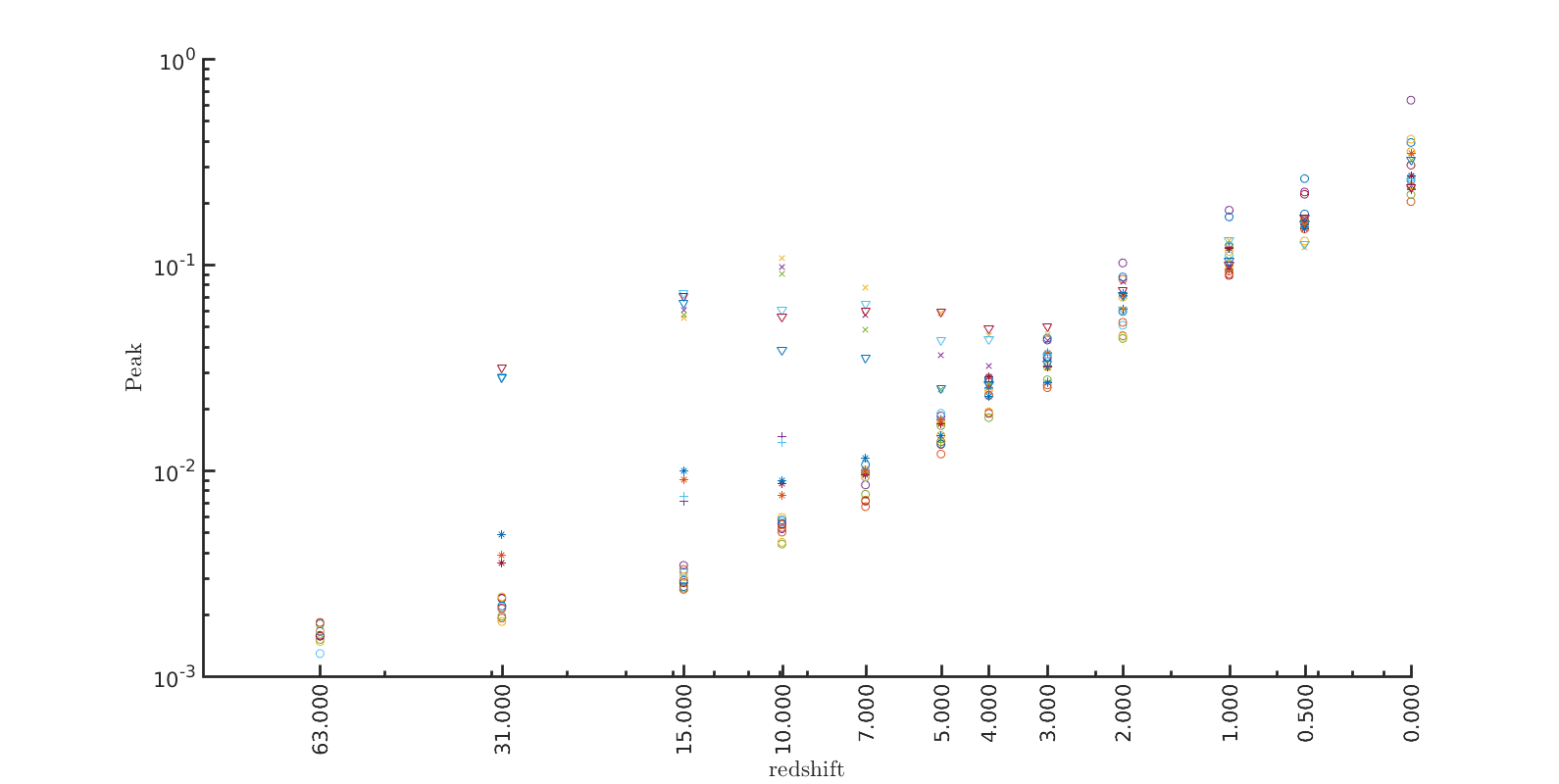
Figure 15: The peak values for simulations without a wake are marked by circles, for those with a wake with tension $Gμ=10^{−7}$ inserted at redshift $z=31$ and $z=15$ by “*” and “+”, respectively, and for those with tension $Gμ=8\times 10^{−7}$ inserted at redshifts $z=31$ and $z=15$ by inverted triangles and “x”, respectively.

From this figure it is clear that wakes with $G\mu=10^{-7}$ are identifiable until redshift of $z=10$ while those with $G\mu=8\times 10^{-7}$ can be identified down to below $z=7$.

References

-
(1)
T. W. B. Kibble,
“Phase Transitions In The Early Universe”,
Acta Phys. Polon. B 13, 723 (1982);
T. W. B. Kibble, “Some Implications Of A Cosmological Phase Transition”, Phys. Rept. 67, 183 (1980). - (2) E. Witten, “Superconducting Strings,” Nucl. Phys. B 249, 557 (1985). doi:10.1016/0550-3213(85)90022-7
- (3) A. Vilenkin and E.P.S. Shellard, Cosmic Strings and other Topological Defects (Cambridge Univ. Press, Cambridge, 1994).
- (4) M. B. Hindmarsh and T. W. B. Kibble, “Cosmic strings”, Rept. Prog. Phys. 58, 477 (1995) [arXiv:hep-ph/9411342].
- (5) R. H. Brandenberger, “Topological defects and structure formation”, Int. J. Mod. Phys. A 9, 2117 (1994) [arXiv:astro-ph/9310041].
-
(6)
A. Albrecht and N. Turok,
“Evolution Of Cosmic Strings”,
Phys. Rev. Lett. 54, 1868 (1985);
D. P. Bennett and F. R. Bouchet, “Evidence For A Scaling Solution In Cosmic String Evolution”, Phys. Rev. Lett. 60, 257 (1988);
B. Allen and E. P. S. Shellard, “Cosmic String Evolution: A Numerical Simulation”, Phys. Rev. Lett. 64, 119 (1990);
C. Ringeval, M. Sakellariadou and F. Bouchet, “Cosmological evolution of cosmic string loops”, JCAP 0702, 023 (2007) [arXiv:astro-ph/0511646];
V. Vanchurin, K. D. Olum and A. Vilenkin, “Scaling of cosmic string loops”, Phys. Rev. D 74, 063527 (2006) [arXiv:gr-qc/0511159];
L. Lorenz, C. Ringeval and M. Sakellariadou, “Cosmic string loop distribution on all length scales and at any redshift”, JCAP 1010, 003 (2010) [arXiv:1006.0931 [astro-ph.CO]];
J. J. Blanco-Pillado, K. D. Olum and B. Shlaer, “Large parallel cosmic string simulations: New results on loop production”, Phys. Rev. D 83, 083514 (2011) [arXiv:1101.5173 [astro-ph.CO]];
J. J. Blanco-Pillado, K. D. Olum and B. Shlaer, “The number of cosmic string loops”, Phys. Rev. D 89, no. 2, 023512 (2014) [arXiv:1309.6637 [astro-ph.CO]]. -
(7)
T. Charnock, A. Avgoustidis, E. J. Copeland and A. Moss,
“CMB Constraints on Cosmic Strings and Superstrings”,
arXiv:1603.01275 [astro-ph.CO];
C. Dvorkin, M. Wyman and W. Hu, “Cosmic String constraints from WMAP and the South Pole Telescope”, Phys. Rev. D 84, 123519 (2011) [arXiv:1109.4947 [astro-ph.CO]]. - (8) P. A. R. Ade et al. [Planck Collaboration], “Planck 2013 results. XXV. Searches for cosmic strings and other topological defects”, Astron. Astrophys. 571, A25 (2014) [arXiv:1303.5085 [astro-ph.CO]].
-
(9)
L. Pogosian, S. H. H. Tye, I. Wasserman and M. Wyman,
“Observational constraints on cosmic string production during brane
inflation”,
Phys. Rev. D 68, 023506 (2003)
[Erratum-ibid. D 73, 089904 (2006)]
[arXiv:hep-th/0304188];
M. Wyman, L. Pogosian and I. Wasserman, “Bounds on cosmic strings from WMAP and SDSS”, Phys. Rev. D 72, 023513 (2005) [Erratum-ibid. D 73, 089905 (2006)] [arXiv:astro-ph/0503364];
A. A. Fraisse, “Limits on Defects Formation and Hybrid Inflationary Models with Three-Year WMAP Observations”, JCAP 0703, 008 (2007) [arXiv:astro-ph/0603589];
U. Seljak, A. Slosar and P. McDonald, “Cosmological parameters from combining the Lyman-alpha forest with CMB, galaxy clustering and SN constraints”, JCAP 0610, 014 (2006) [arXiv:astro-ph/0604335];
R. A. Battye, B. Garbrecht and A. Moss, “Constraints on supersymmetric models of hybrid inflation”, JCAP 0609, 007 (2006) [arXiv:astro-ph/0607339];
R. A. Battye, B. Garbrecht, A. Moss and H. Stoica, “Constraints on Brane Inflation and Cosmic Strings”, JCAP 0801, 020 (2008) [arXiv:0710.1541 [astro-ph]];
N. Bevis, M. Hindmarsh, M. Kunz and J. Urrestilla, “CMB power spectrum contribution from cosmic strings using field-evolution simulations of the Abelian Higgs model”, Phys. Rev. D 75, 065015 (2007) [arXiv:astro-ph/0605018];
N. Bevis, M. Hindmarsh, M. Kunz and J. Urrestilla, “Fitting CMB data with cosmic strings and inflation”, Phys. Rev. Lett. 100, 021301 (2008) [astro-ph/0702223 [ASTRO-PH]];
R. Battye and A. Moss, “Updated constraints on the cosmic string tension”, Phys. Rev. D 82, 023521 (2010) [arXiv:1005.0479 [astro-ph.CO]]. - (10) R. H. Brandenberger, “Probing Particle Physics from Top Down with Cosmic Strings”, Universe 1, no. 4, 6 (2013) [arXiv:1401.4619 [astro-ph.CO]].
- (11) A. Vilenkin, “Gravitational Field of Vacuum Domain Walls and Strings”, Phys. Rev. D 23, 852 (1981).
- (12) J. C. R. Magueijo, “Inborn metric of cosmic strings”, Phys. Rev. D 46, 1368 (1992). doi:10.1103/PhysRevD.46.1368
- (13) N. Kaiser and A. Stebbins, “Microwave Anisotropy Due To Cosmic Strings”, Nature 310, 391 (1984).
-
(14)
J. Silk and A. Vilenkin,
“Cosmic Strings And Galaxy Formation”,
Phys. Rev. Lett. 53, 1700 (1984);
M. J. Rees, “Baryon concentrations in string wakes at : implications for galaxy formation and large-scale structure”, Mon. Not. Roy. Astron. Soc. 222, 27 (1986);
T. Vachaspati, “Cosmic Strings and the Large-Scale Structure of the Universe”, Phys. Rev. Lett. 57, 1655 (1986);
A. Stebbins, S. Veeraraghavan, R. H. Brandenberger, J. Silk and N. Turok, “Cosmic String Wakes”, Astrophys. J. 322, 1 (1987). -
(15)
R. H. Brandenberger, L. Perivolaropoulos and A. Stebbins,
“Cosmic Strings, Hot Dark Matter And The Large Scale Structure Of The Universe,”
Int. J. Mod. Phys. A 5, 1633 (1990);
L. Perivolaropoulos, R. H. Brandenberger and A. Stebbins, “Dissipationless Clustering Of Neutrinos In Cosmic String Induced Wakes,” Phys. Rev. D 41, 1764 (1990). - (16) Y. .B. Zeldovich, “Gravitational instability: An Approximate theory for large density perturbations,” Astron. Astrophys. 5, 84 (1970).
-
(17)
J. Magueijo, A. Albrecht, D. Coulson and P. Ferreira,
“Doppler peaks from active perturbations”,
Phys. Rev. Lett. 76, 2617 (1996)
[arXiv:astro-ph/9511042];
U. L. Pen, U. Seljak and N. Turok, “Power spectra in global defect theories of cosmic structure formation”, Phys. Rev. Lett. 79, 1611 (1997) [arXiv:astro-ph/9704165];
L. Perivolaropoulos, “Spectral Analysis Of Microwave Background Perturbations Induced By Cosmic Strings”, Astrophys. J. 451, 429 (1995) [arXiv:astro-ph/9402024]. -
(18)
R. J. Danos and R. H. Brandenberger,
“Canny Algorithm, Cosmic Strings and the Cosmic Microwave Background”,
Int. J. Mod. Phys. D 19, 183 (2010)
[arXiv:0811.2004 [astro-ph]];
S. Amsel, J. Berger and R. H. Brandenberger, “Detecting Cosmic Strings in the CMB with the Canny Algorithm”, JCAP 0804, 015 (2008) [arXiv:0709.0982 [astro-ph]];
A. Stewart and R. Brandenberger, “Edge Detection, Cosmic Strings and the South Pole Telescope”, JCAP 0902, 009 (2009) [arXiv:0809.0865 [astro-ph]]. - (19) L. Hergt, A. Amara, R. Brandenberger, T. Kacprzak and A. Refregier, “Searching for Cosmic Strings in CMB Anisotropy Maps using Wavelets and Curvelets,” arXiv:1608.00004 [astro-ph.CO].
- (20) J. D. McEwen, S. M. Feeney, H. V. Peiris, Y. Wiaux, C. Ringeval and F. R. Bouchet, “Wavelet-Bayesian inference of cosmic strings embedded in the cosmic microwave background,” arXiv:1611.10347 [astro-ph.IM].
-
(21)
R. Ciuca and O. F. Hernández,
“A Bayesian Framework for Cosmic String Searches in CMB Maps,”
JCAP 1708, no. 08, 028 (2017)
doi:10.1088/1475-7516/2017/08/028
[arXiv:1706.04131 [astro-ph.CO]];
R. Ciuca, O. F. Hernández and M. Wolman, “A Convolutional Neural Network For Cosmic String Detection in CMB Temperature Maps,” arXiv:1708.08878 [astro-ph.CO]. - (22) E. Jeong and G. F. Smoot, “Search for cosmic strings in CMB anisotropies”, Astrophys. J. 624, 21 (2005) doi:10.1086/428921 [astro-ph/0406432].
- (23) A. S. Lo and E. L. Wright, “Signatures of cosmic strings in the cosmic microwave background”, astro-ph/0503120.
- (24) R. J. Danos, R. H. Brandenberger and G. Holder, “A Signature of Cosmic Strings Wakes in the CMB Polarization”, Phys. Rev. D 82, 023513 (2010) [arXiv:1003.0905 [astro-ph.CO]].
- (25) R. H. Brandenberger, “Searching for Cosmic Strings in New Observational Windows”, Nucl. Phys. Proc. Suppl. 246-247, 45 (2014) doi:10.1016/j.nuclphysbps.2013.10.064 [arXiv:1301.2856 [astro-ph.CO]].
- (26) R. H. Brandenberger, R. J. Danos, O. F. Hernandez and G. P. Holder, “The 21 cm Signature of Cosmic String Wakes”, JCAP 1012, 028 (2010) [arXiv:1006.2514 [astro-ph.CO]].
- (27) O. F. Hernandez, “Wouthuysen-Field absorption trough in cosmic string wakes,” Phys. Rev. D 90, no. 12, 123504 (2014) doi:10.1103/PhysRevD.90.123504 [arXiv:1403.7522 [astro-ph.CO]].
-
(28)
A. Vilenkin,
“Cosmological Density Fluctuations Produced by Vacuum Strings”,
Phys. Rev. Lett. 46, 1169 (1981)
Erratum: [Phys. Rev. Lett. 46, 1496 (1981)].
doi:10.1103/PhysRevLett.46.1169, 10.1103/PhysRevLett.46.1496;
N. Turok and R. H. Brandenberger, “Cosmic Strings And The Formation Of Galaxies And Clusters Of Galaxies”, Phys. Rev. D 33, 2175 (1986);
H. Sato, “Galaxy Formation by Cosmic Strings”, Prog. Theor. Phys. 75, 1342 (1986);
A. Stebbins, “Cosmic Strings and Cold Matter”, Ap. J. (Lett.) 303, L21 (1986). - (29) R. H. Brandenberger, O. F. Hernández and D. C. N. da Cunha, “Disruption of Cosmic String Wakes by Gaussian Fluctuations”, Phys. Rev. D 93, no. 12, 123501 (2016) doi:10.1103/PhysRevD.93.123501 [arXiv:1508.02317 [astro-ph.CO]].
- (30) J. Harnois-Deraps, U. L. Pen, I. T. Iliev, H. Merz, J. D. Emberson and V. Desjacques, “High Performance P3M N-body code: CUBEP3M,” Mon. Not. Roy. Astron. Soc. 436, 540 (2013) doi:10.1093/mnras/stt1591 [arXiv:1208.5098 [astro-ph.CO]].
- (31) J. H. Traschen, “Constraints on Stress Energy Perturbations in General Relativity,” Phys. Rev. D 31, 283 (1985). doi:10.1103/PhysRevD.31.283
- (32) Olhede, S. C., and A. T. Walden. “Generalized morse wavelets.” IEEE Transactions on Signal Processing, Vol. 50, No. 11, 2002, pp. 2661-2670.
- (33) K. M. Gorski, E. Hivon, A. J. Banday, B. D. Wandelt, F. K. Hansen, M. Reinecke and M. Bartelman, “HEALPix - A Framework for high resolution discretization, and fast analysis of data distributed on the sphere,” Astrophys. J. 622, 759 (2005) doi:10.1086/427976 [astro-ph/0409513].
- (34) B. Leistedt, J. D. McEwen, P. Vandergheynst and Y. Wiaux, “S2LET: A code to perform fast wavelet analysis on the sphere,” Astron. Astrophys. 558, A128 (2013) doi:10.1051/0004-6361/201220729 [arXiv:1211.1680 [cs.IT]].
- (35) H. Padmanabhan, A. Refregier and A. Amara, “A halo model for cosmological neutral hydrogen : abundances and clustering H i abundances and clustering,” Mon. Not. Roy. Astron. Soc. 469, no. 2, 2323 (2017) doi:10.1093/mnras/stx979 [arXiv:1611.06235 [astro-ph.CO]].
- (36) R. H. Brandenberger, “On the Decay of Cosmic String Loops,” Nucl. Phys. B 293, 812 (1987). doi:10.1016/0550-3213(87)90092-7
- (37) J. L. Starck, N. Aghanim and O. Forni, “Detection and discrimination of cosmological non-gaussian signatures by multi-scale methods”, Astron. Astrophys. 416, 9 (2004) doi:10.1051/0004-6361:20040067 [astro-ph/0311577].