ASASSN-15nx: A luminous Type II supernova with a “perfect” linear decline

Abstract

We report a luminous Type II supernova, ASASSN-15nx, with a peak luminosity of $M_{V}=-20$ mag, that is between typical core-collapse supernovae and super-luminous supernovae. The post-peak optical light curves show a long, linear decline with a steep slope of 2.5 mag (100 d)^-1(i.e., an exponential decline in flux), through the end of observations at phase $\approx 260\,{\rm d}$. In contrast, the light curves of hydrogen rich supernovae (SNe II-P/L) always show breaks in their light curves at phase $\sim 100\,{\rm d}$, before settling onto ⁵⁶Co radioactive decay tails with a decline rate of about 1 mag (100 d)^-1. The spectra of ASASSN-15nx  do not exhibit the narrow emission-line features characteristic of Type IIn SNe, which can have a wide variety of light-curve shapes usually attributed to strong interactions with a dense circumstellar medium (CSM). ASASSN-15nx has a number of spectroscopic peculiarities, including a relatively weak and triangularly-shaped H$\alpha$ emission profile with no absorption component. The physical origin of these peculiarities is unclear, but the long and linear post-peak light curve without a break suggests a single dominant powering mechanism. Decay of a large amount of ⁵⁶Ni ($M_{Ni}=1.6\pm 0.2$M_⊙) can power the light curve of ASASSN-15nx, and the steep light-curve slope requires substantial $\gamma$-ray escape from the ejecta, which is possible given a low-mass hydrogen envelope for the progenitor. Another possibility is strong CSM interactions powering the light curve, but the CSM needs to be sculpted to produce the unique light-curve shape and to avoid producing SN IIn-like narrow emission lines.

1 Introduction

Core-collapse supernovae (CCSNe) are generally believed to originate from the collapse of massive stars with zero age main sequence (ZAMS) masses $M_{\rm ZAMS}\gtrsim 8\mbox{M${}_{\odot}$}$. The properties of the resulting transient depend strongly on the mass and composition of the star at death. In particular, Type II supernovae (SNe) represent the broad subclass of CCSNe which have retained a substantial amount of hydrogen envelope at the time of explosion. Their spectra show characteristic prominent hydrogen Balmer lines with P-Cygni profiles, while the other subclasses of CCSNe (Ib and Ic) are characterized by the absence of hydrogen in their spectra.

Traditionally, these hydrogen-rich SNe are classified into two major subclasses, Type II-P and II-L (Barbon et al., 1979; Filippenko, 1997), based on their light curve shapes in the photospheric phase. In this classification scheme, the light curve of a SN II-P has a plateau with almost constant brightness for a period of nearly $100$ days, whereas the light curve of a SN II-L declines linearly in magnitude after its peak. Various attempts have been made to refine the classifying criteria of these two subclass (see, e.g., Arcavi et al., 2012; Faran et al., 2014). However, with more detections of SNe-II, it has been realized that SN II light curves are too diverse to perfectly divide into “plateau” or “linear” shapes (e.g Valenti et al., 2016; Bose et al., 2016; Holoien et al., 2016a), and that the distribution of light-curve shapes may be continuous rather than bimodal (Anderson et al., 2014). A continuous distribution of light curve decline rates suggests a continuum in the ejecta parameters controlling the light-curve shape (e.g., the progenitor density profile according to Nakar et al. 2016). Hereafter, we would refer them in an unified subclass as Type II-P/L SNe.

At the end of the photospheric phase, there is a sudden change in the light-curve shape of SN II-P/L to an exponential tail with a decline rate typically of about 0.98 mag (100 d)^-1, which is the rate of energy deposition from the radioactive decay chain of $\mbox{${}^{56}$Ni}\rightarrow\mbox{${}^{56}$Co}\rightarrow\mbox{${}^{56}$Fe}$. Excluding SNe with strong late-time CSM interactions, all common supernovae (CCSNe and SNe Ia) light curves show this nuclear-decay dominated phase at late times. The rate of energy deposition into the ejecta is governed by the nuclear decay rate, while the light curve shape can be modified based on how the ejecta traps and thermalizes the $\gamma$-ray photons released from the nuclear decay. For SNe II-P/L, the ejecta mass is typically large enough to efficiently absorb and thermalize the decay energy, leading to a luminosity decline rate close to the nuclear decay rate. With the end of the recombination dominated photospheric phase and the onset of the radioactive tail phase, there is a sharp transition in the optical light curve. For all SN II-P/L with well-covered late-time light curves, this transition phase is always seen (Anderson et al., 2014).

CCSNe originate from a wide range of progenitors, and their observed properties also have a large diversity. The peak absolute magnitude of Type Ib/c and Type II-P/L SNe typically lie within a broad range of $M_{V}\sim-14$ to $-18.5$ mag (Li et al., 2011b). In the last decade we have also seen the emergence of a possibly new class of events, super-luminous supernovae (SLSNe; e.g. Quimby et al., 2007; Smith et al., 2007; Dong et al., 2016; Bose et al., 2018). They are ten to hundred times more luminous than typical CCSNe and peak at $M_{V}<-21$ mag. Their explosion physics and powering mechanisms are not yet understood though many hypothesize that their progenitors may be stars more massive than those of common CCSNe (Gal-Yam, 2012). It is an open question as to whether there is gap in the SN luminosity function between those of common SNe and the SLSNe (Arcavi et al., 2016), and the answer to this question may indicate whether the progenitor masses of SLSNe are just an extension of the normal SNe. Only a few SNe have been discovered with intermediate luminosity (e.g., PTF10iam with $M_{V,\rm peak}\approx-20$ mag; Arcavi et al. 2016).

Here we report the latest addition to the rare group of events with luminosities in between that of typical CCSNe and SLSNe, ASASSN-15nx. We present the discovery and follow-up observations of this Type II SN to late time, and we find that unlike any known SN II-P/L, its late-time light curves do not show the transition to a nuclear decay tail.

ASASSN-15nx was discovered (Kiyota et al., 2015; Holoien et al., 2017b) in the galaxy GALEXASC J044353.08-094205.8 (see Fig. 1 for an image of the supernova and its host galaxy) on August 8, 2016 during the ongoing All-Sky Automated Survey for SuperNovae (ASASSN; Shappee et al., 2014), using the quadruple 14-cm “Brutus” telescope at the LCO facility on Haleakala, Hawaii. The ASAS-SN survey regularly scans the entire visible sky for bright supernovae and other extragalactic transients down to $V\sim 17\,$mag, and the ASAS-SN discoveries are minimally biased by host galaxy properties (Holoien et al., 2017b). Nearly 100% of the ASAS-SN supernovae also have spectroscopic classifications (Holoien et al., 2017a, b, c). As a result the ASAS-SN survey provides an unprecedented, spectroscopically complete and host-unbiased sample from an un-targeted survey to study supernova statistics. It has also found a range of unusual transients that likely would have been missed in many other surveys (e.g., Dong et al., 2016; Holoien et al., 2016b; Bose et al., 2018). ASASSN-15nx is located at $\alpha=04^{\rm h}43^{\rm m}53\fs 19$ $\delta=-09\arcdeg 42\arcmin 11\farcs 22$, which is offset by 0$\farcs$9 E and 5$\farcs$1 S of the center of the $z=0.02823$ (see §3; $D_{L}=127.5$ Mpc) host galaxy GALEXASC J044353.08-094205.8 (or PGC 987599; $\alpha=04^{\rm h}43^{\rm m}53\fs 13$, $\delta=-09\arcdeg 42\arcmin 06\farcs 1$). The offset from the host center is 3.2  kpc.

The first detection of ASASSN-15nx was on July 16.42, 2015 UTC (JD 2457219.92). We adopt July 15.60, 2015 (JD 2457219.10$\pm 2.00$) as the explosion epoch based on fitting the early rising of the light curve with the analytical model from Rabinak & Waxman (2011). We used this as the reference epoch throughout the paper (see §3 for further details on the method of constrain the explosion epoch). The object was classified by Elias-Rosa et al. (2015) as a Type II supernova based on the presence of an H$\alpha$ emission line, and it was noted that the H$\alpha$ emission had a peculiar, triangular profile and metal lines that appeared to be unusually strong.

We provide brief descriptions of the data collected for ASASSN-15nx in §2. We discuss how we estimate explosion epoch, distance and extinction in §3. In Sections §4 and §5, we perform detailed photometric and spectroscopic characterization of the SN and also identify various peculiarities, which are summarized in §6. Finally. in §7, we discuss various scenarios that may explain the unique properties of ASASSN-15nx.

2 Data

We initiated multi-band photometric and spectroscopic observations soon after the discovery (+25d) and continued the observations of ASASSN-15nx until +262d. Photometric data were obtained from the ASAS-SN quadruple 14-cm ”Brutus” telescope, the Las Cumbres Observatory 1.0m telescope network (Brown et al., 2013), the 1.8m Copernico, 0.8m TJO, 2.4m MDM, 2.6m NOT, 2.0m Liverpool telescope, 6.5m Magellan Baade and 0.6m Super-Lotis telescopes. The data were obtained in the Johnson-Cousins $BVRI$ and SDSS $gri$ broadband filters. The images were reduced using standard IRAF tasks, and PSF photometry was performed using the daophot package. The PSF radius and background extraction region were adjusted according to the FWHM of the image. Photometric calibrations are done using APASS (DR9; Henden et al., 2016) standards available in the field of observation. The $R$ and $I$-band standards were converted from Sloan $gri$ magnitudes using the transformation relation given by Lupton et al. (2005). The photometric data of ASASSN-15nx are reported in Table 1.

Medium to low resolution spectroscopic observations were made using AFOSC mounted on the 1.8m Copernico, the Boller & Chivens Spectrograph on the 2.3m Bok, ALFOSC on the 2.6m NOT, the Blue Channel spectrograph on the 6.5m MMT, IMACS and MagE on the 6.5m Magellan Baade telescope, the Boller & Chivens Spectrograph on the 2.5m Irenee du Pont and MODS on the LBT with an effective diameter of 11.9m. All observations were performed in long-slit mode and spectroscopic reductions were done using standard IRAF tasks. The medium-resolution spectra from MODS were reduced using the modsIDL pipeline. The LBT MODS observation on Jan 2.20, 2016 was also used to estimate the redshift of the host galaxy (see §3), with the slit aligned to cross both the host nucleus and the SN. The spectroscopic observations are summarized in Table 2.

Figure 1: A 2′$\times$2′ $g^{\prime}$-band image from the 2.6m Nordic Optical Telescope showing ASASSN-15nx and its host GALEXASC J044353.08-094205.8.

3 Explosion epoch, distance and extinction

The first confirmed detection of ASASSN-15nx was on JD 2457219.92 (July 16.42, 2015 UTC), and the last non-detection was about 15 days earlier on JD 2457204.94 with a limiting magnitude of V$=$17.1 mag. This 15-day gap prevents us from rigorously constraining the explosion epoch directly from observations. However, subsequent observations after the initial detection captured the early rise of the light curve. We modeled these data following Rabinak & Waxman (2011), which is strictly applicable within a couple of weeks after explosion. First we construct the black-body SED using the temperature and radius from the Rabinak & Waxman (2011) prescription for a red-supergiant progenitor. The SED is then redshifted and corrected for extinction. The model SED evolution can be represented as

$$F(\lambda,t)=\frac{A\cdot(t-t_{0})^{1.62}}{\lambda^{5}\,\left[{\rm exp}\left({\frac{B\cdot(t-t_{0})^{0.45}}{\lambda}}\right)-1\right]},$$

where $t_{0}$ is the explosion epoch, A and B are free parameters, and $\lambda$ and $t$ have the usual meanings of wavelength and time. The resulting SED evolution is then convolved with V-band filter response to obtain the model light curve. The fit to the early V-band observations is shown in Fig. 2. Even though the nominal detection significance of the first detection is high, the quality of the image is poor and we exclude it from the model fitting. The data for the subsequent three epochs are cleaner and provide most of the model constraints leading to an estimated explosion epoch of JD 2457219.10$\pm 2.00$ (July 15.60, 2015 UTC), which is $\sim 0.8$ days prior to our first detection. We adopt this as the reference epoch throughout the paper. The estimated rise time from explosion to V-band peak is then $\approx 22$ days.

Figure 2: Modeling of the early V-band light light curve of ASASSN-15nx to constrain the explosion epoch. The filled triangle shows the last ASAS-SN non-detection. The open circle represent the first confirmed detection of the SN, but with uncertain photometry. The estimated explosion epoch 0.8 days prior to the first detection and is indicated by the dashed line.

The host galaxy of ASASSN-15nx does not have any archival redshift or distance estimate. We took a medium-resolution LBT/MODS spectrum with the slit crossing the nucleus of the host galaxy on 165.9d. The spectrum revealed narrow H i lines (see Fig. 3) with H$\alpha$  being the most prominent feature at 6748.1Å, corresponding to a host redshift of $z=0.02823$. The weaker H$\beta$ line i also detected at 4999.4Å corresponding to a $z=0.02840$. These two values are consistent and we adopt $z=0.02823$ from the strong H$\alpha$ line. This redshift is also consistent with that inferred from the faint, narrow H$\alpha$ emission visible on top of the broad H$\alpha$ P-Cygni profile in four late SN spectra taken between 166d and 262d. The corresponding luminosity distance and distance modulus are $D_{L}=127.5\pm 1.7$ Mpc and $\rm{DM}=35.53\pm 0.03$ mag, assuming a flat cosmology with $H_{0}=67.7~{}\rm{km~{}s^{-1}Mpc^{-1}}$ and $\Omega_{m}=0.308$ (Planck Collaboration et al., 2016).

In the 165.9d SN spectrum, we detect Galactic Na i D absorption at 5893Å. We do not detect any Na i D absorption feature at the redshift of the host, which indicates that the host extinction is likely negligible. Therefore we adopt a total line-of-sight reddening of $\mbox{$E(B-V)$}=0.07$ mag (Schlafly & Finkbeiner, 2011) entirely due to the Milky Way, which translates into $A_{V}=0.22$ mag assuming $R_{V}=3.1$ (Cardelli et al., 1989).

Figure 3: Spectrum for the host nucleus with narrow H$\alpha$ and H$\beta$ lines at a redshift $z=0.02823$.

4 Light curve

4.1 Light curve evolution and comparison

The most unique feature of ASASSN-15nx is its long-lasting, fast-declining linear light curve during the entire phase of evolution following the maximum as shown in Fig. 4. Post-maximum linear decline at a constant rate is observed in all photometric bands with only the exception of the B-band, which has a steeper slope for $\lesssim 50$d. This exceptional long and nearly “perfectly” continuous linear decline in most optical bands has not been seen in any other SNe observed to date. The rest-frame light curve decline rates are $2.48\pm 0.03$, $2.53\pm 0.08$, $2.65\pm 0.04$, $2.82\pm 0.25$, $2.47\pm 0.10$, $2.51\pm 0.09$ mag (100 d)^-1  in the V, R, I, g, r, and i bands respectively. The B band light curve slope is $5.28\pm 0.28$ mag (100 d)^-1 for $<52$d and $2.46\pm 0.07$ mag (100 d)^-1 afterwards.

Figure 4: The photometric light curves in the Johnson-Cousins BVRI and SDSS gri bands. The light curves are vertically shifted for clarity.

We compare the absolute V-band ($M_{V}$) light curve of ASASSN-15nx with those for 116 Type II-P/L SNe from Anderson et al. (2014) in Fig. 5. The comparison shows that the SN clearly stands out from the sample in terms of both absolute magnitude and the nearly perfect, long linear decline of the light curve. The V-band maximum absolute magnitude observed for ASASSN-15nx is $-19.92\pm 0.06$ mag making it $\sim 2.8$ mag brighter at $+50$d than typical Type II-P/L SNe in the sample.

Figure 5: The absolute V-band light curve of ASASSN-15nx (red) is compared with the sample of Type II SNe presented by Anderson et al. (2014).

We further compare ASASSN-15nx with a sample of well-studied Type II-P/L SNe in Fig. 6. The slope of the SN is comparable to the slope during the photospheric phase of SNe 2014G (2.55 mag (100 d)^-1), 2013by (2.01 mag (100 d)^-1) and 2000dc (2.56 mag (100 d)^-1) (Bose et al., 2016), all of which are fast declining Type II SNe a.k.a SNe II-L. All Type II SNe light curves in the comparison sample show distinct photospheric and radioactive tail phases, with a transition near $80-120$ days. For qualitative comparison, we also include the absolute R band light curve of PTF10iam (Arcavi et al., 2016) and the g band light curve of ASASSN-15no (Benetti et al., 2018) in Fig. 6. PTF10iam had an absolute magnitude similar to ASASSN-15nx ($\sim-20$ mag) and a somewhat slower decline rate of 2.32 mag (100 d)^-1. PTF10iam is characterized as a luminous and rapidly rising SN II. ASASSN-15nx may have risen equally rapidly, but there is insufficient pre-peak data to be certain. PTF10iam was only observed for $\sim 90$ days, which is a typical timescale for the photospheric phase to have a nearly constant decline rate, so it is not possible to determine if it had a unique, long-lived linear decline similar to ASASSN-15nx. SN 1979C, SN 1998S and ASASSN-15no had a maximum brightnesses close to, albeit a few tenth mag fainter than, that of ASASSN-15nx, and they also have comparable late-time light curve decline rates to ASASSN-15nx. However, the light curves of SN 1979C, SN 1998S and ASASSN-15no show prominent breaks near $\sim 90$ days, and so they do not exhibit the most distinguishing feature, the long and continuous linear decline of ASASSN-15nx.

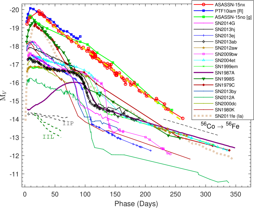
Figure 6: The absolute $V$-band light curve of ASASSN-15nx as compared to other Type II SNe and the Type Ia SN 2011fe. The exponential decline of a light curve following the radioactive decay law for ⁵⁶Co$\rightarrow$⁵⁶Fe is shown with a black dashed line. A best fit straight line (yellow dashed) is shown on top of ASASSN-15nx light curve to emphasize the linearity of decline. On the bottom left side, pairs of dashed lines in each gray and green colors represent the slope range for the Type II-P and II-L SNe templates as given by Faran et al. (2014). The adopted explosion time in JD-2400000, distance in Mpc, $E(B-V)$ in mag and the reference for observed V-band magnitude, respectively, are : SN 1979C – 43970.5, 16.0, 0.31; Barbon et al. (1982b); de Vaucouleurs et al. (1981); SN 1980K – 44540.5, 5.5, 0.30; Barbon et al. (1982a), NED database; SN 1987A – 46849.8, 0.05, 0.16; Hamuy & Suntzeff (1990); SN 1999em – 51475.6, 11.7, 0.10; Leonard et al. (2002); Elmhamdi et al. (2003); SN 2000dc – 51762.4, 49.0, 0.07; Faran et al. (2014), NED database; SN 2004et – 53270.5, 5.4, 0.41; Sahu et al. (2006); SN 2009bw – 54916.5, 20.2, 0.31; Inserra et al. (2012); SN 2012A – 55933.5, 9.8, 0.04; Tomasella et al. (2013); SN 2012aw – 56002.6, 9.9, 0.07; Bose et al. (2013); SN 2013ab – 56340.0, 24.0, 0.04; Bose et al. (2015a); SN 2013by – 56404.0, 14.8, 0.19; Valenti et al. (2015); SN 2013ej – 56497.3, 9.6, 0.06; Bose et al. (2015b); SN 2013hj – 56637.0, 28.2, 0.10; Bose et al. (2016); SN 2014G – 56669.7, 24.4, 0.25; Bose et al. (2016); PTF10iam – 55342.7, 453.35, 0.19; Arcavi et al. (2016); SN 2011fe – 55797.2, 6.79, 0.023; Munari et al. (2013); ASASSN-15no – 57235.5,153.5, 0.045; Benetti et al. (2018).

The characteristic radioactive tail phase of normal SNe II ($\gtrsim 150$ days), powered by ⁵⁶Co to ⁵⁶Fe decay, has a decline slope of $\sim 0.98~{}\mbox{mag (100 d)${}^{-1}$}$ when the $\gamma$-ray photons are fully trapped. During this phase, most SNe II in Fig. 6 shows a decline rate consistent with almost full trapping of the $\gamma$ rays. The light curve of ASASSN-15nx is significantly steeper and it continued to decline with a constant slope after the early peak. In comparison, the tail of the light curve of the prototypical Type Ia SN 2011fe (Munari et al., 2013), which is also powered by ⁵⁶Co to ⁵⁶Fe radioactive decay, has a slope comparable to ASASSN-15nx. The substantially lower $\gamma$-ray optical depth in SNe Ia increases the fraction of escaping $\gamma$-ray photons and makes the light curve steeper than typical SNe II. The similarity in light curve shapes between SNe Ia and luminous SNe IIL such as SN1979C has been discussed before (Doggett & Branch, 1985; Wheeler et al., 1987; Young & Branch, 1989), pointing to the possibility that luminous SN IIL might also be powered by the decay of a large mount of ⁵⁶Ni like SNe Ia. We explore this possibility for ASASSN-15nx  in §4.2 and §7.1.

In Fig. 7 we present the extinction corrected $(B-V)_{0}$ and $(V-I)_{0}$ color evolution of ASASSN-15nx  as compared with several SNe IIP/L and the Type IIL/n SN 1998S. For ASASSN-15nx, the magnitudes are loosely interpolated to match corresponding photometric epochs for each pair of bands, and this also serves to reduce the random fluctuations from internal uncertainties in the photometry. For $t<50$d ASASSN-15nx continues to become redder, following a similar trend to other SNe II. But after +50d, ASASSN-15nx shows a very little change in color, with mean values $(B-V)_{0}=0.450\pm 0.016$ and $(V-I)_{0}=0.598\pm 0.009$ mags, in contrast typical SNe IIP/L continues to evolve to substantially redder colors. However, SN IIL/n SN 1998S shows a color evolution similar to ASASSN-15nx in terms of the mean colors and the absence of evolution after $\sim 60$ days.

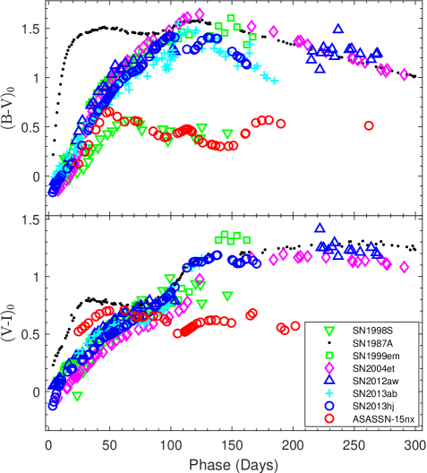
Figure 7: The color evolution of ASASSN-15nx as compared to the well-studied Type II SNe 1987A, 1999em, 2004et, 2012aw, 2013ab, 2014hj and also the type IIL/n SN 1998S. The references for the data are same as in Fig. 6.

We fit blackbody models to the extinction corrected B-, V- and I-band magnitudes. Fig. 8 shows the resulting evolution of the effective temperature and radius. Initially the radius increases until $+50$d, where the photospheric phase ends and the ejecta becomes optically thin. During this phase the temperature shows a steady decline as the ejecta cools down with expansion. The best-fit effective temperature then starts to rise until $\sim 135$d before again beginning a slow decline. This blackbody temperature evolution is unlike that of normal SNe, where we usually simply see monotonic declines (e.g., Bose et al., 2013, 2015a).

Figure 8: The temporal evolution of the blackbody temperature (blue, left scale) and radius (red, right scale) of ASASSN-15nx.

Figure 9: The UBVRI pseudo-bolometric light-curve of ASASSN-15nx as compared to other well-studied SNe. Light curves including UV contributions are also shown for SNe 2012aw, 2013ab and 2014G (labeled as UVO). The adopted distances, reddenings and explosion times are the same as in Fig. 6. The slope of a light curve powered by the radioactive decay of ⁵⁶Co$\rightarrow$⁵⁶Fe is shown with the dashed line.

4.2 Bolometric light curve and ⁵⁶Ni mass

In Fig. 9 we compare the pseudo-bolometric ($3335-8750$ Å) light curves of ASASSN-15nx with a sample of well-studied SNe II. The pseudo-bolometric luminosities for all SNe in the sample are constructed following the method described in Bose et al. (2013). The light curve decline rate for ASASSN-15nx is $1.05$ dex $(100\rm~{}d)^{-1}$, which is $\sim 3$ times faster than that expected for a light curve powered by the radioactive decay of ⁵⁶Co to ⁵⁶Fe.

Next we modeled the blackbody bolometric luminosity using a pure radioactive $\mbox{${}^{56}$Ni}\rightarrow\mbox{${}^{56}$Co}\rightarrow\mbox{${}^{56}$Fe}$ decay model. The two free model parameters are the ⁵⁶Ni mass $M_{Ni}$ and the $\gamma$-ray trapping parameter $t_{0\gamma}$, which defines the evolution of the $\gamma$-ray optical depth as $\tau_{g}\sim t_{0\gamma}^{2}/t^{2}$. While all the positron kinetic energy from ⁵⁶Co decay is trapped, only $[1-{\rm exp}(-t_{0\gamma}^{2}/t^{2})]$ fraction of the $\gamma$-ray decay energy is trapped in the envelope (see the discussions of this approximation in, e.g., Clocchiatti & Wheeler, 1997; Chatzopoulos et al., 2012). As shown in the top panel of Fig. 10, we find a reasonable fit for $M_{Ni}=1.6\pm 0.2$M_⊙ and a $\gamma$-ray trapping factor $t_{0\gamma}=73\pm 7$ days. Although the overall light curve is matched well by the model, there are some noticeable deviations at both early ($<25$ days) and late ($\sim 200$ days) times. Even if the light curve is entirely powered by the radioactive decay, this simple model is not expected to fully capture the light-curve evolution at early phases when the ejecta is optically thick and diffusion is important. The deviation at late time might reflect inaccuracies either in the physical assumptions of the simple radioactive decay model or the blackbody model used in deriving the bolometric light curve.

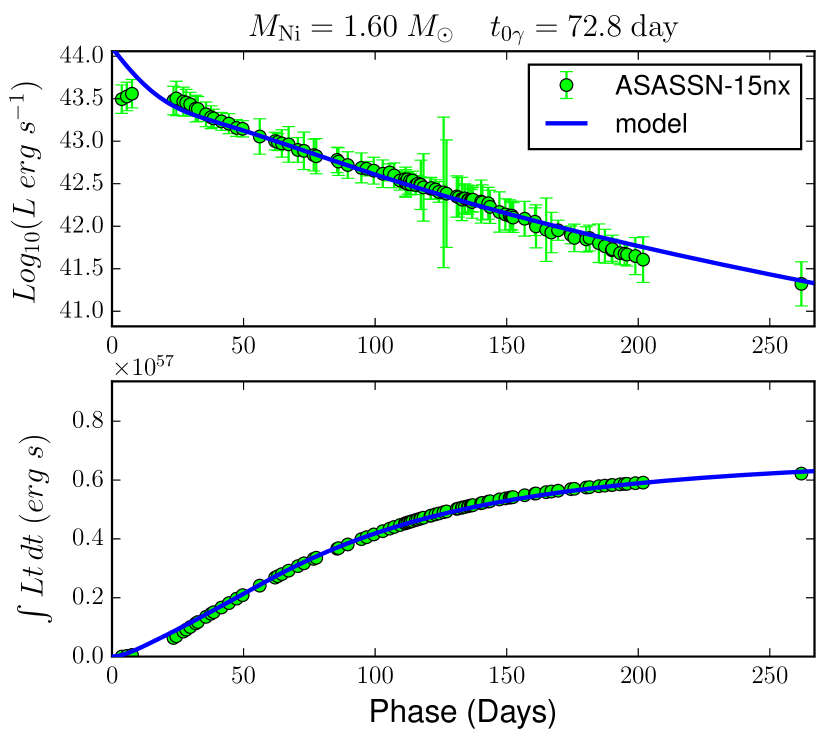
Figure 10: Radioactive decay models of the bolometric light curve (top panel) and the time-weighted integrated radiated energy (bottom panel) of ASASSN-15nx.

To gain more insight into the powering source, we also used the time-weighted integrated luminosity method to model the light curve (Katz et al., 2013; Nakar et al., 2016; Wygoda et al., 2017). The results are shown in the bottom panel of Fig. 10. By comparing time-weighted integrated luminosity with a radioactive decay model during the post-photospheric phase, we can verify the powering source of the entire light curve. Katz et al. (2013) showed that the time weighted integrated luminosity $(\int_{0}^{t}L(t^{\prime})t^{\prime}dt^{\prime})$ can also be used to put an additional constraint on the ⁵⁶Ni mass during the post-photospheric phase provided the light curve is solely powered by radioactive decay, as in SNe Ia. For this purpose early time estimates of the luminosity are required, so we extrapolated the temperature into the pre-peak phases and by scaling the SED to the V-band flux at fixed temperature. The blackbody luminosity is listed in Table 3. The uncertainty introduced by the extrapolation will eventually become smaller at larger values of $t$ due to the time weighting of the integral. The comparison of the integrated time weighted luminosity shows that the total energy budget of ASASSN-15nx is consistent with almost fully radioactive decay energy, which raises the possibility that it is the dominant powering source of the light curve.

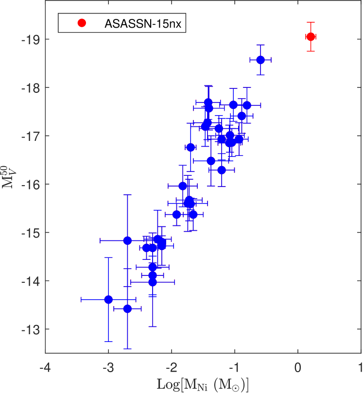
Figure 11: The absolute $V$ band magnitude at $t=50$ days as a function of the estimated ⁵⁶Ni mass for the SNe II sample, from Hamuy (2003) and Spiro et al. (2014). ASASSN-15nx, shown with filled red circle, lies on the extrapolation of the correlation to higher masses and luminosities.

In Fig. 11 we show the correlation between the ⁵⁶Ni mass and the V-band luminosity $M_{V}^{50}$ at $t=50$ days for the 34 Type II SNe from Hamuy (2003) and Spiro et al. (2014) along with ASASSN-15nx. As one would expect, ⁵⁶Ni mass increases with luminosity, however with considerable scatter in the correlation (see Pejcha & Prieto, 2015). ASASSN-15nx is consistent with an extrapolation of this correlation, while it clearly stands out at the higher extreme end of the luminosity distributions.

The black body model may not always be a good approximation, especially in the optical thin phases. We also constructed the bolometric light curve using bolometric corrections derived empirically from other well observed Type II SNe. The correction factor is calibrated as a function of broadband color. We adopt the bolometric correction from Bersten & Hamuy (2009) based on the $(B-V)$ color. Since B-band data is not available during the pre-peak phases, the $(B-V)$ color is linearly extrapolated from the color curve for $t<50$ days. By modeling this bolometric light curve we estimate $M_{Ni}=1.3\pm 0.2$M_⊙ and $t_{0\gamma}=71\pm 10$ days. This value of nickel mass is consistent within $\sim 20\%$ to that estimated with our earlier model, and the $\gamma$-ray trapping factor is also similar. We caution that the bolometric luminosities used in this method may also be inaccurate for an SN like ASASSN-15nx whose light curve, color and spectroscopic evolution is significantly different from generic SNe II.

5 Optical spectra

Figure 12: The rest-frame spectral evolution of ASASSN-15nx ordered by the age with respect to the explosion epoch JD 2457219.10. Prominent lines of hydrogen (H$\alpha$, H$\beta$), iron (Fe ii $\lambda\lambda$ 4924, 5018, 5169), sodium (Na i $\lambda$5890), calcium and oxygen are marked. Spectra with low SNR have been binned in wavelength to reduce the noise.

5.1 Key spectral features

The spectroscopic evolution of ASASSN-15nx fom $t=53$ to 262d is presented in Fig. 12. A striking feature is the H$\alpha$ emission profile, which has an unusual triangular shape in the earliest spectra at $t=53$d. We discuss the H$\alpha$ profile and its evolution further in §5.2 and §5.3. Forbidden [Ca ii] ($\lambda\lambda$7291, 7324) emission, which usually becomes visible not until the early nebular phase ($\gtrsim 120$ days), is visible throughout our observing campaign. The Ca ii multiplets ($\lambda\lambda$8498, 8542 and 8662) are not detected at $t=53.3$d, though the SNR in the relevant part of the spectrum is relatively low, while they are clearly visible at $t=87.4$d, which is typical of SNe IIP/L. O i emission near 7780Å is another prominent feature in the 53d spectra and is present throughout the spectral evolution. The strong O i emission feature appears unusually early for a Type II SN. Interestingly, the O i line has a doubly-peaked profile in the 53d spectra, which evolves into a singly-peaked profile by 96.7d and is no longer present in all subsequent spectra. The origin of the redder component of the double-peaked profile is not clear (as marked with a question mark in Fig. 12). The overall spectral appearance and the early presence of [Ca ii] and strong O i features in 53.0d make the spectrum appear much more evolved than typical SNe IIP/L at a similar phase. Another noticeable feature in all the spectra is the apparent continuum break near 5500Å. The continuum level on the bluer side is higher by about 25% than the red side (see further discussions in the context of synow modeling below and also in §7.2). The evolution of the prominent metallic lines of Fe ii ($\lambda\lambda$ 4924, 5018, 5169) and Na i D (5893 Å) is typical of SNe II.

Figure 13: synow model (blue) of the $t=53.0$ day spectrum of ASASSN-15nx (red). Observed fluxes are corrected for extinction. All ASASSN-15nx spectra show a break in the continuum near 5500Å, where the blue side has a higher flux level. To reproduce this feature, the model continuum is multiplied by the Gaussian convolved step function shown in the top panel.

We used synow (e.g. Fisher et al., 1997, 1999; Branch et al., 2002) to model the spectra and identify features. In order to mimic the continuum break, we multiply the model spectrum with a Gaussian convolved step function, whose amplitude and width are tuned to fit the observed spectrum. This modifier function is shown in the top panel of Fig. 13, where the bluer continuum beyond 5500Å is $\sim 25\%$ higher than the red with a 150Å width for the convolving Gaussian function.

The set of atomic species used to generate the synthetic spectrum are H i, He i, O i, Fe ii, Ti ii, Sc ii, Ca ii, Ba ii, Na i and Si ii. As noted above, ASASSN-15nx exhibits an unusual, triangularly-shaped H$\alpha$ emission with a weak absorption feature on the blue side is not consistent with a P-Cygni profile. The H$\beta$ profile is also unusually broad and extended, which synow could not reproduce with a single H$\beta$ component using any combination of expansion velocity and optical depth profile. So, the H$\alpha$ and H$\beta$ line region have been masked in the synthetic spectrum. Apart from the nebular-like emission features of Ca ii and O i, for which SYNOW is not applicable, many of the spectral features are reasonably well reproduced except for the Sc ii features at 4274Å and 4670Å.

In the synow model, the absorption feature near 6300Å which appears to form the absorption component of the P-Cygni profile associated with H$\alpha$, is reproduced by Si ii (6355Å). The Si ii velocity is same as the photospheric velocity ($\sim 3.3\mbox{$\times 10^{3}\rm{\,km\,s^{-1}}$}$) found for the other metal lines, affirming the line identification and suggesting that there is little or no absorption component associated with H$\alpha$.

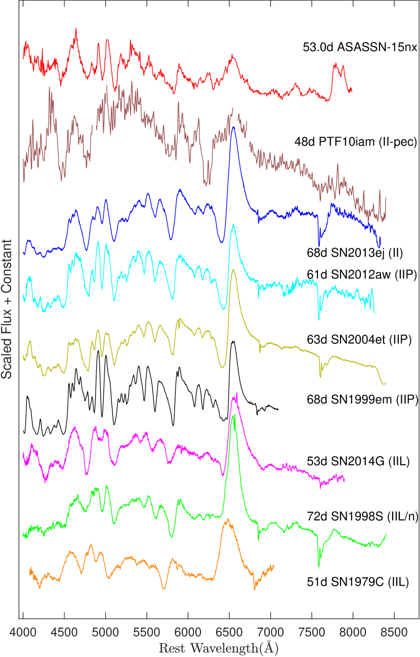
Figure 14: Comparison of the 53.0d spectrum of ASASSN-15nx to other Type II SNe 2013ej (Bose et al., 2015b), 2012aw (Bose et al., 2013), 2004et (Sahu et al., 2006), 1999em (Hamuy et al., 2001), 2014G Terreran et al. (2016), 1998S (Leonard et al., 2000; Fassia et al., 2001), PTF10iam (Arcavi et al., 2016) and 1979C (Branch et al., 1981) at similar age. All comparison spectra are corrected for extinction and redshift. For PTF10iam, the regions contaminated by host emission lines are masked.

Figure 15: Same as Fig. 14, but for the 121.0d ASASSN-15nx spectrum. The inset shows the H$\alpha$ region only, scaled to the peaks of the H$\alpha$ profiles.

Figure 16: Same as Fig. 14, but for a late phase (262.0d) spectrum of ASASSN-15nx.

5.2 Comparison of Spectra

We compare spectra of ASASSN-15nx to other Type II SNe at three different phases (53.0d, 121.0d, 262.0d) as shown in Figs. 14–16. Fig. 14 shows the comparisons of the 53.0d spectrum. Apart from the H$\alpha$ profile, the spectral features broadly resemble most of the other SNe II spectra in the comparison sample. The H$\alpha$ profile of ASASSN-15nx is significantly weaker and unusually triangular in shape as compared to other SNe II. For instance, normal SNe II at $t\approx 53$ days have a mean H$\alpha$ equivalent width of $\sim 157$Å (Gutiérrez et al., 2017), whereas for ASASSN-15nx we find a significantly lower value of $\sim 117$Å and it stays systematically weak throughout the evolution. P-Cygni H$\alpha$ profiles with an absorption component are common for most SNe II at this phase. But the absorption component of the H$\alpha$ profile appears to be non-existent for ASASSN-15nx, as in the synow model discussed above where the absorption feature blue-ward to the H$\alpha$ emission is identified as Si ii. The weakening of the H$\alpha$ absorption component has been generally seen for luminous and fast declining SNe IIL (see e.g., Gutiérrez et al., 2014) such as SN2014G, SN1998S and SN1979C shown in Fig. 14, and the absence of this absorption component in ASASSN-15nx is consistent with this trend. The H$\alpha$ profile for ASASSN-15nx also has an unusual triangular shaped peak compared to other known SNe II including SNe II-L. The doubly-peaked and exceptionally strong O i feature near 7700Å  is also not seen in any of the comparison spectra. The spectrum of PTF10iam, whose early-phase light curve closely resembles ASASSN-15nx (see Fig. 6) is also shown in Fig. 14. Apart from showing a weak and irregularly shaped H$\alpha$ profile, the spectrum of PTF10iam does not show any other similarities with ASASSN-15nx.

In Fig. 15 we compare the 121.0d spectrum with three other SNe II spectra at a similar age. The comparison spectra are specifically selected to show some form of irregularities or unusual shapes in their H$\alpha$ profiles. The ASASSN-15nx spectrum still has weaker H$\alpha$ emission. In the inset of the Fig. 15, we zoom into the H$\alpha$ line, scaling each spectra to the line peak. Unlike other SNe, the continuum of ASASSN-15nx on the blue side of H$\alpha$ has a higher flux level than on the red side. SNe 1999em and 2013ej both show asymmetric, possibly doubly-peaked components for H$\alpha$. Such profiles are often attributed to a bipolar distribution of ⁵⁶Ni in a spherically symmetric hydrogen envelope (Elmhamdi et al., 2003; Bose et al., 2015b). Similar asymmetric H$\alpha$ emission due to aspherical ⁵⁶Ni distribution has also been observed in SNe 1987A (Utrobin et al., 1995) and 2004dj (Chugai, 2006). The H$\alpha$ line profile of ASASSN-15nx appears to be even more complicated, and may also be composed of more than one component though not clearly separable. The wedge-shaped peak of ASASSN-15nx is similar to that of the Type II-L/n SN 1998S (Leonard et al., 2000), although the latter has a broader emission profile.

In Fig. 16 we compare the 262d spectrum with three other nebular-phase spectra of Type II SNe. ASASSN-15nx continues to have a weak and triangular H$\alpha$ profile. The nebular phase features, like forbidden [O i] near 6330Å and [Ca ii] near 7300Å, are significantly weaker than in the other SNe. The Na i D feature near 5900Å and the marginally visible Fe ii feature near 5000Å are comparable in strength with those of other SNe II.

Figure 17: Spectroscopic evolution in velocity domain corresponding to the H$\alpha$ and H$\beta$ rest wavelengths. The Fe ii multiplets are also in the H$\beta$ window.

5.3 Evolution of spectral features

In Fig. 17 we show the spectral regions centered on H$\alpha$ and H$\beta$ in velocity domain. The Fe ii multiplets ($\lambda\lambda$ 4924, 5018, 5169) do not show any significant evolution until the 233.9d spectrum. The Si ii (6355Å) absorption feature identified by synow in the 53d spectra is not detectable from 87d onwards. In the same wavelength range, the [O i] emission lines ($\lambda\lambda$ 6300, 6364; indicated in the figure) start to appear and become stronger at later times. For a typical Type II SN, the forbidden [O i] emission is seen only in nebular phase spectra at $t\sim 150$d. The H$\alpha$ profiles show a break or an abrupt change in slope on the blue wing of the line profile in all the spectra following 87d. This feature is marked as ‘A₁’ in Fig. 17 and in the inset of Fig. 15. The position of the A₁ feature is blue-shifted by $\sim 3.60\pm 0.25$$\times 10^{3}\rm{\,km\,s^{-1}}$ from the H$\alpha$ rest frame and remains almost unchanged after it appears at 87d. We also find a similar kink marked as ’A₂’ in the blue wing of the H$\beta$ profile. Interestingly, this feature also appeared from 87d onwards and is also blue-shifted by $\sim 3.60$$\times 10^{3}\rm{\,km\,s^{-1}}$ with respect to H$\beta$. The simultaneous appearance of A₁ and A₂ at consistent velocities suggests that the features must have common association with H i, rather than any possible blending with other spectral lines. However, the structural configuration of the H i materials needed to produce such an unusual feature is unclear.

The H$\alpha$ profile shows an atypical triangular shaped emission in the 53d spectra, and then developed a peculiar wedge shaped top at $\sim 87-123$ days. After this phase, the emission-top shows irregular and possibly multi-component emission features. The apparent absorption feature near 6400Å, which can be seen throughout the evolution maybe due to the Si ii absorption in the 53d spectra and the [O i] emission feature after 87d. This would imply that the H$\alpha$ line lacks the P-Cygni absorption component expected from a typical SN atmosphere. The H$\beta$ absorption is unusually broad and extended as compared to other SNe II (see Figs. 14 and 15), which synow model cannot fit with a single H i component. It is possible that multiple H$\beta$ absorption components are blended together to produce the broad feature. Such a scenario, with two H i components resulting in broader H$\alpha$ and H$\beta$ absorption profiles has been seen in SNe 2012aw (Bose et al., 2013) and 2013ej (Bose et al., 2015b). However, this explanation may not hold for ASASSN-15nx due to the missing H$\alpha$ absorption feature.

Figure 18: Velocity evolution of the H$\beta$, and Fe ii lines for ASASSN-15nx. The velocities are estimated from the blueshift of the apparent absorption minima. No attempt has been made to decouple any possible contamination from other lines or high-velocity features.

Figure 19: The photospheric velocity evolution ($v_{\rm ph}$) of ASASSN-15nx as compared with other well-studied Type II SNe. The $v_{\rm ph}$ is estimated by the Fe ii absorption trough velocities.

Figs 18 and 19 illustrate the spectroscopic velocity evolution of ASASSN-15nx. In Fig. 18 we show the H$\beta$ and Fe ii velocities using the blue-shifted absorption feature for each line. This includes no corrections for possible blended components. The H$\beta$ velocity evolution is puzzling, rising from 5.0$\times 10^{3}\rm{\,km\,s^{-1}}$ at 53d to $\sim 6.6$$\times 10^{3}\rm{\,km\,s^{-1}}$ at 87d and then continuing to increase. The peculiar H$\beta$ velocity evolution may indicate the presence of high-velocity components within the absorption profiles. An interaction of outer ejecta with CSM can produce such high-velocity components, which are expected to remain almost constant in velocity throughout the evolution (Chugai et al., 2007; Bose et al., 2015b; Gutiérrez et al., 2017). If the high-velocity component is strong enough, and the regular H$\beta$ component continues to become weaker, then the effective minima of the blended trough can show an increasing blueward shift, as we see in ASASSN-15nx. On the other hand, the Fe ii lines, which are generally regarded as good tracers of the photosphere, show almost no variation during the entire spectral evolution. In Fig. 19, the Fe ii line velocities of ASASSN-15nx are compared with other Type II SNe. Unlike the other SNe, the Fe ii velocity of ASASSN-15nx remains almost unchanged at $\sim 3.1$$\times 10^{3}\rm{\,km\,s^{-1}}$.

6 Summary of peculiarities

ASASSN-15nx exhibits a number of unusual features which can be summarized as follows.

1. The peak magnitude of $\sim-20$ lies in the luminosity “gap” between normal CCSNe and SLSNe.

2. It has a uniquely, long-lived, post-peak linear light curve decline with a steep slope of 2.5 mag (100 d)^-1 (i.e., an exponential decline in flux $\propto e^{-t/43{\rm d}}$) until the end. The perfectly linear light curve extended until end of observations at 262d. This is much longer than any known SNe IIP/L, which always show a change in light curve slope at around 100 days after maximum light, marking the transition to a ⁵⁶Co radioactive decay tail with a slope of 0.98 mag (100 d)^-1.

3. The broadband colors are almost constant and remain blue after 50 days. Equivalently, the blackbody temperature monotonically decreases until 50d as expected, reaching at $T\sim 5.8$kK. However, after this epoch we see an upward trend in the temperature reaching a value of $\sim 7.5$kK near 135d, before it again starts to decrease. Such an evolution has not been observed in any other SNe II.

4. The spectra of ASASSN-15nx shows unique, triangular H$\alpha$ emission profile throughout its evolution. The strength of the H$\alpha$ emission is weak compared to a typical SN II-P/L.

5. The H$\alpha$ profile shows no evidence for an associated P-Cygni absorption trough. The apparent absorption minima on the blue wing appears to be due to the presence of a Si ii feature at 53d, and then an [O i] feature at later times.

6. Nebular spectral features like O i (7774 Å), [Ca ii] ($\lambda\lambda$7291, 7324) and [O i] ($\lambda\lambda$6300, 6364) appeared earlier than in a typical SN II-P/L. For example, the [O i] features in typical SNe IIP appears after $\sim 150$ days, while in ASASSN-15nx they are detectable starting at 87d. Due to the presence of these features, the spectra of ASASSN-15nx appear more evolved than a typical SN II at similar age.

7. The O i (7774 Å) feature show a double peak emission at 53d. The unidentified redder component is much weaker at 87.4d and completely disappeared in later epoch.

8. The spectra all show an abrupt continuum break near 5500Å. The blue continuum is systematically brighter than the red (e.g., by $\sim 24$% at 53.0d).

9. There is a break in the blue wing of the both H$\alpha$ and H$\beta$ profiles (marked as ‘A₁’ and ‘A₂’ in Figs. 17 and 15), starting at 87d with a blueshifted velocity of $\sim 3.6$$\times 10^{3}\rm{\,km\,s^{-1}}$, indicating that both of these features have a common H i origin.

10. The H$\beta$ velocity shows an unusual increasing trend with time. The H$\beta$ absorption profile is also unusually broad and extended. This could not be reproduced by a single H i component in our synow models.

11. The Fe ii line velocities show no evolution, while in typical SNe, all line velocities are expected to decay with time.

7 Discussion

We are not aware of a theoretical model that can explain all the peculiarities of ASASSN-15nx. One important question is what powers this luminous SN II and how the long-lasting, “perfectly” linear light curve is produced, which are discussed in §7.1 and §7.2. In §7.3, we comment on the rate of ASASSN-15nx-like SNe.

7.1 High ⁵⁶Ni mass

One possible scenario for powering ASASSN-15nx is the synthesis of a large amount of radioactive ⁵⁶Ni. As discussed in §4.2, matching the high luminosity requires an exceptionally large amount of ⁵⁶Ni, $M_{Ni}=1.6\pm 0.2$ M_⊙. This is significantly higher than normal Type II SNe which have average $M_{Ni}$ of 0.05 M_⊙ and extend to at most $\sim 0.1-0.2$ M_⊙ (see e.g. Müller et al., 2017). For stripped envelope SNe, it can be as high as $0.6-0.7$ M_⊙ (e.g. for type Ic SN 2011bm; Valenti et al., 2012). The best-fit model also requires inefficient $\gamma$-ray trapping, with $t_{0\gamma}\approx 71$ days. For comparison, normal SNe IIP are consistent with complete trapping (i.e., $t_{0\gamma}\to\infty$), and for SNe Ia, $t_{0\gamma}\approx 40$ days (Wygoda et al., 2017). The value of $t_{0\gamma}$ for ASASSN-15nx implies that the envelope is inefficient at thermalizing the $\gamma$-rays. This is also consistent with the weak H$\alpha$ emission, because the hydrogen content in an SN ejecta is the dominant source of the $\gamma$-ray opacity.

The implied high ⁵⁶Ni mass and the short gamma-ray escape time of $t_{0}\sim 70~{}\rm day$ constrain the ejecta structure. The $\gamma$-rays must escape the region in the ejecta where the ⁵⁶Ni is concentrated allowing a constraint on the iron velocities. The $\gamma$-ray escape time of a homogeneous ball of iron with outer velocity $v_{\rm edge}$ and mass $M$ is

$$t_{0}=85{\rm d}~{}\left(\frac{M}{1.5~{}M_{\odot}}\right)^{0.5}\left(\frac{v_{\rm edge}}{5\times 10^{3}\mbox{$\rm{\,km\,s^{-1}}$}}\right)^{-1},$$ (1)

using an effective gamma-ray opacity of $\kappa_{\rm gamma}=0.025~{}\rm cm^{2}~{}g^{-1}$ (Swartz et al., 1995; Jeffery, 1999). This implies that the produced iron has to be distributed to velocities extending beyond $\sim 5\times 10^{3}\mbox{$\rm{\,km\,s^{-1}}$}$. Moreover, there is no room for significant additional mass at velocities $\lesssim 5\times 10^{3}\mbox{$\rm{\,km\,s^{-1}}$}$. Assuming that the hydrogen carries most of the energy it is useful to write the constraint for additional mass at higher velocities in terms of the total energy. The gamma-ray escape time from the center of a homogeneous ball of hydrogen with kinetic energy $E$ and mass $M$ is,

$$t_{0}=87{\rm d}\left(\frac{M}{2~{}M_{\odot}}\right)\left(\frac{E}{10^{51}\rm erg}\right)^{-1/2}.$$ (2)

For example, a Ni mass of $1.5\mbox{M${}_{\odot}$}$ extending to velocity $7\times 10^{3}\mbox{$\rm{\,km\,s^{-1}}$}$ embedded in a hydrogen ball of $1\mbox{M${}_{\odot}$}$ extending to $16\times 10^{3}\mbox{$\rm{\,km\,s^{-1}}$}$ would have a total gamma-ray escape time of 70 days and total energy of $2\times 10^{51}~{}\rm erg$, which are not inconceivable.

To get more insight into the envelope properties, we attempted simple semi-analytical model described by Arnett (1980) and Arnett & Fu (1989). The formulation and implementation of this model are discussed in Bose et al. (2015b) and references therein. This is a single component envelope model with radioactive ⁵⁶Ni confined at the center. This model is not fully applicable for ASASSN-15nx, as we observe no clear photospheric phase. However, by simply applying the model, we obtain an estimated envelope mass of $\sim 0.8-2.0$ M_⊙ with a thermal energy of $\approx 1.5\times 10^{51}$ erg. It is to be emphasized that these parameters are the upper limits, as with the increase of these values the model light curves show more sustained and prominent photospheric phases. For these parameters, the ejecta becomes optically transparent at $\sim 45$ days, which coincides with the break seen in B-band light curve, after which the light curve is solely powered by the $\mbox{${}^{56}$Ni}\rightarrow\mbox{${}^{56}$Co}\rightarrow\mbox{${}^{56}$Fe}$ decay chain. This low ejecta mass is consistent with the inefficient $\gamma$-ray trapping required for the radioactive decay model. Although we see the presence of H, O and Ca lines in the late spectra, as we see in typical SNe II with large ejecta masses, these lines are much weaker than typical SNe II (see Fig. 16), also suggestive of a low ejecta mass.

The large ⁵⁶Ni mass is consistent with the correlation between $M_{Ni}$ and V-band luminosity, as shown in Fig. 11. In this scenario, ASASSN-15nx might have produced a very large amount of radioactive ⁵⁶Ni with a significantly stripped envelope. However, it is not clear which mechanism could produce such a large mass of ⁵⁶Ni. One possible scenario is a thermonuclear explosion in a core-collapse supernovae (Kushnir & Katz, 2015; Kushnir, 2015b), which would produce a wide distribution of ⁵⁶Ni masses (Kushnir, 2015a). Pair instability explosions can also produce a large amount of ⁵⁶Ni with a wide range of luminosities, but they are also predicted to produce extended light curves (Kasen et al., 2011), different from that observed for ASASSN-15nx.

The possible production of a large amount of ⁵⁶Ni ($\sim 0.6\mbox{M${}_{\odot}$}$) in luminous and fast-declining SN II-L SN 1979C was raised by Doggett & Branch (1985); Wheeler et al. (1987); Young & Branch (1989). Later, Blinnikov & Bartunov (1993) showed that the high luminosity of SN 1979C in its photospheric phase could also be explained by the reprocessing of UV light into optical by an extended low mass hydrogen-helium envelope. However, despite the similarities in luminosity between ASASSN-15nx and SN 1979C in its early phases, there is a clear break in the light-curve slope of SN 1979C near 70 days indicating a change in the dominant energy source. As the ejecta becomes optically thin, the UV reprocessing ceases. While ASASSN-15nx does not show such a break, making it challenging to explain the prolonged, “perfectly” linear light curve of ASASSN-15nx solely with reprocessing of UV energy.

Another factor that may affect the ⁵⁶Ni  mass estimate is the asymmetry of the ejecta. Höflich et al. (1999) showed that for Type Ic-BL supernova 1998bw, an ejecta axis ratio of 2 may produce a 2 magnitudes of variation in peak luminosity between polar and equatorial directions. Polarimetric observations of SN 1998bw were also consistent with asymmetry in the ejecta of 1998bw. Polarimetry studies suggest that CCSNe, particularly those with relatively small envelope masses, may exhibit significant asymmetry in their ejecta (see e.g. Wang et al., 2001). If the ejecta of ASASSN-15nx  were highly asymmetric and viewed at a favorable angle, the actual amount of synthesized ⁵⁶Ni might be substantially reduced from the current estimate and shall produce its high peak luminosity. On the other hand, there is no strong evidence of asymmetry in the [O i] ($\lambda\lambda$6300, 6364) nebular lines as suggested by Taubenberger et al. (2009, 2013). However, quantitative modeling is needed to investigate whether an asymmetric model could explain the prolonged linear light-curve and spectroscopic features of ASASSN-15nx.

Synthesizing a large amount of radioactive ⁵⁶Ni normally should also lead to nebular-phase spectra rich with iron-group elements, as seen in Type Ia SNe, but this doesn’t appear to be the case with ASASSN-15nx. This could pose a serious challenge to the high ⁵⁶Ni mass scenario, and nebular-phase spectral modeling would be needed to examine it further.

7.2 CSM interaction

An alternative to the radioactive decay model is strong CSM interactions. In these models, the structure and distribution of the CSM can determine the shape of the light curves. As in SNe IIn (Schlegel, 1990), which are characterized by narrow emission lines (FWHM $\sim$ few hundreds of $\rm{\,km\,s^{-1}}$) in the spectra, strong interactions are thought to be responsible for powering their prolonged and often luminous light curves (e.g. Smith et al., 2008a; Rest et al., 2011). Sometimes ejecta-CSM interactions can lead to steeply declining light curves, as has been proposed for SN 2009jp (jet-CSM interaction; Smith et al., 2012b) and ASASSN-15no (Benetti et al., 2018). PTF10iam (Arcavi et al., 2016), which has early light curve features similar to ASASSN-15nx may also be explained by interaction .

The density profile of the CSM can be sculpted to produce the observed light curve of ASASSN-15nx. In ASASSN-15nx we do not see narrow or intermediate width emission lines from the expanding shock driving photo-ionization of the remaining CSM. It is possible to miss such emission lines if those were only present before our spectroscopic observations began at 53.0 days. However, this seems unlikely, as the continuous and linear decline of the light curve indicates a single dominant powering source throughout the evolution, which should produce similar narrow emission lines at later phases if they were present earlier. On the other hand, sometimes CSM signatures may also remain hidden if there is asymmetry or the CSM has a velocity of several thousands of $\rm{\,km\,s^{-1}}$.

Some of the spectral features in ASASSN-15nx can be attributed to indirect signatures of CSM interaction. synow model could not reproduce the broad and extended H$\beta$ absorption feature with a single, regular single H i component, and the steadily increasing H$\beta$ absorption velocity may indicate the presence of a blended high-velocity absorption component. In the case of CSM interactions relatively weaker than SNe IIn, the enhanced excitation of outer ejecta can produce high-velocity H i absorption features (e.g., SNe 1999em, 2004dj (Chugai et al., 2007), 2009bw (Inserra et al., 2012)), without producing narrow emission lines. In some other cases, the interaction signature can remain blended with regular H i P-Cygni profiles, e.g. SNe 2012aw (Bose et al., 2013), 2013ej (Bose et al., 2015b), where the two components can not be resolved individually, but resulting into broadening of H$\alpha$ and H$\beta$ absorption profiles. In ASASSN-15nx, as the strength of the regular component decays, the effective position of the blended absorption trough would shift to the blue. However, this would also require a similar high velocity absorption feature in the H$\alpha$ profile, which does not seem to be present, instead the entire absorption feature is missing in the SN. Another possibility is that that peculiar H$\alpha$ emission line profile might be composed of multiple components arising from CSM interactions.

The unusual rise in temperature from 50 to 135 days, which also coincided with the period of steady increase in the H$\beta$ velocity, might also be suggestive of CSM interaction. The increase in temperature could be due to the additional energy input from the ejecta interacting with CSM. The unusual break in the spectral continuum near 5500Å may be also explained with CSM interaction. Similar enhancements of the blue continuum have been seen in some strongly interacting SNe, such as SNe 2011hw (Smith et al., 2012a), 2006jc (Smith et al., 2008b) and 2005ip (Smith et al., 2009). The blue excess could be due to the blending of large number of broad and intermediate-width lines produced by the CSM interaction (Smith et al., 2012a; Chugai, 2009). In the case of SN 2005ip, the CSM lines were narrow enough to be seen forming the blue excess.

Another possible signature indicative of CSM interaction is the A₁ and A₂ pair of features, discussed in §5.3 (see Figs. 17, 15). The favorable aspect of this pair of features is that, both are located at the same blue-shifted velocity of $\sim 3.6$ $\times 10^{3}\rm{\,km\,s^{-1}}$, implying a common origin. This may indicate ejecta interacting with a clump or a shell of material is producing these H i features. However, it may be difficult to explain interaction powered light curve showing only these weak spectral signatures.

7.3 Rate for ASASSN-15nx like SNe

We can make two simple estimates of the rate of ASASSN-15nx-like transients, one based on a crude model of the ASAS-SN survey, and the other using a simple scaling based on the number of Type Ia SNe in ASAS-SN. Roughly speaking, ASAS-SN detects $V<17$ mag transients, which means that ASASSN-15nx could be detected to a comoving distance of $\sim 214$ Mpc, corresponding to a volume of $V=0.041$ Gpc³. The rate implied by finding one such event is

$$r=25\left({4\pi\over\Omega}\right)\left({\hbox{years}\over t_{eff}}\right)$$ (3)

where $\Omega\simeq 2\pi$ is the fraction of the sky being surveyed for SNe at any given time and $t_{eff}$ is the effective survey time. Roughly speaking, ASAS-SN has been running for 2.7 years, but finds only 70% of the $V<17$ mag SNe visible in its survey area, so $t_{eff}\simeq 1.8$ years. Combining these factors gives a rough rate estimate of $r\simeq 28$ Gpc^-3 year^-1. Alternatively, ASASSN-15nx is about one magnitude more luminous than a typical Type Ia SNe, implying an effective survey volume to find ASASSN-15nx-like events that is four times greater than for Type Ia SNe. In its first 2.7 years, ASAS-SN found a total of 449 Type Ia SNe, so the ASASSN-15nx-like event rate should be $r=r_{\rm Ia}/4/449$ correcting for the larger volume for detecting ASASSN-15nx ($4$) and the ratio of the numbers of the two events ($1:449$). The Type Ia SNe rate is $r_{\rm Ia}\simeq 3\times 10^{4}$ Gpc^-3 year^-1 (Li et al., 2011a), so $r\simeq 17$ Gpc^-3 year^-1, which is in good agreement with the first estimate. Thus, the rate of ASASSN-15nx-like transients is comparable to that for hydrogen-poor (Type I) SLSNe $r_{\rm SLSN-I}=91^{+76}_{-36}$ Gpc^-3 year^-1 derived by Prajs et al. (2017), raising the possibility that the previously identified luminosity “gap” between normal CCSNe and SLSNe might be due to observational selection effects.

Table 2: Summary of spectroscopic observations of ASASSN-15nx.

UT Date	JD	Phasea	Telescopeb
(yy/mm/dd.dd)	2457000+	(days)
2015-09-08.12	273.62	53.0	Coper
2015-09-08.38	273.88	53.3	Dup
2015-10-13.46	308.96	87.4	MOD
2015-10-22.00	318.50	96.7	Coper
2015-10-23.50	319.00	97.2	Bok
2015-11-05.09	331.59	109.4	NOT
2015-11-05.10	331.60	109.4	Coper
2015-11-16.99	343.49	121.0	Coper
2015-11-18.98	345.48	122.9	Coper
2015-11-19.30	345.80	123.2	Bok
2015-12-01.32	357.82	134.9	MMT
2015-12-02.97	359.47	136.5	Coper
2015-12-07.25	363.75	140.7	MOD
2015-12-17.96	374.46	151.1	Coper
2016-01-02.21	389.71	165.9	MOD
2016-01-02.29	389.79	166.0	Bok
2016-01-16.08	403.58	179.4	MagE
2016-03-12.09	459.59	233.9	IMAC
2016-04-10.01	488.51	262.0	IMAC

^a The phase is the number of rest frame days after the adopted explosion epoch JD 2457219.10

^b The telescope abbreviations are - Coper : Copernico telescope; Dup : Du Pont telescope; MOD: MODS spectrograph on LBT; Bok: Bok telescope; MMT: MMT Observatory; NOT: Nordic Optical Telescope; MagE: Echellette Spectrograph on Magellan Baade telescope; IMAC: IMACS spectrograph on Magellan Baade telescope.

Table 3: Black-body Bolometric luminosity.

Phasea	Luminosity	Phasea	Luminosity
(days)	($Log_{10}[L~{}erg~{}s^{-1}]$)	(days)	($Log_{10}[L~{}erg~{}s^{-1}]$)
3.72	43.49 $\pm$ 0.17	118.38	42.46 $\pm$ 0.40
5.65	43.53 $\pm$ 0.17	121.02	42.44 $\pm$ 0.13
7.59	43.56 $\pm$ 0.17	121.30	42.45 $\pm$ 0.13
23.37	43.48 $\pm$ 0.17	122.94	42.43 $\pm$ 0.11
24.44	43.50 $\pm$ 0.20	124.21	42.40 $\pm$ 0.12
27.10	43.47 $\pm$ 0.17	126.01	42.40 $\pm$ 0.89
28.20	43.45 $\pm$ 0.16	127.13	42.38 $\pm$ 0.63
29.72	43.44 $\pm$ 0.14	131.02	42.35 $\pm$ 0.24
31.82	43.38 $\pm$ 0.16	131.70	42.34 $\pm$ 0.23
32.63	43.38 $\pm$ 0.15	132.97	42.32 $\pm$ 0.25
35.71	43.32 $\pm$ 0.15	133.16	42.31 $\pm$ 0.17
37.65	43.28 $\pm$ 0.13	134.12	42.33 $\pm$ 0.17
38.63	43.27 $\pm$ 0.11	135.30	42.31 $\pm$ 0.17
41.61	43.23 $\pm$ 0.11	135.52	42.31 $\pm$ 0.14
44.44	43.21 $\pm$ 0.12	136.34	42.30 $\pm$ 0.13
47.34	43.16 $\pm$ 0.10	136.56	42.30 $\pm$ 0.13
49.66	43.15 $\pm$ 0.10	136.87	42.28 $\pm$ 0.19
56.14	43.06 $\pm$ 0.21	137.16	42.31 $\pm$ 0.14
61.98	43.00 $\pm$ 0.10	140.28	42.29 $\pm$ 0.25
63.02	42.99 $\pm$ 0.10	140.76	42.28 $\pm$ 0.21
64.56	42.97 $\pm$ 0.16	143.00	42.27 $\pm$ 0.19
67.12	42.96 $\pm$ 0.21	143.67	42.23 $\pm$ 0.19
70.64	42.90 $\pm$ 0.15	147.22	42.17 $\pm$ 0.24
72.94	42.89 $\pm$ 0.22	149.51	42.14 $\pm$ 0.18
76.66	42.84 $\pm$ 0.19	151.14	42.12 $\pm$ 0.19
77.63	42.82 $\pm$ 0.21	151.41	42.12 $\pm$ 0.16
85.57	42.78 $\pm$ 0.15	152.01	42.12 $\pm$ 0.17
86.10	42.76 $\pm$ 0.16	152.43	42.10 $\pm$ 0.17
89.58	42.72 $\pm$ 0.16	156.83	42.09 $\pm$ 0.20
94.77	42.69 $\pm$ 0.18	160.74	42.05 $\pm$ 0.16
96.74	42.68 $\pm$ 0.08	161.12	42.00 $\pm$ 0.25
99.47	42.65 $\pm$ 0.16	165.01	41.96 $\pm$ 0.37
102.90	42.62 $\pm$ 0.16	166.96	41.93 $\pm$ 0.24
105.52	42.63 $\pm$ 0.10	169.53	41.95 $\pm$ 0.12
107.23	42.60 $\pm$ 0.15	174.42	41.90 $\pm$ 0.10
109.48	42.54 $\pm$ 0.11	175.71	41.86 $\pm$ 0.16
111.34	42.55 $\pm$ 0.08	180.21	41.85 $\pm$ 0.15
111.57	42.51 $\pm$ 0.16	181.48	41.86 $\pm$ 0.15
111.60	42.52 $\pm$ 0.18	185.05	41.80 $\pm$ 0.23
112.30	42.55 $\pm$ 0.08	187.31	41.76 $\pm$ 0.20
112.54	42.50 $\pm$ 0.12	189.93	41.72 $\pm$ 0.13
113.25	42.53 $\pm$ 0.08	190.16	41.73 $\pm$ 0.16
113.52	42.49 $\pm$ 0.12	193.08	41.68 $\pm$ 0.14
114.24	42.54 $\pm$ 0.11	194.79	41.68 $\pm$ 0.13
115.46	42.48 $\pm$ 0.11	195.74	41.67 $\pm$ 0.14
116.19	42.50 $\pm$ 0.09	198.91	41.65 $\pm$ 0.22
117.14	42.49 $\pm$ 0.09	201.83	41.61 $\pm$ 0.27
117.39	42.49 $\pm$ 0.29	261.99	41.32 $\pm$ 0.26

The bolometric luminosity is calculated by fitting black-body on BVI bands photometric data. During pre-peak phases ($\leq 23.37$d), where only V-band data available, the blackbody temperature is extrapolated and luminosity is calculated after scaling the blackbody SED to match V-band data, also taking into account of the broadband filter response. At 261.99 days the fitting is done on $BVri$-bands data.

^aRest-frame days relative to the adopted explosion epoch JD 2457219.10.

References

- Anderson et al. (2014) Anderson, J. P., González-Gaitán, S., Hamuy, M., et al. 2014, ApJ, 786, 67
- Arcavi et al. (2012) Arcavi, I., Gal-Yam, A., Cenko, S. B., et al. 2012, ApJL, 756, L30
- Arcavi et al. (2016) Arcavi, I., Wolf, W. M., Howell, D. A., et al. 2016, ApJ, 819, 35
- Arnett (1980) Arnett, W. D. 1980, ApJ, 237, 541
- Arnett & Fu (1989) Arnett, W. D., & Fu, A. 1989, ApJ, 340, 396
- Astropy Collaboration et al. (2013) Astropy Collaboration, Robitaille, T. P., Tollerud, E. J., et al. 2013, A&A, 558, A33
- Barbon et al. (1979) Barbon, R., Ciatti, F., & Rosino, L. 1979, A&A, 72, 287
- Barbon et al. (1982a) —. 1982a, A&A, 116, 35
- Barbon et al. (1982b) Barbon, R., Ciatti, F., Rosino, L., Ortolani, S., & Rafanelli, P. 1982b, A&A, 116, 43
- Barnsley et al. (2012) Barnsley, R. M., Smith, R. J., & Steele, I. A. 2012, Astronomische Nachrichten, 333, 101
- Benetti et al. (2018) Benetti, S., Zampieri, L., Pastorello, A., et al. 2018, MNRAS, 476, 261
- Bersten & Hamuy (2009) Bersten, M. C., & Hamuy, M. 2009, ApJ, 701, 200
- Blinnikov & Bartunov (1993) Blinnikov, S. I., & Bartunov, O. S. 1993, A&A, 273, 106
- Bose et al. (2016) Bose, S., Kumar, B., Misra, K., et al. 2016, MNRAS, 455, 2712
- Bose et al. (2013) Bose, S., Kumar, B., Sutaria, F., et al. 2013, MNRAS, 433, 1871
- Bose et al. (2015a) Bose, S., Valenti, S., Misra, K., et al. 2015a, MNRAS, 450, 2373
- Bose et al. (2015b) Bose, S., Sutaria, F., Kumar, B., et al. 2015b, ApJ, 806, 160
- Bose et al. (2018) Bose, S., Dong, S., Pastorello, A., et al. 2018, ApJ, 853, 57
- Branch et al. (1981) Branch, D., Falk, S. W., Uomoto, A. K., et al. 1981, ApJ, 244, 780
- Branch et al. (2002) Branch, D., Benetti, S., Kasen, D., et al. 2002, ApJ, 566, 1005
- Brown et al. (2013) Brown, T. M., Baliber, N., Bianco, F. B., et al. 2013, PASP, 125, 1031
- Cardelli et al. (1989) Cardelli, J. A., Clayton, G. C., & Mathis, J. S. 1989, ApJ, 345, 245
- Chatzopoulos et al. (2012) Chatzopoulos, E., Wheeler, J. C., & Vinko, J. 2012, ApJ, 746, 121
- Chugai (2006) Chugai, N. N. 2006, Astronomy Letters, 32, 739
- Chugai (2009) —. 2009, MNRAS, 400, 866
- Chugai et al. (2007) Chugai, N. N., Chevalier, R. A., & Utrobin, V. P. 2007, ApJ, 662, 1136
- Clocchiatti & Wheeler (1997) Clocchiatti, A., & Wheeler, J. C. 1997, ApJ, 491, 375
- de Vaucouleurs et al. (1981) de Vaucouleurs, G., de Vaucouleurs, A., Buta, R., Ables, H. D., & Hewitt, A. V. 1981, PASP, 93, 36
- Doggett & Branch (1985) Doggett, J. B., & Branch, D. 1985, AJ, 90, 2303
- Dong et al. (2016) Dong, S., Shappee, B. J., Prieto, J. L., et al. 2016, Science, 351, 257
- Elias-Rosa et al. (2015) Elias-Rosa, N., Cappellaro, E., Benetti, S., et al. 2015, The Astronomer’s Telegram, 8016
- Elmhamdi et al. (2003) Elmhamdi, A., Danziger, I. J., Chugai, N., et al. 2003, MNRAS, 338, 939
- Faran et al. (2014) Faran, T., Poznanski, D., Filippenko, A. V., et al. 2014, MNRAS, 445, 554
- Fassia et al. (2001) Fassia, A., Meikle, W. P. S., Chugai, N., et al. 2001, MNRAS, 325, 907
- Filippenko (1997) Filippenko, A. V. 1997, ARA&A, 35, 309
- Fisher et al. (1999) Fisher, A., Branch, D., Hatano, K., & Baron, E. 1999, MNRAS, 304, 67
- Fisher et al. (1997) Fisher, A., Branch, D., Nugent, P., & Baron, E. 1997, ApJL, 481, L89
- Gal-Yam (2012) Gal-Yam, A. 2012, Science, 337, 927
- Gutiérrez et al. (2014) Gutiérrez, C. P., Anderson, J. P., Hamuy, M., et al. 2014, ApJL, 786, L15
- Gutiérrez et al. (2017) —. 2017, ApJ, 850, 89
- Hamuy (2003) Hamuy, M. 2003, ApJ, 582, 905
- Hamuy & Suntzeff (1990) Hamuy, M., & Suntzeff, N. B. 1990, AJ, 99, 1146
- Hamuy et al. (2001) Hamuy, M., Pinto, P. A., Maza, J., et al. 2001, ApJ, 558, 615
- Henden et al. (2016) Henden, A. A., Templeton, M., Terrell, D., et al. 2016, VizieR Online Data Catalog, 2336
- Höflich et al. (1999) Höflich, P., Wheeler, J. C., & Wang, L. 1999, ApJ, 521, 179
- Holoien et al. (2016a) Holoien, T. W.-S., Prieto, J. L., Pejcha, O., et al. 2016a, Acta Astron., 66, 219
- Holoien et al. (2016b) Holoien, T. W.-S., Kochanek, C. S., Prieto, J. L., et al. 2016b, MNRAS, 455, 2918
- Holoien et al. (2017a) Holoien, T. W.-S., Stanek, K. Z., Kochanek, C. S., et al. 2017a, MNRAS, 464, 2672
- Holoien et al. (2017b) Holoien, T. W.-S., Brown, J. S., Stanek, K. Z., et al. 2017b, MNRAS, 467, 1098
- Holoien et al. (2017c) —. 2017c, MNRAS, 471, 4966
- Inserra et al. (2012) Inserra, C., Turatto, M., Pastorello, A., et al. 2012, MNRAS, 422, 1122
- Jeffery (1999) Jeffery, D. J. 1999, ArXiv Astrophysics e-prints, astro-ph/9907015
- Kasen et al. (2011) Kasen, D., Woosley, S. E., & Heger, A. 2011, ApJ, 734, 102
- Katz et al. (2013) Katz, B., Kushnir, D., & Dong, S. 2013, ArXiv e-prints, arXiv:1301.6766
- Kiyota et al. (2015) Kiyota, S., Holoien, T. W.-S., Stanek, K. Z., et al. 2015, The Astronomer’s Telegram, 7895
- Kushnir (2015a) Kushnir, D. 2015a, ArXiv e-prints, arXiv:1506.02655
- Kushnir (2015b) —. 2015b, ArXiv e-prints, arXiv:1502.03111
- Kushnir & Katz (2015) Kushnir, D., & Katz, B. 2015, ApJ, 811, 97
- Leonard et al. (2000) Leonard, D. C., Filippenko, A. V., Barth, A. J., & Matheson, T. 2000, ApJ, 536, 239
- Leonard et al. (2002) Leonard, D. C., Filippenko, A. V., Gates, E. L., et al. 2002, PASP, 114, 35
- Li et al. (2011a) Li, W., Chornock, R., Leaman, J., et al. 2011a, MNRAS, 412, 1473
- Li et al. (2011b) Li, W., Leaman, J., Chornock, R., et al. 2011b, MNRAS, 412, 1441
- Lupton et al. (2005) Lupton, R. H., Jurić, M., Ivezić, Z., et al. 2005, in Bulletin of the American Astronomical Society, Vol. 37, American Astronomical Society Meeting Abstracts, 1384
- Müller et al. (2017) Müller, T., Prieto, J. L., Pejcha, O., & Clocchiatti, A. 2017, ApJ, 841, 127
- Munari et al. (2013) Munari, U., Henden, A., Belligoli, R., et al. 2013, New A, 20, 30
- Nakar et al. (2016) Nakar, E., Poznanski, D., & Katz, B. 2016, ApJ, 823, 127
- Pejcha & Prieto (2015) Pejcha, O., & Prieto, J. L. 2015, ApJ, 806, 225
- Piascik et al. (2014) Piascik, A. S., Steele, I. A., Bates, S. D., et al. 2014, in Proc. SPIE, Vol. 9147, Ground-based and Airborne Instrumentation for Astronomy V, 91478H
- Planck Collaboration et al. (2016) Planck Collaboration, Ade, P. A. R., Aghanim, N., et al. 2016, A&A, 594, A13
- Prajs et al. (2017) Prajs, S., Sullivan, M., Smith, M., et al. 2017, MNRAS, 464, 3568
- Quimby et al. (2007) Quimby, R. M., Aldering, G., Wheeler, J. C., et al. 2007, ApJL, 668, L99
- Rabinak & Waxman (2011) Rabinak, I., & Waxman, E. 2011, ApJ, 728, 63
- Rest et al. (2011) Rest, A., Foley, R. J., Gezari, S., et al. 2011, ApJ, 729, 88
- Sahu et al. (2006) Sahu, D. K., Anupama, G. C., Srividya, S., & Muneer, S. 2006, MNRAS, 372, 1315
- Schlafly & Finkbeiner (2011) Schlafly, E. F., & Finkbeiner, D. P. 2011, ApJ, 737, 103
- Schlegel (1990) Schlegel, E. M. 1990, MNRAS, 244, 269
- Shappee et al. (2014) Shappee, B. J., Prieto, J. L., Grupe, D., et al. 2014, ApJ, 788, 48
- Smith et al. (2008a) Smith, N., Chornock, R., Li, W., et al. 2008a, ApJ, 686, 467
- Smith et al. (2008b) Smith, N., Foley, R. J., & Filippenko, A. V. 2008b, ApJ, 680, 568
- Smith et al. (2012a) Smith, N., Mauerhan, J. C., Silverman, J. M., et al. 2012a, MNRAS, 426, 1905
- Smith et al. (2007) Smith, N., Li, W., Foley, R. J., et al. 2007, ApJ, 666, 1116
- Smith et al. (2009) Smith, N., Silverman, J. M., Chornock, R., et al. 2009, ApJ, 695, 1334
- Smith et al. (2012b) Smith, N., Cenko, S. B., Butler, N., et al. 2012b, MNRAS, 420, 1135
- Spiro et al. (2014) Spiro, S., Pastorello, A., Pumo, M. L., et al. 2014, MNRAS, 439, 2873
- Stetson (1987) Stetson, P. B. 1987, PASP, 99, 191
- Swartz et al. (1995) Swartz, D. A., Sutherland, P. G., & Harkness, R. P. 1995, ApJ, 446, 766
- Taubenberger et al. (2013) Taubenberger, S., Kromer, M., Pakmor, R., et al. 2013, ApJL, 775, L43
- Taubenberger et al. (2009) Taubenberger, S., Valenti, S., Benetti, S., et al. 2009, MNRAS, 397, 677
- Terreran et al. (2016) Terreran, G., Jerkstrand, A., Benetti, S., et al. 2016, MNRAS, 462, 137
- Tody (1993) Tody, D. 1993, in Astronomical Society of the Pacific Conference Series, Vol. 52, Astronomical Data Analysis Software and Systems II, ed. R. J. Hanisch, R. J. V. Brissenden, & J. Barnes, 173
- Tomasella et al. (2013) Tomasella, L., Cappellaro, E., Fraser, M., et al. 2013, MNRAS, 434, 1636
- Utrobin et al. (1995) Utrobin, V. P., Chugai, N. N., & Andronova, A. A. 1995, A&A, 295, 129
- Valenti et al. (2012) Valenti, S., Taubenberger, S., Pastorello, A., et al. 2012, ApJL, 749, L28
- Valenti et al. (2015) Valenti, S., Sand, D., Stritzinger, M., et al. 2015, MNRAS, 448, 2608
- Valenti et al. (2016) Valenti, S., Howell, D. A., Stritzinger, M. D., et al. 2016, MNRAS, 459, 3939
- Wang et al. (2001) Wang, L., Howell, D. A., Höflich, P., & Wheeler, J. C. 2001, ApJ, 550, 1030
- Wheeler et al. (1987) Wheeler, J. C., Harkness, R. P., & Cappellaro, E. 1987, in 13th Texas Symposium on Relativistic Astrophysics, ed. M. P. Ulmer, 402–412
- Wygoda et al. (2017) Wygoda, N., Elbaz, Y., & Katz, B. 2017, ArXiv e-prints, arXiv:1711.00969
- Young & Branch (1989) Young, T. R., & Branch, D. 1989, ApJL, 342, L79
Photometry of ASASSN-15nx.
\startlongtable| UT Date | JD | Phasea | B | V | R | I | g | r | i | Telescopeb |